Phase Fluctuations and Spectral Properties of Underdoped Cuprates

I Introduction.

It is now a well established experimental fact that the underdoped cuprate superconductors exhibit a “pseudogap” behavior above the superconducting critical temperature $T_{c}$, which is characterized by a vanishing superfluid density as obtained by transport measurements, but persistence of a gap in the quasiparticle excitation spectrum as measured by various spectroscopies[1]. Recent angle resolved photoemission (ARPES) [2, 3, 4, 5] and scanning tunneling spectroscopy (STS) [6, 7] experiments indicate that in the underdoped cuprates the gap evolves smoothly as the temperature is increased through $T_{c}$. Although the gap begins to fill in and the sharp quasiparticle peaks are lost above $T_{c}$, the position of the gap edge changes only slightly. This is in sharp contrast to the behavior of overdoped cuprates and conventional superconductors where the gap closes at $T=T_{c}$. It is further found that the gap increases as the doping concentration is reduced from its optimum value, while at the same time $T_{c}$ decreases. This results in highly anomalous ratios $2\Delta/k_{B}T_{c}$ which were reported to attain values of 12 or more in Bi₂Sr₂CaCu₂O_8+δ (BiSCCO), compared to the weak coupling BCS value of 3.54. ARPES results also indicate that the angular dependence of the gap function on the Fermi surface, which below $T_{c}$ follows the $\Delta_{\bf k}=\Delta_{d}\cos(2\theta)$ shape expected for a $d_{x^{2}-y^{2}}$ order parameter, develops extended gapless regions around the nodes above $T_{c}$ whose size increases with $T$. Although a number of important experimental issues remains to be settled, such as the temperature at which the pseudogap closes and its possible persistence in optimally and even overdoped cuprates suggested by the recent STS results[6], the basic picture of a superconducting quasiparticle gap persisting over a wide range of $T>T_{c}$ in underdoped materials is well established.

Many theoretical concepts, including spin fluctuations[8], condensation of preformed pairs[9], SO(5) symmetry[10] and spin-charge separation[11], have been invoked to explain the pseudogap behavior. In this paper we study the implications of a scenario put forward by Emery and Kivelson[12] who, following earlier work of Uemura and co-workers[13], proposed that the underdoped material above $T_{c}$ is in a state with a non-zero local amplitude of superconducting pairing, but is not truly superconducting due to thermal fluctuations in the phase of the order parameter. Within such a scenario the transition at $T_{c}$ is of the Kosterlitz-Thouless (KT) type, slightly rounded by the weak coupling between the copper-oxygen planes along the $c$-axis. In a strictly 2D system the KT transition is associated with proliferation of unbound vortex-antivortex pairs. Weak coupling between the planes leads to correlated motion between vortices in adjacent planes which form 3D vortex loops close to the critical temperature. The transition to the disordered phase is then characterized by the appearance of vortex loops with arbitrarily large radii[14].

In the present paper we study the spectral properties of a superconductor in the incoherent state above the phase disordering transition but below the mean field transition at which the local gap forms. We find that fluctuating currents arising from unbound vortex-antivortex pairs can contribute significantly to the ARPES and STS lineshape broadening in the low-energy region of the spectrum. By analyzing the experimental data we estimate the strength of these superconducting phase fluctuations and we deduce the vortex core energy.

We model the underdoped cuprate superconductor as a set of independent 2D superconducting layers, each undergoing a KT transition at a temperature $T_{\rm KT}$ which we identify with the superconducting critical temperature $T_{c}$. The weak interplane coupling, which we neglect, will affect the very long lengthscale physics (changing e.g. the universality class of the transition from KT to 3D XY), but should not affect the shorter lengthscale fluctuations which contribute to the electron spectral functions of interest here. The disordered state above $T_{\rm KT}$ can be thought of as a “soup” of fluctuating vortices with positive and negative topological charges and with total vorticity constrained to zero. Each of these vortices is surrounded by a circulating supercurrent which decays as $1/r$ with the distance from the core. Such supercurrents, within a semiclassical approximation, lead to a Doppler-shifted local quasiparticle excitation spectrum of the form[15, 16]

$$E_{\bf k}=E_{\bf k}^{0}+\hbar{\bf k}\cdot{\bf v}_{s}({\bf r}),$$ (1)

where ${\bf v}_{s}({\bf r})$ is the local superfluid velocity and $E_{\bf k}^{0}=\sqrt{\epsilon_{\bf k}^{2}+|\Delta_{\bf k}|^{2}}$ is the usual BCS spectrum. The change in the local excitation spectrum will affect the spectral properties of the superconductor in that the physically relevant spectral function must be averaged over the positions of fluctuating vortices.

This effect will be particularly pronounced in a $d$-wave superconductor since Eq. (1) implies formation of a region on the Fermi surface with $E_{\bf k}<0$ around a nodal point for arbitrarily small ${\bf v}_{s}({\bf r})$. Physically this corresponds to a region of gapless excitations on the Fermi surface which leads to a finite density of states (DOS) at the Fermi level. As first discussed by Volovik[17], a similar situation arises in the mixed state of a $d$-wave superconductor where the superflow around the field-induced vortices leads to the residual DOS proportional to $\sqrt{H}$. This unusual field dependence arises because the distance between vortices in the vortex lattice $d_{v}\sim H^{-1/2}$ and the average superfluid velocity projected onto a gap node direction is proportional to $d_{v}^{-1}$. At low $T$ and high field this implies a $\sim T\sqrt{H}$ contribution to the electronic specific heat which was indeed observed in the measurements on YBa₂Cu₃O_6.95 single crystals[18, 19]. In the present case, instead of a regular Abrikosov lattice of field-induced vortices, we consider a fluctuating plasma of thermally induced vortices and antivortices. The essential physics however remains the same.

II Theory: quasiparticle excitations coupled to phase fluctuations.

We shall be interested in how the supercurrents induced by phase fluctuations affect the spectral function of a superconductor, $A({\bf k},\omega)=-\pi^{-1}{\rm Im}{\cal G}({\bf k},\omega)$, which may be measured by ARPES and STS experiments. Here ${\cal G}({\bf k},\omega)$ is the diagonal part of the full superconducting Green’s function which solves the Gorkov equations for a $d$-wave superconductor, given in the Appendix. In the mean field approximation (neglecting, among other things, phase fluctuations) the diagonal Green’s function may be written as

$${\cal G}_{0}^{-1}({\bf k},\omega)=\omega-\epsilon_{\bf k}+i\Gamma_{1}-{\Delta_{\bf k}^{2}\over\omega+\epsilon_{\bf k}},$$ (2)

where, following [5], we have added to the usual mean-field solution a single particle scattering rate $\Gamma_{1}$. Note that this form of the scattering rate in ${\cal G}_{0}$ constitutes an non-trivial assumption. It is not pairbreaking, in the sense that it is ineffective at small $\omega$, $\epsilon_{\bf k}$; i.e. in the region $\omega<E_{\bf k}\sim\sqrt{\epsilon_{\bf k}^{2}+\Delta_{\bf k}^{2}}$. By contrast in a $d$-wave superconductor, a conventional scattering rate enters via the replacement $\omega\to\omega+i\Gamma$, leading to a broadening which is effective even at low $\omega$, $\epsilon_{\bf k}$. As shown by Norman et al.[5] the form given in Eq. (2) agrees with the ARPES data at $T<T_{c}$. We demonstrate below that it also agrees with STS.

At $T>T_{c}$ Norman et al.[5] showed that additional pairbreaking scattering is needed to account for the ARPES data, which they modeled phenomenologically by introducing another scattering rate $\Gamma_{0}\neq\Gamma_{1}$, making a replacement $\omega\to\omega+i\Gamma_{0}$ in the last term of Eq. (2). They suggested that $\Gamma_{0}$ could arise from exchange of pair fluctuations; we find, by explicitly evaluating the corresponding propagator[20], that this proposed mechanism does not account for the observed magnitude of $\Gamma_{0}$. This conclusion is supported by the results of Vilk and Tremblay[21].

We now discuss what we believe to be a more likely source of the pairbreaking scattering, namely supercurrents induced by phase fluctuations. In order to determine how ${\cal G}_{0}$ is changed in the presence of superflow it is useful to recall the origin of the energy shift in Eq.(1). This can be derived[15, 16] by assuming a state of uniform superflow with ${\bf v}_{s}=\hbar{\bf q}/m$ [22] induced by an order parameter of the form $e^{2i{\bf q}\cdot{\bf r}}\Delta_{\bf k}$. By solving the appropriate set of Bogoliubov-de Gennes equations and retaining only terms to linear order in ${\bf q}$, one finds that the energy is modified as indicated in (1) while the coherence factors are to the same order unchanged. This result is then semiclassically extended to non-uniform situations by assuming slow spatial variations of ${\bf v}_{s}({\bf r})$.

One can follow this exact procedure and solve the appropriate Gorkov equations for ${\cal G}_{\bf q}$ in the presence of superflow. One finds (see Appendix) the following intuitively plausible result which is exact for uniform flow up to terms linear in ${\bf q}$[23]:

$${\cal G}_{\bf q}({\bf k},\omega)={\cal G}_{0}({\bf k}-{\bf q},\omega-\eta),$$ (3)

where $\eta\equiv\hbar{\bf v}_{F}({\bf k})\cdot{\bf q}\simeq\hbar{\bf k}\cdot{\bf v}_{s}$. Here ${\bf v}_{F}({\bf k})=(\partial\epsilon_{\bf k}/\partial{\bf k})_{k=k_{F}}\simeq\hbar{\bf k}_{F}/m$ is the Fermi velocity and the last equality holds when the Fermi surface is approximately isotropic. In the following we shall assume that Eq. (3) can be applied locally when ${\bf v}_{s}({\bf r})$ varies slowly in space. Applying the above prescription to (2) one finds, again to the leading order in ${\bf q}$,

$${\cal G}_{\bf q}^{-1}({\bf k},\omega)=\omega-\epsilon_{\bf k}+i\Gamma_{1}-{(\Delta_{\bf k}-\zeta)^{2}\over\omega+\epsilon_{\bf k}-2\eta},$$ (4)

where $\zeta\equiv{\bf v}_{\Delta}({\bf k})\cdot{\bf q}$ with ${\bf v}_{\Delta}({\bf k})=(\partial\Delta_{\bf k}/\partial{\bf k})_{k=k_{F}}$. One can easily estimate $v_{\Delta}/v_{F}\sim(\xi_{0}k_{F})^{-1}\sim\Delta_{d}/\epsilon_{F}$ which is typically a small number in superconductor. We therefore expect that $\zeta\ll\eta$. A more detailed numerical analysis indeed shows that, as long as $\Delta_{d}/\epsilon_{F}$ is small compared to unity, the effect of $\zeta$ on the spectral lineshape is negligible compared to that of $\eta$, and will be dropped in the following.

A typical experimentally measured quantity, such as the ARPES or STS lineshape, will provide information on ${\cal G}_{\bf q}$ averaged over the phase fluctuations. Thus, we need to evaluate

$$\bar{\cal G}_{\bf q}({\bf k},\omega)=\int d\eta P(\eta){\cal G}_{\bf q}({\bf k},\omega),$$ (5)

where $P$ is the probability distribution of $\eta$ given by

$$P(\eta) = \langle\delta[\eta-\hbar{\bf k}\cdot{\bf v}_{s}({\bf r})]\rangle.$$ (6)

The angular brackets indicate thermodynamic averaging over the phase fluctuations in the ensemble specified by the 2D XY Hamiltonian[12]

$${{\cal H}_{XY}\over k_{B}T}={1\over 2}V\left(2m\over\hbar\right)^{2}\int{\bf v}_{s}^{2}({\bf r})d^{2}r,$$ (7)

where ${\bf v}_{s}({\bf r})$ is understood to contain both longitudinal (spin wave like) and transverse (vortex like) excitations. $V=V_{0}/k_{B}T$ is a dimensionless coupling constant and $V_{0}$ is related to the superfluid density $n_{s}$ by $V_{0}=\hbar^{2}n_{s}/4m$. In the nearest neighbor XY model, $k_{B}T_{KT}\simeq 0.9V_{0}$[12]; more generally $k_{B}T_{KT}=(\pi/2)V_{0}(T=T_{\rm KT})$[26]. Longitudinal phase fluctuations result in the spatial modulation of charge density and will be therefore suppressed by Coulomb interaction at long wavelengths. This interaction is not explicitly included in the XY Hamiltonian (7) but we return to it shortly.

The last term in Eq. (2) can be thought of as a superconducting self energy $\Sigma_{s}(\omega,{\bf k})$. Eqs. (4,5) then imply that the primary effect of the phase fluctuations is to smear the functional dependence of $\Sigma_{s}(\omega,{\bf k})$ on the energy variable, broadening the spectral lineshape. A more detailed analysis shows that $\eta$ acts primarily to fill in the gap, in a way similar to the inverse pair lifetime $\Gamma_{0}$ introduced by phenomenological considerations in Ref.[5]. $\Gamma_{1}$, on the other hand, does not affect the lineshape at low energies: notice that ${\cal G}_{0}({\bf k}_{F},\omega=0)=0$ for any $\Gamma_{1}$.

We now give a quantitative description of this broadening by explicitly evaluating $P(\eta)$ and the resulting lineshapes as a function of temperature. Making use of the identity $\delta(x)=(2\pi)^{-1}\int dse^{isx}$ Eq.(6) becomes

$$P(\eta)={1\over 2\pi}\int_{-\infty}^{\infty}dse^{is\eta}\left\langle e^{-is\hbar{\bf k}\cdot{\bf v}_{s}({\bf r})}\right\rangle.$$ (8)

To the leading order in cumulant expansion one can write $\langle e^{-is\hbar{\bf k}\cdot{\bf v}_{s}({\bf r})}\rangle=\exp[-{1\over 2}s^{2}\hbar^{2}k_{\alpha}k_{\beta}\langle v_{s}^{\alpha}v_{s}^{\beta}\rangle]$, where summation over repeated indices is implied and the spatial variable has been suppressed. This statement becomes exact when the transverse fluctuations can be represented by Gaussian degrees of freedom, as is done in the Debye-Hückel approximation employed below. The $s$-integral in (8) can now be explicitly carried out, yielding a Gaussian distribution

$$P(\eta)=(2\pi W)^{-1/2}e^{-\eta^{2}/2W},$$ (9)

with $W=\hbar^{2}k_{\alpha}k_{\beta}\langle v_{s}^{\alpha}v_{s}^{\beta}\rangle$. We have thus reduced the problem of finding the probability distribution $P$ to evaluation of a correlator $\langle v_{s}^{\alpha}v_{s}^{\beta}\rangle$. For a 2D system described by the Hamiltonian (7), this correlator has been considered by Halperin and Nelson [27]. They found, using a Debye-Hückel approximation valid for for $T$ well above $T_{KT}$,

$$\langle v_{s}^{\alpha}({\bf p})v_{s}^{\beta}(-{\bf p})\rangle={\hbar^{2}\over 2m^{2}V}\left[{p_{\alpha}p_{\beta}\over p^{2}}+{\delta_{\alpha\beta}-p_{\alpha}p_{\beta}/p^{2}\over 1+c_{3}\xi_{c}^{2}p^{2}/4\pi^{2}V}\right],$$ (10)

where ${\bf v}_{s}({\bf p})=\int d{\bf r}e^{-i{\bf p}\cdot{\bf r}}{\bf v}_{s}({\bf r})$. The first term in brackets comes from the longitudinal and the second from the transverse fluctuations. $c_{3}=(2E_{c}-\pi^{2}V_{0})/k_{B}T$ is a dimensionless quantity related to the density of vortices, $E_{c}$ is the vortex core energy and $\xi_{c}$ is the core cutoff.

Upon averaging over fluctuations the translational invariance is restored and we may evaluate the real space correlator at ${\bf r}=0$:

$$\langle v_{s}^{\alpha}(0)v_{s}^{\beta}(0)\rangle={1\over(2\pi)^{2}}\int d^{2}p\langle v_{s}^{\alpha}({\bf p})v_{s}^{\beta}(-{\bf p})\rangle.$$ (11)

Explicit integration finally yields, for $|{\bf k}|=k_{F}$,

$$W={\pi^{3}\Delta_{d}^{2}\over 8V}\left[1+{V\over c_{3}}\ln\left(1+{c_{3}\over V}\right)\right].$$ (12)

The short wavelength divergence in (11) has been cut off at $q_{c}=2\pi/\xi_{c}$ and we used the BCS relation $\xi_{c}=\hbar v_{F}/\pi\Delta_{d}$. The first term in brackets comes from longitudinal fluctuations and would be suppressed in realistic models in which the Coulomb interaction is important. The second term, $\alpha_{v}\equiv(V/c_{3})\ln(1+c_{3}/V)$, comes from transverse fluctuations due to vortices, and is always positive and smaller then 1 (this follows since $c_{3}>0$ is required by the stability of the system). To the extent that $E_{c}$ is independent of temperature the ratio $c_{3}/V$, and therefore $\alpha_{v}$, is $T$-independent. The primary $T$-dependence of $W$ therefore comes from $V$ in the prefactor. After expressing $V_{0}$ in terms of $T_{\rm KT}$, $W$ may be written as

$$W\simeq 3.48(1+\alpha_{v})(T/T_{KT})\Delta_{d}^{2}.$$ (13)

Eqs. (4), (5) and (9) describe the effect of classical phase fluctuations on the spectral function of a superconductor. From the knowledge of such a spectral function one can compute the respective ARPES and STS lineshapes, extract the parameter $W$, and compare it with the prediction given by Eq. (13). This will be done in the next section, but we first discuss the validity and some qualitative aspects of the results presented above.

Our results depend on three assumptions; that the electron Greens function may be calculated using semiclassical methods, that the phase fluctuations are quasi-static, and that there is a sufficiently wide KT temperature regime in which reasonably well defined vortex-antivortex plasma exists. The first of these assumptions applies when the coherence length is sufficiently larger than the inter electron spacing (i.e. $k_{F}\xi\gg 1$) and is the same assumption as underlies Volovik’s prediction[17] of a $\sim T\sqrt{H}$ dependence of the specific heat in the mixed state of a $d$-wave superconductor. As this behavior is observed in YB₂Cu₃O₇[18, 19], we believe that this assumption is well justified. The second assumption, of quasi-static phase fluctuations, has two parts. The transverse fluctuations come from vortices, so for them the essential assumption is that vortices move slowly compared to electrons. This is justified by Bardeen-Stephen results, which imply that vortex motion is overdamped and thus diffusive, and so surely slower than the ballistic motion of the electrons. For longitudinal fluctuations the situation is less clear. If the hypothesis of Emery and Kivelson, that they are classical (i.e. that at $q\sim\xi_{c}^{-1}$ we have $\omega_{q}\ll T$)[12] is accepted then Eq. (10) applies. However, as we shall see, the data contradict this. A more likely scenario is that Coulomb interaction pushes the longitudinal fluctuations up to the plasma frequency, in which case the coupling to electrons is very weak and one should simply remove the longitudinal fluctuations from the theory. We shall see that the data are consistent with this picture. If (for some as yet unknown reason) the longitudinal fluctuations are collective modes with a velocity of the order of the Fermi velocity, then our results do not apply. The final assumption, of a wide temperature regime between the mean-field and KT transitions, is the most difficult to justify, except on empirical grounds. This hypothesis was proposed in Ref.[12] and our results are consistent with it. The theoretical justification for a clean system must involve proximity to a Mott insulating phase, which suppresses the superfluid stiffness and hence $T_{KT}$, but does not suppress the pairing. A detailed theoretical treatment in two dimensions has not been given.

As mentioned above, $W$ given by Eq. (13) describes both longitudinal and transverse fluctuations of the phase and can be written accordingly as $W=W_{L}+W_{T}$, where

$$W_{L} \simeq 3.48(T/T_{KT})\Delta_{d}^{2},$$ (14)

$$W_{T} \simeq 3.48\alpha_{v}(T/T_{KT})\Delta_{d}^{2},.$$ (15)

The expression for $W_{T}$ is valid at temperatures well above $T_{\rm KT}$, where all pairs can be thought of as unbound and thermal energy dominates over the intervortex interaction[26]. Well below $T_{\rm KT}$, on the other hand, we expect $W_{T}=0$ since the vortices appear only in tightly bound pairs which contribute negligible supercurrent beyond the lengthscale set by the pair size and the pair density is exponentially small $\sim e^{-2E_{c}/k_{B}T}$. By numerically integrating the appropriate scaling relations[27] one could in fact obtain $W_{T}$ at all temperatures. However such level of detail is beyond the scope of this paper and we shall confine ourselves to the limiting cases stated above and note that $W_{T}$ has nonsingular monotonic behavior across $T_{\rm KT}$.

The expression (14) for $W_{L}$ is expected to be valid down to low temperatures, provided quantum fluctuations and the Coulomb interaction can be neglected. In a $d$-wave superconductor the temperature dependence of $W_{L}$ will be modified by the $T$-linear temperature dependence of the superfluid density[28] $n_{s}\sim\lambda^{-2}(T)$ which enters the definition of $V_{0}$ in the XY Hamiltonian (7). It is interesting to note that at temperatures below $T_{c}$, say at $T=T_{c}/2$, Eq. (14) implies $W_{L}\simeq\Delta_{d}^{2}$, i.e. large broadening of the spectral function by longitudinal fluctuations. Such a large broadening, comparable to the gap itself, would completely obliterate any signature of the gap in the excitation spectrum. Clearly, this is not observed experimentally[2, 3, 6]. As shown below and in Ref. [5], experimental data are consistent with $W=0$ below $T_{c}$. We must therefore conclude that longitudinal fluctuations are strongly suppressed by the Coulomb interaction as suggested in Ref.[29]. On the same grounds we may argue that the observed linear temperature dependence of the magnetic penetration depth[28] is not due to phase fluctuations, as suggested by some authors [30, 31], but due to thermally excited quasiparticles in the nodes of the $d$-wave gap[32]. Transverse fluctuations, on the other hand, result in no net charge displacement and are thus unaffected by Coulomb interaction.

III Comparison to experimental data

A Photoemission

As shown by Norman and co-workers[3], a particularly simple relationship exists between the spectral function of a superconductor and a symmetrized ARPES spectrum at the Fermi surface,

$$I_{S}(\omega)\propto{\bar{A}}({\bf k}_{F},\omega),$$ (16)

where $I_{S}(\omega)=I(\omega)+I(-\omega)$ and $I(\omega)$ is the measured ARPES lineshape. The advantage of this symmetrized representation is that the thermal broadening due to the Fermi functions is automatically subtracted out. The proportionality (16) is expected to hold for $|\omega|$ less then few tens of meV and remains valid in the presence of a symmetric energy resolution function. We first discuss qualitative features of our predicted lineshape and the experimental data, and then present results of a detailed fitting procedure.

The symmetrized experimental ARPES lineshapes for the 83K underdoped BiSCCO sample of Ref.[5] for the ${\bf k}={\bf k}_{F}$ vector along the $(0,0)\to(0,\pi)$ direction at selected temperatures are shown in Fig. 1(a). Below $T_{c}$ we wish to model these lineshapes by the spectral function corresponding to Eq. (2), which for ${\bf k}={\bf k}_{F}$, $\epsilon_{{\bf k}_{F}}=0$ becomes

$$I_{S}(\omega)\propto A_{0}({\bf k}_{F},\omega)={1\over\pi}{\Gamma_{1}\over(\omega-\Delta_{\bf k}^{2}/\omega)^{2}+\Gamma_{1}^{2}}.$$ (17)

As noted in [5], this functional form indeed describes the data below $T_{c}$ well, after it is convolved in $\omega$ with a Gaussian of width $\sigma=13.5$meV representing the estimated experimental resolution. Qualitatively, $\Delta_{\bf k}$ sets the position of the quasiparticle peaks and $\Gamma_{1}$ (together with $\sigma$) sets their width. Note that for $\Gamma_{1}=\sigma=0$ the above lineshape consists of two $\delta$-functions at $\omega=\pm\Delta_{\bf k}$. It is thus clear that fairly large values of $\Gamma_{1}$ in Eq. (17) are needed in order obtain quasiparticle peaks of the correct width. Even for large $\Gamma_{1}$ the theoretical lineshape $I(\omega)$ tends to zero for $|\omega|$ larger then several $\Delta_{\bf k}$, while the experimental lineshape saturates to a finite value. Understanding this large-$\omega$ background presents a challenge for any theory of ARPES in the cuprates and is beyond the scope of this paper. Here we focus on the low energy region of the spectrum where we may reasonably expect the present simple model to be valid.

For $\sigma\ll\Gamma_{1}$ one can easily estimate $I_{S}(0)\approx I_{0}(\Gamma_{1}\sigma^{2}/\Delta_{\bf k}^{4})$ and $I_{S}(\Delta_{\bf k})\approx I_{0}\Gamma_{1}^{-1}$. The peak to valley ratio

$$\kappa\equiv{I_{S}(\Delta_{\bf k})\over I_{S}(0)}\approx{\Delta_{\bf k}^{4}\over\Gamma_{1}^{2}\sigma^{2}}$$ (18)

is independent of the unknown prefactor $I_{0}$ and can be easily extracted from the raw data. Assuming fixed $\Delta_{\bf k}$ one can thus obtain reliable estimates of $\Gamma_{1}$ without performing detailed fits. In particular, application of Eq. (18) to the data in Fig. 1(a) implies that $\Gamma_{1}$ grows by about a factor of 6 between $T=14$K and 100K. The above analysis also implies that at low $\omega$ the lineshape depends crucially on the experimental resolution $\sigma$. For instance decreasing $\sigma$ by a factor of 2 the ratio $\kappa$ should grow by a factor of 4. Confirming this prediction experimentally would be a valuable test of the present model.

Above $T_{c}$ Eq. (17) no longer provides a good fit for the data. The reason for this is the persistence (up to $\sim 200$K) of a well defined edge-like feature around $\omega=\Delta_{\bf k}$ along with a pronounced increase in the low-$\omega$ density of states. This behavior cannot be modeled by further increasing $\Gamma_{1}$ since the values needed to fix $I(0)$ would rapidly smear the edge. Inclusion of the phase fluctuations, i.e. finite $W$ in the averaged spectral function (5), rectifies this problem. Analytically it is somewhat difficult to discuss the combined effect of $W$, $\Gamma_{1}$ and $\sigma$ on the lineshape. Qualitatively one can show that the primary effect of increasing $W$ is to “fill in” the gap. This is precisely what is needed to describe the ARPES data above $T_{c}$.

Fig. 1(a) shows our fit to the symmetrized ARPES lineshapes for the underdoped sample

FIG. 1.: a) Symmetrized ARPES lineshapes $I_{S}(\omega)$ at momentum near $(\pi,0)$ from Ref.[5] (thin line) and our fits to the spectral function (thick line) at selected temperatures. The dashed line illustrates fit with $W=0$. Region of the fit is $|\omega|<80$meV. b) Parameters of the fit as a function of $T$.

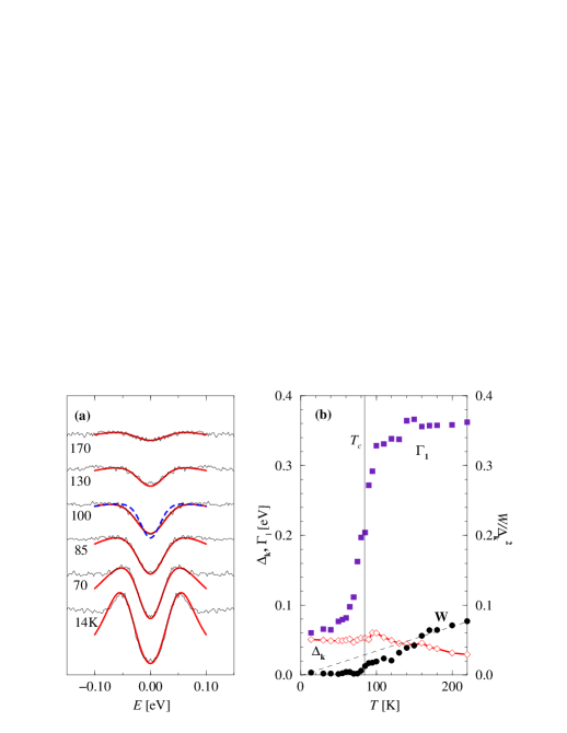
using a numerical computation of the full spectral function extracted from Eq. (5). Least square fits in which $\Delta_{\bf k}$, $\Gamma_{1}$ and $W$ were taken as free parameters, were performed after convolving the spectral function $\bar{A}({\bf k}_{F},\omega)$ with experimental resolution $\sigma=13.5$meV. In the low energy region $|\omega|\lesssim 80$meV, where the simple model Green’s function approach with $\omega$-independent scattering rate $\Gamma_{1}$ is expected to be valid, the fits are excellent for all temperatures. The extracted parameters are displayed in Fig. 1(b). Both $\Delta_{\bf k}$ and $\Gamma_{1}$ behave in the way expected for an underdoped cuprate: the gap is approximately constant across $T_{c}$ while the scattering rate rises sharply below $T_{c}$ and saturates at higher temperatures. In the present model the large increase in $\Gamma_{1}$ is required to wipe out the quasiparticle peaks. $W$ also behaves as anticipated from the above considerations. At low temperatures $W\simeq 0$ indicating that below $T_{c}$ the phase fluctuations are negligible; vortices appear only in tightly bound pairs and longitudinal fluctuations are suppressed by the Coulomb interaction. Above $T_{c}$ fluctuations become important (pairs unbind) and $W$ approaches the $T$-linear behavior consistent with (13). We stress here that a good fit to the data requires $W>0$ above $T_{c}$. This is illustrated by the dashed line in Fig. 1(a) which represents the fit to the 100K lineshape with $W=0$ and the gap value restricted to $\Delta_{\bf k}\lesssim\Delta_{\bf k}(T=0)$[33]. We note, however, that in this model much of the observed low-$\omega$ density arises from the large value of $\Gamma_{1}$ in combination with the instrumental resolution. It is possible (and is indeed suggested by the analysis of the STS data in the next section) that the large $\Gamma_{1}$ contribution is an artifact, arising from a combination of experimental resolution in the photoemission experiments and inadequacies of our theoretical model. We therefore regard the values of $W$ obtained here as underestimates.

From the slope of $W(T)$, assuming that transverse fluctuations are dominant, we estimate $\alpha_{v}\simeq 0.009$ implying the vortex core energy $E_{c}/V_{0}\simeq 360$. This value is much larger than the usual condensation energy in the vortex core $E_{c}\simeq 2V_{0}$ [16]. Within the Debye-Hückel approximation the vortex density can be estimated as $\rho_{v}=\xi_{c}^{-2}(\pi/c_{3})(1-\alpha_{v})\simeq\xi_{c}^{-2}(T/T_{\rm KT})(V/c_{3})$, for $\alpha_{v}\ll 1$ and $k_{B}T_{\rm KT}\simeq V_{0}$. This implies, for the parameters extracted from ARPES data, $\rho_{v}\simeq 4.3\times 10^{-3}\xi_{c}^{-2}(T/T_{\rm KT})$. It is remarkable that such a small density of vortices leads to significant broadening of the lineshape. We should also remark that for such a small density of vortices one may question the validity of Debye-Hückel approximation at temperatures in consideration. We emphasize, however, that only our interpretation of $W$ and in particular the estimates of $E_{c}$ and $\rho_{v}$ depend on the validity of this approximation. Our analysis of the lineshapes is quite general, since we treat $W$ as a free parameter of the model.

We have performed similar fits for an overdoped 82K BiSCCO sample of Ref.[5]. Our results are consistent with $\Delta_{\bf k}$ vanishing close to $T_{c}$ and, within statistical noise, $W=0$ at all temperatures. This indicates that phase fluctuations are unimportant in overdoped cuprates and the transition is essentially mean-field-like.

We now consider ARPES data at the Fermi crossing close to the gap node direction $(\pi,\pi)$. These indicate extended regions of gapless excitations above $T_{c}$ which grow in size with temperature[2, 3, 5]. This is not reproduced by the simple model we have considered so far. The reason is that adding the $\hbar{\bf v}_{s}\cdot{\bf k}$ term to the quasiparticle energy [cf. Eq.(3)] effectively depletes the local spectral function for ${\bf v}_{s}$ parallel to ${\bf k}$ but enhances it by equal amount for opposite ${\bf v}_{s}$. Upon averaging over all directions of ${\bf v}_{s}$ (for fixed ${\bf k}$) the net effect is to broaden the mean-field lineshapes as seen in Fig. 1(a). Phase fluctuations cause no net depletion of the spectral weight near the gap nodes.

In order to account for the ARPES data the form of $\Delta_{\bf k}$ must change. Since the supercurrent flowing around individual vortices is pair-breaking, it is in principle possible that it will alter the internal structure of the self-consistent gap function in addition to usual suppression of the order parameter in the core. A similar scenario has been proposed by Haas et al.[35] who considered the effect of non-magnetic impurities on a $d$-wave gap function. They found that it was possible to construct a gap function such that with increasing disorder nodes indeed expanded into finite gapless arcs. Intuitively this effect can be understood on the grounds that smaller gap near the nodes is more susceptible to the pair breaking. In the present case pair breaking is caused by supercurrents rather than impurities, but the physics remains the same.

In order to substantiate this idea we have solved the self-consistent gap equation for a $d$-wave superconductor in the presence of uniform superflow. We considered a model gap function of the form $\Delta_{\bf k}=\Delta_{d}\cos(2\theta)+\Delta^{\prime}_{d}\cos(6\theta)$ with the appropriately generalized pairing interaction[35]. We found that, for a system with $\Delta^{\prime}_{d}<0$ in the absence of superflow, a transition to $\Delta^{\prime}_{d}>0$ occurs when sufficiently strong supercurrent flows in the direction close to the nodal vector ${\bf k}_{n}$; i.e., when $|{\bf v}_{s}\cdot\hat{\bf k}_{n}|>b\Delta_{d}/\hbar k_{F}$, with $b\simeq 0.7$ a model dependent constant. The state with $\Delta^{\prime}_{d}>0$ exhibits extended gapless regions (cf. Fig. 2) while that with $\Delta^{\prime}_{d}<0$ only the usual point nodes. Extrapolating this behavior to the

FIG. 2.: Model gap function $\Delta(\theta)=\Delta_{d}\cos(2\theta)+\Delta^{\prime}_{d}\cos(6\theta)$ with $\tau\equiv\Delta^{\prime}_{d}/\Delta_{d}$ positive (extended nodes) and negative (point nodes). Inset illustrates the proposed real space electronic structure of the vortex in a $d$-wave superconductor.

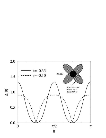
supercurrent flowing around the vortex we argue that a region of extended gapless excitations may form in the vicinity of the core. Such a region would have the shape of a four leaf clover (schematically depicted in the inset of Fig. 2) and a spatial extent of several $\xi_{c}$. A truly quantitative treatment of this effect is complicated because it involves self-consistently solving the $d$-wave vortex problem which is a highly non-trivial task[36]. We note, however, that recent STS data on vortices in BiSCCO[37], show a peculiar pseudogap behavior near the vortex core, which may be indicative of a formation of the gapless regions around a vortex proposed above.

Assuming that this picture is correct, it is clear that in the vortex-antivortex plasma above $T_{c}$, upon averaging over fluctuations, ARPES will detect a gap function strongly suppressed for ${\bf k}$ close to the nodes. Furthermore, with increasing temperature the volume fraction of gapless regions will grow (since the vortex density grows) leading to larger gapless areas on the Fermi surface in agreement with experimental observation.

B Tunneling

Tunneling conductance, the quantity measured by STS, is related to the spectral function of the superconductor by

$$g(E)=\int_{-\infty}^{\infty}d\omega f^{\prime}(\omega-E)\sum_{\bf k}|M_{\bf k}(\omega)|^{2}\bar{A}({\bf k},\omega),$$ (19)

where $f$ is the Fermi function and $M_{\bf k}(\omega)$ is the tunneling matrix element, usually approximated by a constant. Tunneling conductance reflects the spectral function averaged over the entire Brillouin zone and broadened in the energy variable by the Fermi function. Thus, unlike in the ARPES lineshape function $I_{S}(E)$, quasiparticle peaks in $g(E)$ will be broadened even in the absence of scattering and at $T=0$. For measurements performed on similar samples one would thus expect ARPES spectra to be much sharper than STS spectra, at any temperature. Fig. 3(a) displays $g(E)$ as measured by STS on 83K underdoped BiSSCO sample of Ref. [6]. Surprisingly, we observe that at lowest available temperatures STS line is in fact sharper than the ARPES line. As discussed in the previous section the broadening of the ARPES line comes exclusively from the scattering and experimental resolution. Therefore, inspection of the raw data suggests that the scattering rate $\Gamma_{1}^{\rm STS}$ will be much smaller than $\Gamma_{1}^{\rm ARPES}$. This conclusion is indeed borne out by the detailed fitting procedure carried out below. This is a rather surprising result which we discuss more fully in the next section.

As seen from Eq. (19), modeling of the tunneling conductance requires knowledge of the band structure away from the Fermi surface and is therefore somewhat more involved than that of ARPES. Nevertheless, we find that assuming a simple free electron dispersion with cylindrical Fermi surface and $\Delta_{\bf k}=\Delta_{d}\cos(2\theta)$, provides a reasonable fit for the data at low temperatures, provided that one compensates for the asymmetric background conductance and assumes $\theta$-dependent matrix element $M_{\bf k}(\omega)\propto|\cos(2\theta)|$. The latter assumption is motivated by band structure calculations[38] which indicate that tunneling between layers is dominated by the regions on the Fermi surface close to the $(0,\pi)$ points. As shown in Fig. 3(a), this $\theta$-dependence allows to

FIG. 3.: a) Fit to the STS data of Ref. [6] at selected temperatures. b) Parameters of the fit as a function of $T$. Above $T_{c}$ both $\Delta_{d}$ and $\Gamma_{1}$ are fixed to their values at 84K.

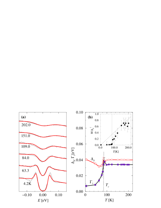
simultaneously account for the sharp quasiparticle peak and the wide gap in the STS line. Assuming $M_{\bf k}(\omega)$=const leads to broader peaks and sharper V-shaped gap structure, inconsistent with experimental data. We further remark that our simple model does not (and is not expected to) explain the pronounced dip feature appearing in the spectrum at higher energies, whose origin is at present unknown. Over the range $T<T_{c}$ $\Gamma_{1}^{\rm STS}$ has similar qualitative behavior as $\Gamma_{1}^{\rm ARPES}$ [compare Figs. 1(b) and 3(b)], but remains about one order of magnitude smaller. We have attempted to reconcile the two sets of data by considering a more realistic band structure and $\theta$-dependent scattering rate in Eq.(19). However, even under the most favorable conditions $\Gamma_{1}^{\rm STS}$ remains factor of 5-6 smaller than $\Gamma_{1}^{\rm ARPES}$.

Above $T_{c}$ the STS line does not have enough features to permit a meaningful three parameter fit. In particular the sharp gap edge completely disappears above 100K which leads to ambiguity in defining $\Delta_{d}$ from the data. Based on our previous finding (from the ARPES data) that both $\Delta_{d}$ and $\Gamma_{1}$ exhibit only weak $T$-dependence above $T_{c}$, we fix these two parameters at their respective values at 84K (40meV and 34meV) and extract the temperature dependence of $W$. This appears to us as a reasonable procedure which we further check by performing two-parameter fits with $\Delta_{d}$ held constant or slowly decreasing with temperature as implied by Fig. 1(b). $W$ is shown in the inset to Fig. 3(b). Its qualitative behavior is similar to that of $W^{\rm ARPES}$ but the amplitude is roughly factor of 10 larger. The difference is caused in part by the much smaller value of $\Gamma_{1}$ discussed above. Part of the discrepancy between $W^{\rm ARPES}$ and $W^{\rm STS}$ can presumably be attributed to differences in material and experimental uncertainties, as well as the failure of our fit to account for the temperature variation of $\Gamma_{1}$, which according to Fig. 1(b) grows by another factor of 2 between 80K and 200K. Nevertheless, after accounting for these factors, considerable discrepancy remains in place which is not understood at present. We estimate $\alpha_{v}\simeq 0.097$ which implies the vortex core energy $E_{c}\simeq 22V_{0}$ and vortex density $\rho_{v}\simeq 8.7\times 10^{-2}\xi_{c}^{-2}(T/T_{\rm KT})$. The value of $E_{c}/V_{0}$ is still large compared to the conventional estimate of the condensation energy in the core $E_{c}\simeq 2V_{0}$ [16], but is consistent with large core energy $E_{c}\simeq 26V_{0}$ deduced from lower critical field measurements of YBa₂Cu₃O_6.95 at $T=0$[34]. We note that $E_{c}$ is a cutoff-dependent quantity and therefore the precise numerical value quoted here should be accepted with that in mind. It is also possible that the large value of the ratio $E_{c}/V_{0}$ is due to an unusually small $V_{0}$ rather than unusually large $E_{c}$. Indeed, the vortex core energy is typically of the order of Fermi energy. Estimate of $V_{0}$ given in Ref. [29], $5$meV$<V_{0}<10$meV, implies $E_{c}\sim 0.1-0.2$eV, in reasonable agreement with many theories of underdoped cuprates which suggest a Fermi energy of the order of the exchange constant $J\sim 0.15$eV.

IV Discussion

The qualitative behavior of ARPES and STS lineshapes in underdoped BiSCCO clearly establishes the existence of a scattering mechanism which becomes operative at $T>T_{c}$ and which acts primarily to fill in the gap at low energies. We have shown that transverse phase fluctuations associated with proliferation of unbound vortex-antivortex pairs in the system provide a reasonable explanation for this scattering. Our analysis also indicates that longitudinal (spin wave) fluctuations are almost completely suppressed, above and below $T_{c}$. It has been proposed [30, 31] that in high-$T_{c}$ materials, longitudinal phase fluctuations governed by the XY Hamiltonian (7) are important in that they significantly contribute to the observed temperature dependence of the magnetic penetration depth[28]. We have calculated the broadening of the spectral function which would be caused by these fluctuations, and found it to be much greater than the experimental data would permit. We therefore conclude that longitudinal fluctuations are suppressed, perhaps by the Coulomb interaction as suggested in Ref. [29].

Quantitatively there exists considerable discrepancy between the parameters describing the ARPES and STS lineshapes, in particular the single particle scattering rate $\Gamma_{1}$ and phase fluctuation broadening $W$. Since the discrepancy is apparent at low temperatures and in overdoped cuprates we are led to believe that the problem lies primarily in our lack of detailed understanding of the lineshapes rather than the physics of phase fluctuations above $T_{c}$. The most disturbing is almost an order of magnitude difference between $\Gamma_{1}^{\rm ARPES}$ and $\Gamma_{1}^{\rm STS}$ found below $T_{c}$, which is implied directly by the raw data. In view of the fact that both measurements pertain to underdoped BiSCCO crystals with similar critical temperatures, it appears unreasonable to attribute such a large discrepancy to the material differences. We speculate that the large scattering rate needed to fit the ARPES data is an artifact related to our incomplete understanding of the photoemission process in the superconductor which is theoretically not completely understood even in simple metals[25]. Tunneling spectroscopy, on the other hand, is a technique well established in superconductors. We therefore surmise that parameters obtained from STS more directly reflect the underlying physics. Indeed $\Gamma_{1}^{\rm STS}\simeq 8$meV at 4.2K is comparable to the scattering rates deduced from transport measurements[39, 40] on underdoped cuprates, and $E_{c}^{\rm STS}\simeq 22V_{0}$, although large for a conventional superconductor, is perhaps not unreasonable in cuprates[34]. Consequently, ARPES lineshapes appear to reflect significant extrinsic broadening of unknown origin. The puzzling aspect of this interpretation is that the additional physics in the ARPES spectra enters as a multiplicative rather than additive factor to the apparent scattering rate; cf. $\Gamma_{1}^{\rm ARPES}\simeq 8\Gamma_{1}^{\rm STS}$ over the entire temperature range below $T_{c}$, in which $\Gamma_{1}$ changes by a factor of 6. It is also possible that in the cuprates the $c$-axis tunneling matrix element $M_{\bf k}(\omega)$ introduced in Eq. (19) is itself anomalous. Improving the energy resolution $\sigma$ of ARPES could shed some light on this issue. As noted below Eq. (18) the ARPES lineshapes are strongly affected by experimental resolution at small $\omega$. If the model Green’s function (2) is correct, a factor of two improvement in $\sigma$ should lead to considerable decrease in the measured intensity at $\omega=0$ but almost no change in the width or height of the quasiparticle peaks at $|\omega|=\Delta_{\bf k}$.

Finally we note that sizable transverse phase fluctuations implied by this work will also affect other properties of the underdoped systems, such as the electronic specific heat, fluctuation diamagnetism and transport. Vortices existing above $T_{c}$ should also generate local magnetic fields which are zero on average but have a non vanishing variance. If such fields could be detected, e.g. by muon spin rotation experiment, this would constitute a direct evidence for the phase fluctuation model of the pseudogap phase.

Gorkov equations in the presence of superflow

Real-space Gorkov equations[41] generalized to anisotropic superconductors read

$$(\omega-\hat{\cal H}_{e}){\cal G}({\bf r}_{1},{\bf r}_{2};\omega)+\hat{\Delta}{\cal F}^{+}({\bf r}_{1},{\bf r}_{2};\omega) = \delta({\bf r}_{1}-{\bf r}_{2}),$$ (20)

$$(\omega+\hat{\cal H}_{e}^{*}){\cal F}^{+}({\bf r}_{1},{\bf r}_{2};\omega)+\hat{\Delta}^{*}{\cal G}({\bf r}_{1},{\bf r}_{2};\omega) = 0.$$ (21)

Here $\hat{\cal H}_{e}=[i\nabla-(e/c){\bf A}]^{2}/2m-\epsilon_{F}$ is the single electron Hamiltonian and $\hat{\Delta}$ is the gap operator for spin singlet superconductivity defined as

$$\hat{\Delta}{\cal F}^{+}({\bf r}_{1},{\bf r}_{2};\omega)=\int d^{2}r^{\prime}\Delta({\bf r}_{1},{\bf r}^{\prime}){\cal F}^{+}({\bf r}^{\prime},{\bf r}_{2};\omega).$$ (23)

$\Delta({\bf r}_{1},{\bf r}_{2})$ is the gap function which is in general a nontrivial function of both electron coordinates in the anisotropic superconductor. We are interested in the state of uniform superflow induced by the gap function of the form

$$\Delta({\bf r}_{1},{\bf r}_{2})=\Delta_{0}({\bf r}_{1}-{\bf r}_{2})e^{i{\bf q}\cdot({\bf r}_{1}+{\bf r}_{2})}$$ (24)

and ${\bf A}=0$. The easiest way to solve (LABEL:gor1) for ${\cal G}$ is to perform a gauge transformation to the gauge where the order parameter is real and independent of the center of mass coordinate ${\bf R}=({\bf r}_{1}+{\bf r}_{2})/2$:

$$\Delta({\bf r}_{1},{\bf r}_{2}) \to \Delta({\bf r}_{1},{\bf r}_{2})e^{-i{\bf q}\cdot({\bf r}_{1}+{\bf r}_{2})},$$ (25)

$${\bf A} \to {\bf A}-{c\over e}{\bf q},$$ (26)

$${\cal G}({\bf r}_{1},{\bf r}_{2};\omega) \to {\cal G}({\bf r}_{1},{\bf r}_{2};\omega)e^{-i{\bf q}\cdot({\bf r}_{1}-{\bf r}_{2})},$$ (27)

$${\cal F}^{+}({\bf r}_{1},{\bf r}_{2};\omega) \to {\cal F}^{+}({\bf r}_{1},{\bf r}_{2};\omega)e^{i{\bf q}\cdot({\bf r}_{1}+{\bf r}_{2})}.$$ (28)

It is easy to verify that under such transformation Eqs. (LABEL:gor1) remain invariant[41]. In the new gauge Gorkov equations are manifestly translationaly invariant, i.e. independ of ${\bf R}$. Fourier transforming in the relative coordinate ${\bf r}={\bf r}_{1}-{\bf r}_{2}$ leads to algebraic equations for ${\cal G}$ and ${\cal F}^{+}$ of the form

$$(\omega-\epsilon_{{\bf k}-{\bf q}}){\cal G}({\bf k},\omega)+\Delta_{\bf k}{\cal F}^{+}({\bf k},\omega) = 1$$ (29)

$$(\omega+\epsilon_{{\bf k}+{\bf q}}){\cal F}^{+}({\bf k},\omega)+\Delta_{\bf k}{\cal G}({\bf k},\omega) = 0,$$ (30)

where $\epsilon_{\bf k}={\bf k}^{2}/2m-\epsilon_{F}$. The solution for ${\cal G}$ is

$${\cal G}_{\bf q}^{-1}({\bf k},\omega)=\omega-\epsilon_{{\bf k}+{\bf q}}-{\Delta_{\bf k}^{2}\over\omega+\epsilon_{{\bf k}-{\bf q}}}.$$ (31)

Expanding $\epsilon_{{\bf k}\pm{\bf q}}$ to leading order in ${\bf q}$ we obtain

$${\cal G}_{\bf q}^{-1}({\bf k},\omega) = (\omega-\eta)-\epsilon_{{\bf k}}-{\Delta_{\bf k}^{2}\over(\omega-\eta)+\epsilon_{{\bf k}}}$$ (32)

$$= {\cal G}_{0}^{-1}({\bf k},\omega-\eta),$$ (33)

with $\eta\equiv{\bf v}_{F}({\bf k})\cdot{\bf q}\simeq{\bf k}\cdot{\bf v}_{s}$. As a final step we transform ${\cal G}$ back to the original gauge with ${\bf A}=0$. According to (28) this amounts to simply replacing ${\bf k}\to{\bf k}-{\bf q}$ on the right hand side of Eq. (33). We thus obtain the desired expression (3). In deriving this result we have assumed for simplicity a free particle form of the single electron Hamiltonian $\hat{\cal H}_{e}$. Evidently, the calculation remains valid for more complicated Hamiltonians.

REFERENCES

- [1] For a recent review see M. Randeria, cond-mat/9710223.
- [2] H. Ding, M. R. Norman, T. Yokoya, T. Takeuchi, M. Randeria, J. C. Campuzano, T. Takahashi, T. Mochiku, and K. Kadowaki, Phys. Rev. Lett.78, 2628 (1997).
- [3] M. R. Norman, H. Ding, M. Randeria, J. C. Campuzano, T. Yokoya, T. Takeuchi, T. Takahashi, T. Mochiku, K. Kadowaki, P. Guptasarma, D. G. Hinks, cond-mat/9710163.
- [4] J. M. Harris, P. J. White, Z.-X. Shen, H. Ikeda, R. Yoshizaki, H. Eisaki, S. Uchida, W. D. Si, J. W. Xiong, Z.-X. Zhao, and D. S. Dessau, Phys. Rev. Lett.79, 143 (1997).
- [5] M. R. Norman, M. Randeria, H. Ding, J. C. Campuzano, Phys. Rev. B75, R11093 (1998).
- [6] Ch. Renner, B. Revaz, J.-Y. Genoud, K. Kadowaki, and Ø. Fischer, Phys. Rev. Lett.80, 149 (1998).
- [7] N. Miyakawa, P. Guptasarma, J. F. Zasadzinski, D. G. Hinks, and K. E. Gray, Phys. Rev. Lett.80, 157 (1998).
- [8] A. V. Chubukov and J. Schmalian, Phys. Rev. B57, R11085 (1998).
- [9] V. G. Geshkenbein, L. B. Ioffe and A. I. Larkin, Phys. Rev. B55, 3173 (1997).
- [10] S. C. Zhang, Science 275, 1089 (1997).
- [11] P. A. Lee and X.-G. Wen, Phys. Rev. Lett.78, 4111 (1997).
- [12] V. J. Emery and S. A. Kivelson, Nature 374, 434 (1995); Phys. Rev. Lett.74, 3253 (1995).
- [13] Y. J. Uemura et al., Phys. Rev. Lett.62, 2317 (1989).
- [14] C. Dasgupta and B. I. Halperin, Phys. Rev. Lett.47, 1556 (1981); A. K. Nguyen and A. Sudbø, Phys. Rev. B57, 3123 (1998).
- [15] P. G. de Gennes, Superconductivity of Metals and Alloys, (Addison-Wesley, New York, 1992), p. 144.
- [16] M. Tinkham, Introduction to Superconductivity (Krieger, Malabar, 1975).
- [17] G. E. Volovik, Sov. Phys. JETP 58, 469 (1993).
- [18] K. A. Moler, D. J. Baar, J. S. Urbach, Ruixing Liang, W. N. Hardy, and A. Kapitulnik , Phys. Rev. Lett.73, 2744 (1994).
- [19] B. Revaz, J.-Y. Genoud, A. Junod, K. Neumaier, A. Erb, and E. Walker, Phys. Rev. Lett.80, 3364 (1998).
- [20] A. J. Millis and M. Franz (unpublished).
- [21] Y. M. Vilk and A.-M. S. Tremblay, J. Phys. I. Fr. 7, 1309 (1997); J. Phys. Chem. Sol. 56, 1769 (1995).
- [22] We stress that the present model can be equally well formulated without defining a superconducting mass . However, such formulation leads to somewhat awkward notation and we therefore choose to follow the standard literature in defining the superfluid velocity and other quantities.
- [23] Note that is a gauge dependent object. Expression (3) holds in the Coulomb gauge and it therefore differs from the standard expression found e.g. in [24] which uses a gauge where is real. ARPES lineshape is proportional to the spectral function in the Coulomb gauge [25].
- [24] K. Maki in Superconductivity, ed. R. D. Parks (Marcel Dekker, New York 1969).
- [25] M. Cardona and L. Ley, Photoemission in Solids I, (Springer, New York 1978), Chapters 1 and 2.
- [26] See e.g. P. Minnhagen, Rev. Mod. Phys. 59, 1001 (1987).
- [27] B. I. Halperin and D. R. Nelson, J. Low. Temp. Phys. 36, 599 (1979).
- [28] W. N. Hardy, D. A. Bonn, D. C. Morgan, Ruixing Liang, and Kuan Zhang, Phys. Rev. Lett.70, 3999 (1993).
- [29] A. J. Millis, S. M. Grivin, L. B. Ioffe, A. I. Larkin, cond-mat/9709222.
- [30] E. Roddick and D. Stroud, Phys. Rev. Lett.74, (1995).
- [31] V. J. Emery and S. A. Kivelson, cond-mat/9710059.
- [32] P. J. Hirschfeld and N. D. Goldenfeld, Phys. Rev. B48, 4219 (1993).
- [33] Restriction of the gap size is imposed since above the unrestricted fit yields values of significantly larger than . This behavior is unacceptable on physical grounds and further affirms the necessity of including the pairbreaking scattering in the model.
- [34] R. Liang, P. Dosanjh, D. A. Bonn, W. N. Hardy, and A. J. Berlinsky, Phys. Rev. B50, 4212 (1994). We note that the core energy found here displayed strong linear -dependence of unknown origin.
- [35] S. Haas, A. V. Balatsky, M. Sigrist and T. M. Rice, Phys. Rev. B56, 5108 (1997).
- [36] M. Franz and Z. Tešanović, Phys. Rev. Lett.60, 4763 (1998).
- [37] Ch. Renner, B. Revaz, K. Kadowaki, I. Maggio-Aprile, and Ø. Fischer, Phys. Rev. Lett.80, 3606 (1998).
- [38] O. K. Andersen, O. Jepsen, A. I. Liechtenstein, and I. I. Mazin , Phys. Rev. B49, 4145 (1994).
- [39] A. V. Puchkov, P. Fournier, D. N. Basov, T. Timusk, A. Kapitulnik, and N. N. Kolesnikov, Phys. Rev. Lett.77, 3212 (1996).
- [40] J. Orenstein, G. A. Thomas, A. J. Millis, S. L. Cooper, D. H. Rapkine, T. Timusk, L. F. Schneemeyer, and J. V. Waszczak, Phys. Rev. B42 6342 (1990).
- [41] A. A. Abrikosov, L. P. Gorkov, and I. E. Dzyaloshinski, Methods of Quantum Field Theory in Statistical Physics, (Dover, New York 1975), Chapter 7.