Properties of the energy landscape of network models for covalent glasses

Abstract

We investigate the energy landscape of two dimensional network models for covalent glasses by means of the lid algorithm. For three different particle densities and for a range of network sizes, we exhaustively analyse many configuration space regions enclosing deep-lying energy minima. We extract the local densities of states and of minima, and the number of states and minima accessible below a certain energy barrier, the ’lid’. These quantities show on average a close to exponential growth as a function of their respective arguments. We calculate the configurational entropy for these pockets of states and find that the excess specific heat exhibits a peak at a critical temperature associated with the exponential growth in the local density of states, a feature of the specific heat also observed in real glasses at the glass transition.

I Introduction

Since the beginning of the last decade, systems with complex multi-minima energy landscapes have attracted increasing attention[1], with a common theme being thermal relaxation or more generally, stochastic dynamics on the landscapes. Such dynamics can either have intrinsic physical interest or be utilized as an optimization device as done in annealing techniques. A number of approaches have been developed, focusing on different aspects of the problem: On the one hand, molecular dynamics and Monte Carlo simulations are performed, often using highly refined model potentials, which are designed to reproduce as closely as possible the actual dynamics at short times [2] and the equilibrium statistical mechanical properties of the system [3, 4, 5], respectively. On the other hand, one uses simple models describing only selected features of the system, which are amenable to analytical techniques [6, 7] or can be studied numerically [8] in enough detail to yield general insights into the qualitative and semi-quantitative behaviour of the system. As part of the latter approach one can consider abstract graph models, which formally can be thought of as ”lumped” representations of the energy landscape itself [6, 9, 10].

The network models for covalent glasses presented in this paper belong to the second class of approaches, since they are tailored to describe the slow part of the complex hierarchy of relaxational degrees of freedom[12, 13, 14] which characterize glasses: On the shortest time scales, we are dealing with small vibrations in the immediate vicinity of individual minima of the energy surface. These are responsible for most of the vibrational and reversible elastic properties of the glass. Here, the analysis usually employs matrix diagonalisations at the point of the minimum, or short time MD- simulations. At the next level, neighbouring minima are accessible by crossing very small barriers. This mechanism is probably responsible for some of the anomalous low-temperature properties of glasses. One would suspect that, at this level of detail, the so-called ”two-state-models” [15, 16] and their descendants e.g. the soft potential models [17, 18], would be a relevant theoretical description, which can be complemented by studying the diffusion of (single) particles by MD/MC-simulations at various temperatures. At large time scales and/or high temperatures (up to the point where the glass melts), the main structural feature of the glass is its topology. Accordingly, one usually visualises the glass as a random network of building units [13, 14, 19], where the links represent either chemical bonds (e.g. $Si-Si$) or sequences of chemical bonds (e.g. $Si-O-Si$ or $B-O-B$). The relevant excitations are likely to be long wavelength distortions of the covalent network, which involve the displacement of many atoms, with each displacement small compared to the interparticle distance. Such distortions can substantially change the geometry of the structure, while they only weakly affect its topology. In systems containing thousands of atoms per simulation cell it becomes computationally very expensive if not impossible to run MD/MC-simulations for the required times while still using highly refined potentials. However, the structural and energetic hierarchy of a covalent glass, leading to a separation into vibrational, geometric, and topologic properties of the glass, opens the possibility of employing network models on lattices to selectively describe the topology of the glass. Similar lattice models for polymers have been successfully analysed in recent years using MC-simulations [8].

A salient feature of glasses is the glass transition, with a peak of the (excess) specific heat capacity $C_{p}$ at a temperature near the transition temperature $T_{G}$ [13, 14]. This peak is usually associated with the so-called configurational entropy reflecting the multitude of different topological structures accessible to the glass during this transition. Each configuration represents a basin around a relatively stable local minimum of the potential energy. Thus, the configurational entropy is an excess entropy of the glassy state relative to the crystalline state, whose entropy at this temperature is dominated by the vibrational states. Based on the previous discussion, it should therefore be possible to link the excess entropy of glasses to statistical features of the energy landscape of covalent network models.

Motivated by these considerations we numerically analyzed the energy landscape of small network models on two-dimensional lattices for a range of sizes and densities. The restriction of the nodes of the networks to a lattice allows complete characterization of subsets of the discrete landscape. Using the lid algorithm [9], we performed exhaustive searches of local regions around deep-lying minima (so-called pockets), which yield information on the local densities of states, the available configuration space volume and the distribution of neighbouring minima. This information is then used to understand some of the features of the thermodynamics and dynamics of the system.

II Model and algorithm

A Lattice network model

The networks were placed on square lattices with periodic boundary conditions. The size of the repeated cell $S\times S$ ranged from $10\times 10$ to $20\times 20$ grid points. The number density $\rho=N_{A}/V$, $V=S^{2}$, of the $N_{A}$ building units per cell ( such units are henceforth for simplicity called atoms) was chosen to be approximately $0.13$, $0.14$ and $0.15$. The interaction potential given by Eqs. 1 and 2) between the atoms consisted of a sum of a two body and a three body term. The former, $V_{2}(r)$, grows quickly towards large positive values for distances $r<1.8a$ and equals infinity for $r<a$, while for $r>3.2a$ it smoothly approaches zero. The lattice parameter $a$ was chosen in such a way that the optimal distance between atoms was about $2.1a$. The three body term $V_{3}(\theta)$ details the angular dependence of the interactions among nearest neighbors (it only applies for $r<3.2a$). It has a minimum at about $120^{o}$, reaches infinity for angles smaller than $80^{o}$ , and vanishes smoothly when the angle approaches $180^{o}$. The actual formulae used are not very important, but are nevertheless mentioned for completeness:

$$V_{2}(r)=\left\{\begin{array}[]{r@{\quad:\quad}l}+\infty&r<1.6\\ 1/3(r-1.6)(r-3.2)^{2}(r-7.1)&1.6\leq r\leq 3.2\\ 0&r>3.2\end{array}(1a)\right.$$ (1)

and

$$V_{3}(\theta)=\left\{\begin{array}[]{r@{\quad:\quad}l}+\infty&\theta<80^{o}\\ 5.8\times 10^{-8}(\theta-80^{o})(\theta-180^{o})^{2}\theta&80^{o}\leq\theta\leq 180^{o}\\ 0&\theta>180^{o}\end{array}(1b)\right.$$ (2)

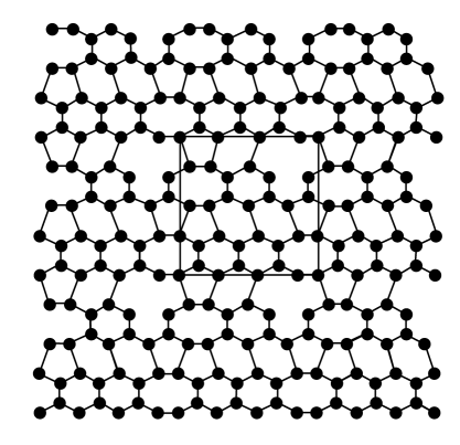
Thus, four-fold coordination was possible, but not favoured energetically. A typical metastable configuration is shown in fig. 1. The binding energy of such deep-lying minima was in the range of $-6.0$ to $-6.5$ eV/atom. The (crystalline) ground state of an infinite system - without an underlying lattice - has a hexagonal structure similar to that of a graphite layer, with each atom surrounded by three equidistant neighbours. In the finite on-lattice system, most of the deep-lying minima encountered contained a certain amount of adjacent slightly flattened hexagons, irrespective of the density, with the flattening due to the underlying square lattice. Note that, owing to the periodic boundary conditions, there will be configurations which appear to be different, but are equivalent to one another as they are connected by translations and/or rotations of the system. In the present work, such configurations are identified as equivalent and counted only once.

Another issue that needs to be considered when placing the networks on a lattice is the mesh size dependence of the results, which should of course be negligible. Clearly, halving the lattice constant will lead to more states. But as long as the width of the energy interval $\delta E$ used in the investigation is such that these new configurations all lie within the interval $[E,E+\delta E]$, the change in the lattice parameter just adds a constant to the entropy. This corresponds to a parallel shift in a semi-logarithmic plot of the local density of states, and, as we shall see, does not affect our conclusions. We have ensured that this requirement is fulfilled reasonably well for our on lattice networks. Finally, one has to establish the connectivity of the configuration space. In our case, the neighbours of a given configuration are obtained by all possible moves of a single atom from its current position to one of the neighbour points of the lattice. With $N_{A}$ atoms we have in a $d$ dimensional square lattice $2dN_{A}$ neighbors for each configuration. There is of course an amount of arbitrariness in the choice of the elementary moves which define the connectivity of the landscape. We were guided by the simple physical consideration that a single move should involve a change of coordinates which is small, i.e. of order $a$. This seems reasonable considering that collective moves are associated to vibrational motion, and thus take place on time scale much shorter than those of interest here.

B Lid algorithm

The method chosen to investigate the energy landscape of the networks is the so-called lid algorithm. Here, we will only give a short summary of the basic procedure; a more detailed description of the algorithm and the problem-independent implementation we have used can be found in the literature [9, 20]. Note that the lid algorithm is only applicable for discrete configuration spaces; continuous energy landscapes require a modified approach, the so-called threshold algorithm [10, 11].

The central idea is to restrict the investigation of the configuration space to a set of smaller subregions, called pockets, which surround local energy minima. These pockets contain a few hundred to a few million states and can be explored exhaustively. The procedure is as follows: Starting from a minimum $x_{i}$, we list all the states that are accessible to a nearest neighbor random walk, which starts at $x_{i}$ and which is restricted to states of energy lower than a prescribed energy value $L_{k}$, henceforth called the ‘lid’. (By nearest neighbor random walk we mean a random walk in configuration space, whose steps consist of precisely the previously defined elementary moves). From the exhaustive listing, we can compute the the local densities of states $D(E;L_{k},x_{i})$ and the local density of minima $D_{M}(E;L_{k},x_{i})$ for states available below the lid $L_{k}$. Integrating $D(E;L_{k},x_{i})$ with respect to $E$ over the interval $[0,L_{k}]$ we obtain the number of available states $N(L_{k};x_{i})$, and by the same operation applied to $D_{M}(E;L_{k},x_{i})$ the number of available local minima $M(L_{k};x_{i})$. The search is repeated for successively higher lid values $L_{k+1}$, $L_{k+2}$, etc., and for as many other pockets as possible. Note that the pocket is delimited by energy barriers instead of some distance in configuration space from the starting minimum. This is a natural first choice of selecting a physically relevant region of configuration space, due to the presence of an Arrhenius factor $\tau_{esc}\propto\exp(L_{k}/T)$, in the time of escape out of the pocket. One would like to repeat the analysis starting from every local minimum within a given pocket. Since the number of local minima within a given pocket of decent size ($>10^{5}$ states) was already on the order of $10^{4}$, this was not possible, and the available computer time was instead used for a sampling over more pockets for a given cell size and density. The starting minima for these pockets were found by using either simulated annealing or an adaptation of the lid method itself.

III Results

In this section we first describe in some detail the features of the data obtained by the exhaustive investigations, and then discuss their links to the thermodynamical features of the model and of glasses.

A General features of the data

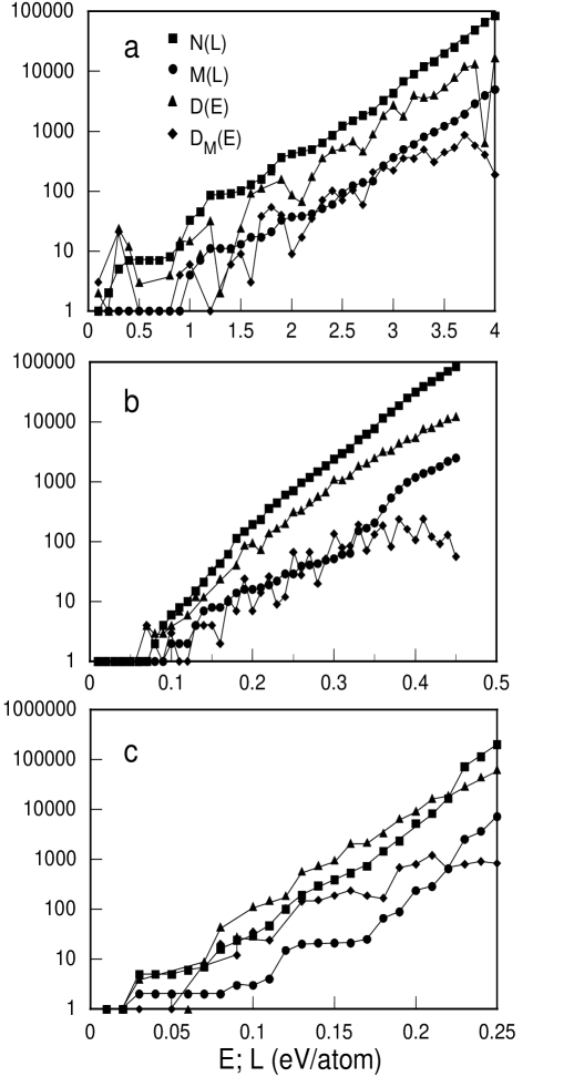
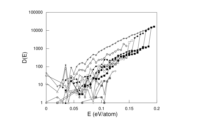
Figures 2a, 2b and 2c describe three different pockets, belonging to the systems $(N_{A}=22;S=12)$, $(N_{A}=36;S=16)$ and $(N_{A}=53;S=20)$ respectively. In each case we plot, on a semilogarithmic scale, $N(L)$ and $M(L)$ as functions of the lid $L$, and $D(E;L_{max})$ and $D_{M}(E;L_{max})$ as function of the energy $E$. For convenience, the dependence on $L_{max}$ of the last two functions is left understood. One notices the average exponential growth in all four quantities, with a flattening of $D(E)$ and $D_{M}(E)$ for energies near the maximum lid. Such a behaviour is exhibited in a large majority of the pockets, independent of (linear) size $S$ and density $\rho$.

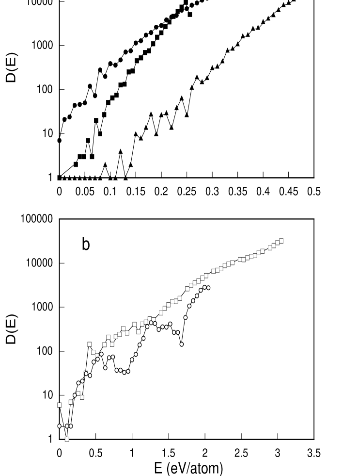
Figure  3 shows semi-logarithmic plots of the local density of states $D(E)$ for five different pockets belonging to systems of different cell sizes $S$ and different densities $\rho$ as indicated in the caption. These data are meant to illustrate the variations in the shape of $D(E)$ seen in the simulations. Note that the larger systems shown in the panel a) have a steeper growth of the local density of states than the smaller systems displayed in panel b). In the following we denote by $x_{i}$ the state of lowest energy within a certain pocket, and similarly by the index $i$ various other quantities associated with the pocket. In about 60% of all pockets studied the curves for $D(E)$ resembled those shown in (a1) (26%) or (a2) (34%), i.e. they exhibited simple exponential growth $D(E)=g_{i}\exp(E/E_{i})=g_{i}\exp(\alpha_{i}E)$, with $g_{i}=1$ and $g_{i}>1$, respectively. Here, $E_{i}=1/\alpha_{i}$ is the energy scale characterizing the exponential growth laws. In addition, the closely related case (b1) appeared for 29% of the pockets, while (a3) and (b2) represent some less common examples that occured in 3% and 8% of all cases, respectively. In some instances ((b1) and (a3)), the curves are best described by splitting them into two sections, each showing exponential growth, but with different ‘growth factors’ $\alpha_{i}(1)$ and $\alpha_{i}(2)$.

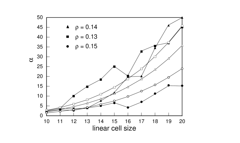
Figure 4 is a plot of $\alpha=<E_{i}>^{-1}$ versus the linear size of the cell, for different densities. Here the averaging is performed over all the pockets of systems with the same density $\rho$ and cell size $S$. It is clear that $\alpha$ increases and correspondingly $<E_{i}>$ decreases with decreasing density and increasing cell size. This result agrees qualitatively and to a certain extent also quantitatively with what one would expect from the simple free volume analysis [12] outlined in the appendix. To show the agreement, the calculated curves based on eq.6 for $\rho=0.13$, $0.14$ and $0.15$ are also depicted in figure 4 together with the actual data.

For a given value of $N_{A}$ and $S$ (considering only the larger pockets), one finds a considerable spread in the values of $E_{i}$, which vary up to a factor of two. This is quite different from the corresponding results obtained e.g. for spin glasses[21, 22], but it is consistent with the fluctuations of $N(L)$ and $D(E;L)$ around the average exponential growth curve. The size of the pockets and their local $DOS$ are quite variable, possibly because different spatially localized excitation patterns of the network can exhibit different growth behaviour in the associated $DOS$. Thus large side-basins with different growth laws can appear upon exceeding some energy barrier.

The density of minima shows a strong similarity to the density of states. Again, exponential growth is found, with the ratio of the growth factors $\alpha_{i}(D)/\alpha_{i}(D_{M})$ mostly in the range 1-2. This result agrees with the observation that the number of accessible states in a pocket $N(L)$ is more or less proportional to the number of minima $M(L)$, with the ratio $N(L_{m}ax)/M(L_{m}ax)$ mostly in the range $15-60$.

As a function of $L$, $N(L)/M(L)$ increases only slightly with the lid value. This holds true for all pockets investigated; and this observation is reflected in $M(L)$ running nearly parallel to $N(L)$ in a semi-logarithmic plot, once a lid value is reached where the first side-minima are accessible. Of course, $D_{M}(E;L_{max})$ eventually decreases, in most instances for energies close to the lid, $E\approx L_{max}$.

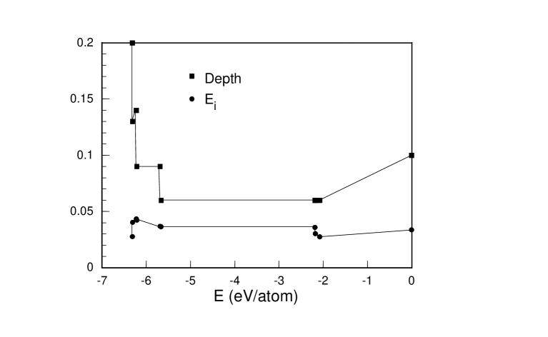
It is natural to investigate to what extent the properties of a pocket depend on the energy of its lowest energy state. Denoting as the depth of a pocket the smallest energy barrier which must be crossed in order to gain access to a lower minimum, we find that at least for larger pockets, $(N(L_{max})>1000)$, the depth grows as the energy of the lowest state decreases. With regard to the various growth factors, there exists a weak trend, insofar as pockets around low- energy minima tend to grow on the average slightly faster than the high-lying pockets, i.e. they have lower values of the $E_{i}$’s. However, many smaller pockets, often containing less than a dozen states and only a couple of minima, are interspersed among the larger ones along the energy-axis. Their depths do not appear to follow any particular pattern, but their growth quite closely follows an exponential law, analogous to the larger pockets.

B More detailed description of a typical example

Let us consider in some more detail a typical case such as the system with $(N_{A}=39,S=17)$. There are many local minima, each identified by its depth and by the energy of its lowest state. Each valley has its local density of states, which only includes states accessible by crossing energy barriers lower than the depth. All these local densities of states are to a good approximation exponential, and thus characterized by a growth rate, and its inverse $E_{i}$. Figure 5 shows a set of $E_{i}$’s (circles) and of depths (squares) plotted as function of the energy $E$ of the lowest state in the corresponding pockets. We see that the inverse growth rates do not vary much from pocket to pocket. The average value of $E_{i}$ is for this system $E_{gr}^{av}\approx 0.035\pm 0.005$ eV/atom. On the other hand, we note that pockets surrounding states of very low energy tend to be deeper than those surrounding less deep minima. In other words, the lower the energy the more rugged the landscape appears to be.

In addition, we show in fig. 6 for the ”ground state”- pocket ( ”ground state” = deepest minimum found on the energy landscape) the differences $\delta DOS(E;L_{k})$ between the densities of states for subsequent lid values $L_{k-1}$ and $L_{k}$. We note that these densities of states belonging to the added sub-regions at lid L are very similar up to the point of joining the main pocket. In particular, we note that at the lid $L=0.14$ eV/atom a large group of similar basins that are about as deep as the starting minimum join the main pocket. If one considers the growth factors of these $\delta DOS$, one finds $E_{i}^{av}(\delta DOS)\approx 0.027\pm 0.03$ eV/atom. These values are quite similar to the growth factor of the whole ”ground state”- pocket $(E_{i}\approx 0.028)$ eV/atom, and lie at the lower end of the range of growth factors shown in figure 5. Thus, the larger sub-basins added with increasing lid-size are quite similar to the pockets encountered during the sampling of the whole energy landscape.

C Configurational entropy

As mentioned in the introductory section, it is reasonable to discuss the excess entropy of the glass in terms of configuration space properties of network models. We have to assume that, at the temperatures of interest, the model system would thermalize in the pockets described by our numerical investigation. In this context, it is important to realize that the system experiences a qualitative change of behaviour at the temperature $T=E_{i}$. Analyzing the expectation value of the energy of a pocket with an exponentially growing density of states $D(E)\propto\exp(E/E_{i})$, one finds that for $T<E_{i}$, the system is trapped in the local minimum at the bottom of the pocket, i.e. the high barriers of the pocket keep the system isolated from the rest of the energy landscape. But for $T>E_{i}$, the system leaves the pocket with overwhelming probability, irrespective of the depth of the pocket. For a further discussion of exponential trapping and the competition among several exponential traps, see ref.[23].

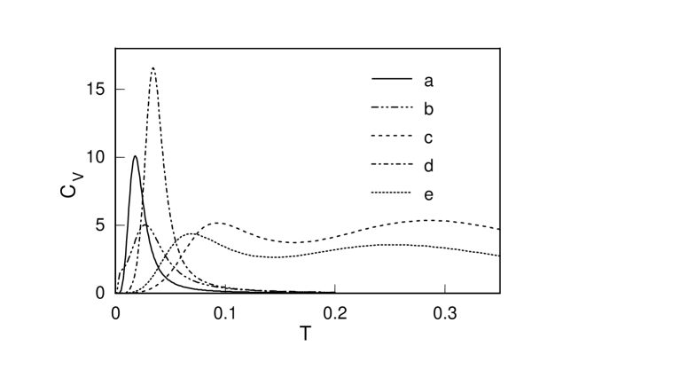
If the assumption of thermalization within the pocket holds true for $T\leq E_{i}$, all quasi-equilibrium properties of the system can be calculated by the usual formulae of statistical mechanics, but with the sums over states restricted to a pocket. As the local density of states is available, we can calculate average energies and heat capacities. The model specific heat was calculated for the example pockets shown in figure 3, and plotted as a function of $T$ in fig. 7. As one would expect, $C_{V}$ shows a clear maximum at a temperature close to the average inverse growth factor of the local density of states. The height of this peak is the larger, the larger the pocket is, and it is more pronounced the less the DOS deviates from an ideal exponential growth law. Note that deviations from a perfect exponential growth show up as additional features in $C_{V}$. In particular, a rapid exponential increase (with $E_{i}(1)$) of the DOS at low energies followed by a slower exponential growth (with $E_{i}(2)>E_{i}(1)$) (c.f. curves (b1) and (b2) in fig. 3b)) is reflected in a prepeak at $T\approx E_{i}(1)$ followed by the major peak at a temperature somewhat below $E_{i}(2)$ (curves (c) and (e) in fig. 7, respectively). .

A qualitatively similar behaviour of the excess specific heat $C_{p}$ is observed in a large number of glass-forming systems, ranging from molecular and polymer systems to metallic and covalent glasses [14]. Thus, the exponential growth of the local DOS of the network could be responsible for the configurational entropy observed in experiment. As a consequence, the glass transition would be the result of the system experiencing exponential trapping [23], with the glass transition temperature $T_{G}\approx E_{i}$. In this context, one should point out that the high- temperature tail ($T>E_{i}$) of the calculated specific heat of a pocket has no direct physical relevance when comparing the model with real glasses, since for $T>E_{i}$ the system would rapidly leave the pocket, and its equilibrium properties would no longer be dominated by the local density of states belonging to a single pocket.

This hypothesis of the thermodynamics of the glass transition being controlled by the trapping temperatures of locally ergodic, exponentially growing regions of the energy landscape of the glass raises the important question of the behaviour of the model system in the thermodynamic limit, $N_{A},V\rightarrow\infty$ with $\rho=N_{A}/V=const.$ Clearly, the number of possible neighbours of a configuration grows to infinity, and similarly the growth factor of the local $DOS$, i.e., the trapping temperature $E_{i}$ goes to zero. This follows from the fact that due to the short range of the covalent interactions the energetic barriers in the system would be expected to grow only with $V^{(d-1)/d}$, while the energy, as an extensive quantity, grows proportionally to $V$ itself. But one must not overlook the fact that there will be large entropic barriers preventing the system from exploring this infinite set of neighbouring states even though these are not separated by unsurmountable energetic barriers. From a certain point on, the system size has grown to such enormous proportions that the dynamics is controlled by entropic barriers, i.e. one is no longer allowed to assume that on the relatively short time scales available for observation the system can e.g. ”focus” all the thermal energy present in the network into a precise sequence of moves needed e.g. to cross some barrier to a neighbouring basin. Else, we would be on time scales where the glassy state can be transformed into the crystalline one, with the consequence that the configurational entropy vanishes, of course.

The existence of entropic barriers has important consequences for the dynamical behaviour of the system. Since the trapping temperature is a local equilibrium quantity of an exponentially growing region $\cal R$ of the energy landscape, it is necessary, in principle, to establish local ergodicity [12, 24] within $\cal R$, at temperatures below the trapping temperature. Usually, energetic barriers serve to delimit such regions, but in the thermodynamic limit entropic barriers fulfill this task. However, visualisation and characterization of such entropic barriers is usually not straightforward.

The simplest picture of entropic barriers with regard to the energy landscape would be to assume that the configuration space of the excitations of the (infinite) system can be approximately separated into a direct product of independent subspaces. Each such subspace can be treated in analogy to the independent modes of e.g. vibrations, and would usually be visualized as a ”cluster of atoms” within the network that has its individual excitation spectrum and corresponding density of states. Such clusters would be only weakly correlated with each other. Since the actual number of states within a pocket of the landscape of such a cluster is small compared to the number of clusters in an infinite system, the distribution of energy throughout the system equals a Poisson distribution over the clusters. In particular, the entropy $S(E,V,N)$ becomes an extensive function of the number of clusters $N_{C}$: $S(E,V,N)=N_{C}S_{C}$, where $E_{C}=E/N_{C},\;V_{C}=V/N_{C},\;$ and $N_{AC}=N_{A}/N_{C})$. The quantity $S_{C}$ is the entropy of a single cluster, and for an exponential density of states is proportional to $E_{C}/E_{i}$, similarly to the examples presented in this paper. If one now assumes that the glass transition is a consequence of the energy landscape consisting of (possibly nested) locally ergodic pockets (e.g. the ”clusters” discussed above) with exponentially growing densities of states, one would identify $T_{G}$ with the average inverse growth factor $E_{i}(V_{C})$ of such regions. Using the simple growth law ($E_{i}\propto 1/V$) derived in the appendix, such an identification yields an estimate of the size of these clusters. Since in the independent cluster approximation clusters of size $V_{C}$ suffice to describe many of the thermodynamic properties of the networks, this establishes a reasonable network size for structural investigations at the level of network topology.

In the case of 2d-networks, the trapping temperature for a $20\times 20$ system with $50-60$ atoms lies in the range of about $1eV(\approx 10^{4}K)$. Since the glass temperature for covalent networks lies in the range of $0.1eV(\approx 10^{3}K)$, the energy landscapes of networks with $N_{A}>500$ might be suitable for a realistic description of properties of glasses. While this number has been derived from the analysis of 2d-networks, preliminary results for 3d-networks indicate that the trapping temperature for e.g. networks with $40$ atoms lie at about $1.2$ eV/atom, leading again to an estimate of the needed network size of about $N_{A}>500$.

IV Conclusions

In this paper, we have presented a first in-depth study of the microscopic energy landscape of glasses at the level of their network topology. Such amorphous networks show an exponential growth of many important quantities, in particular the local density of states and minima, $D(E;L)$ and $D_{M}(E;L)$ respectively, the accessible state space volume $N(L)$ and the accessible neighbor-minima $M(L)$. This growth leads to exponential trapping that can explain the occurrence of a glass transition in such systems. In particular, the peak in the excess specific heat at the glass transition, that is often observed in experiments, follows directly from the exponential growth law.

This type of local exponential growth appears to be a common feature of many complex systems. Similar behaviour has been found for polymers [12, 25], spin glasses [21, 22, 26], combinatorial optimisation problems [9], crystalline solids [27, 28] and, in preliminary results by the present authors, for three-dimensional random networks.

It is expected that these results can form a more solid basis for phenomenological models of complex systems. An important open question is the issue of entropic barriers, since they control the effective size of locally ergodic pockets in large systems. Knowing this size would allow the direct quantitive comparison of the calculations with experimental data; e.g. one could predict the glass transition temperature and its dependence on cooling rates.

Acknowledgments
We gratefully acknowledge funding by the DFG via the SFB 408. This work was partly supported by a block grant from the Danish Statens Naturvidenskabelige Forskningsråd.

V Appendix

For the qualitative and semi-quantitative analysis of the network glasses, the following very simple free-volume-model that is based on some rough assumptions about the nature of the energy landscape can be helpful: 1. Starting from each configuration, $2dN_{A}$ new configurations can be generated by moving each atom to one of the $2d$ neighboring sites on the lattice ($d$ is the dimension of the lattice). 2. The interactions are highly local, such that the typical increase in energy $E_{M}$ of an acceptable move, i.e. one which leads to a configuration below the energy lid, is essentially independent of the number of atoms in the simulation cell. The typical increase in the energy/atom for a system with $N_{A}$ atoms when an acceptable move is performed is thus $E_{M}/N_{A}$. 3. As long as the states belong to the fast-growing region of the ”pocket”, the number of downhill moves among the acceptable moves will be very small. Thus we assume that a given move will result in a new configuration with an energy increase $\delta E\simeq E_{M}$ with a probability $f(\rho,N_{A})$. In particular, the probability $f_{-}$ for a downhill move should be very small compared to $f$, $f_{-}<<f$. Thus, the number of configurations $N(E+\delta E)$ with an energy below $E+\delta E$, is proportional to the number of configurations below the energy $E$, $N(E)$:

$$N(E+\delta E)\propto N(E)(2dN_{A}f)$$ (3)

from which it easily follows that

$$N(E)=N_{0}\exp(\alpha E),$$ (4)

with $\alpha=1/E_{i}=(1/E_{M})(2dN_{A}f-1)\approx 2dN_{A}f/E_{M}$. The last approximation should be acceptable in the limit $N_{A}\rightarrow\infty$ , as long as $f$ varies only weakly with $N_{A}$ (for fixed $\rho$).

It seems reasonable to assume that $f$ depends on the density of the system, and that it increases with the free volume per atom $v_{f}=V_{f}/N_{A}$ in the system, where the free volume $V_{f}$ is given in terms of the volume per atom $V_{A}$ as $V_{f}=V-N_{A}V_{A}$. Thus we get, for some constant $c$

$$f=cv_{f}=c(V-N_{A}V_{A})/N_{A}=c(V/N_{A})(1-\rho V_{A}),$$ (5)

and therefore

$$\alpha=1/E_{i}\approx 2dN_{A}f/E_{M}\propto V(1-\rho V_{A})$$ (6)

Equation 5 shows that $f$ increases with decreasing density for constant volume. Thus $E_{i}$ also decreases with density, and secondly, for constant density

$$E_{i}\propto 1/V.$$ (7)

This final result agrees quite well with the observed behaviour.

Note that according to eq.6, $E_{i}$ should actually decrease as $1/V(1-\rho V_{A})$. In order to check this behaviour, we need to determine $V_{A}$. This value corresponds to the number of lattice points that the atom would occupy in an energetically favourable configuration (recall that we are investigating the pockets around deep-lying minima). For an approximately hexagonal arrangement on the square lattice, we find $V_{A}=6$. If one plots $Y(=N_{A}E_{i})$ against $X(=1/(1-\rho V_{A}))$ for all available volumes $V=S^{2}(S=10,...,20)$ one finds that the data roughly follow straight lines as suggested by eq.6 [12].

Note that there exists only one free parameter $(c/E_{M})$ in this simple free volume model. The number of accessible states $N(L)$ estimated by this model exhibits an average exponential growth similar to $D(E)$ (c.f. fig. 2), and the qualitative dependence of the growth factors on $V=S^{2}$ and $\rho$ should be essentially the same for $D(E)$ and $N(L)$, unless e.g. there is a high degree of degeneracy in the ground state of the pocket. But even for polymer systems, where such a degenerate ground state occurs more frequently, an analogous free volume model roughly describes the dependence of the growth factors on system size [12, 25].

FIG. 1.: A typical network configuration belonging to a low-energy metastable state in a system of $27$ atoms with a unit cell of linear size $14$.

FIG. 2.: Number of accessible states $N(L)$ (squares), accessible minima $M(L)$ (circles), density of states $D(E)$ (triangles) and density of minima $D_{M}(E)$ ( diamonds) within a pocket, as a function of $L$ [eV/atom] and $E$ [eV/atom], respectively. Data are shown for three different pockets: a) $(N_{A}=22;S=12)$, b) $(N_{A}=36;S=16)$ and c) $(N_{A}=53;S=20)$.

FIG. 3.: Local density of states $D(E)$ vs. $E$ [eV/atom] for several representative systems: a): black squares (a1): $(N_{A}=46;S=18)$, black circles (a2): $(N_{A}=41;S=17)$, and black triangles (a3): $(N_{A}=34;S=16)$. b): white squares (b1): $(N_{A}=13;S=10)$ and white circles (b2): $(N_{A}=21;S=12)$. Note the curves belonging to the larger systems shown in a) are much steeper than those belonging to the smaller system shown in b).

FIG. 4.: The quantity $\alpha=1/<E_{i}>$ [1/(eV/atom)] for different densities: black squares: $\rho=0.13$, black triangles: $\rho=0.14$ and black circles: $\rho=0.15$. The white symbols show the corresponding theoretical predictions obtained through eq.6, with $V_{A}=6$. The average over the inverse growth factors $E_{i}$ is performed over all pockets in systems of the same density and cell size.

FIG. 5.: Depth (squares) and inverse growth factors $E_{i}$, both quantities expressed in $[eV/atom]$ for several sample pockets as a function of the lowest energy of the pocket. The system considered has $(N_{A}=39;S=17)$.

FIG. 6.: Local densities of states of several sub-basins of the ‘ground state’ pocket in the system $(N_{A}=39;S=17)$, which appear successively as the lid is raised. The top curve is the local density of states of the whole pocket. Note that the exponential trend is common to all sub-basins.

FIG. 7.: Specific heat in units of $[k_{B}]$ vs. temperature [eV/atom] calculated for several representative examples: a) $(N_{A}=46;S=18)$, b) $(N_{A}=41;S=17)$, c) $(N_{A}=13;S=10)$, d) $(N_{A}=34;S=16)$, and e) $(N_{A}=21;S=12)$. The three peaks in plots a), b) and d) are located at temperatures which match the inverse growth factors $E_{i}$ of the exponential density of states shown in Fig. 3a), (a1), (a2) and (a3), respectively. The double peaks of plots (c) and (e) correspond to the two different slopes characterizing the densities of states shown in Fig. 3b), (b1) and (b2), respectively.

REFERENCES

- [1] Landscape paradigms in Physics and Biology, Hans Frauenfelder, Alan R. Bishop, Angel Garcia, Alan Perelson, Peter Schuster, David Sherrington and Peter J. Swart Eds. Physica D 107, Nos. 2-4, 1996
- [2] C. Oligschleger and H. Schober. Solid State Comm., 93:1031, 1995
- [3] C. Oligschleger and J. C. Schön. J. Phys.:Cond. Matter., 9:1049, 1997
- [4] Simulation of Liquids and Solids, G. Ciccotti, D. Frenkel, and I.R. McDonald, Eds. North-Holland,Amsterdam, 1997
- [5] P. Vashishta, R. K. Kalia, J. P. Rino and I. Ebsjö. Phys. Rev. B., 41:12197, 1990
- [6] K. H. Hoffmann and P. Sibani. Phys. Rev. A, 38:4261, 1988, and references therein.
- [7] Jean-Philippe Bouchaud, Leticia F. Cugliandolo, Jorge Kurchan and Marc Mézard. cond-mat/9702070
- [8] K. Kremer and K. Binder. Comp. Phys. Rep., 7:259, 1988
- [9] P. Sibani, J. C. Schön, P. Salamon and J.-O. Andersson. Europhys. Lett., 22:479, 1993.
- [10] J. C. Schön, H. Putz and M. Jansen. J. Phys.:Cond. Matter., 8:143, 1996
- [11] J. C. Schön. Ber. Bunsenges. Phys. Chem., 100:1388, 1996
- [12] J. C. Schön. Habilitation Thesis., Univ. Bonn, 1997
- [13] Physics of Amorphous Materials, S. R. Elliott. Longman Scientific & Technical,Essex, 1990
- [14] The Vitreous State, I. Gutzow and J. Schmelzer. Springer,Berlin, 1995
- [15] W. A. Philipps. J. Low-Temp. Phys., 7:351, 1972
- [16] P. W. Anderson, B. I. Halperin and C. M. Varma. Phil. Mag., 25:1, 1972
- [17] Y. M. Galperin, V. L. Gurevich and D. A. Parshin. Phys. Rev. B, 32:6873, 1985
- [18] U. Buchenau, Y. M. Galperin, V. L. Gurevich and H. R. Schober. Phys. Rev. B, 43:5039, 1991
- [19] The Physics of Amorphous Solids, R. Zallen. Wiley,New York, 1983
- [20] P. Sibani, Ruud v.d. Pas and J. C. Schön in preparation
- [21] P. Sibani and P. Schriver. Physical Review B, 49:6667, 1994
- [22] P. Sibani. to appear in Physica A, 1998
- [23] J. C. Schön. J. Phys. A: Math. Gen. 30:2367, 1997
- [24] J. C. Schön and M. Jansen. in Pauling’s Legacy - Modern Modelling of the Chemical Bond, Z. B. Maksic and W. J. Orville-Thomas, Eds.. Elsevier, in press
- [25] J. C. Schön. preprint
- [26] T. Klotz, S. Schubert and K. Hoffmann. to appear in Europ. Journ. Phys. B
- [27] H. Putz, J. C. Schön and M. Jansen. Comp.Mater. Sci. in press 1998
- [28] M. A. C. Wevers, J. C. Schön and M. Jansen. preprint