Dynamics of Chainlike Molecules on Surfaces

Abstract

We consider the diffusion and spreading of chainlike molecules on solid surfaces. We first show that the steep spherical cap shape density profiles, observed in some submonolayer experiments on spreading polymer films, imply that the collective diffusion coefficient $D_{C}(\theta)$ must be an increasing function of the surface coverage $\theta$ for small and intermediate coverages. Through simulations of a discrete model of interacting chainlike molecules, we demonstrate that this is caused by an entropy-induced repulsive interaction. Excellent agreement is found between experimental and numerically obtained density profiles in this case, demonstrating that steep submonolayer film edges naturally arise due to the diffusive properties of chainlike molecules. When the entropic repulsion dominates over interchain attractions, $D_{C}(\theta)$ first increases as a function of $\theta$ but then eventually approaches zero for $\theta\rightarrow 1$. The maximum value of $D_{C}(\theta)$ decreases for increasing attractive interactions, leading to density profiles that are in between spherical cap and Gaussian shapes. We also develop an analytic mean field approach to explain the diffusive behavior of chainlike molecules. The thermodynamic factor in $D_{C}(\theta)$ is evaluated using effective free energy arguments, and the chain mobility is calculated numerically using the recently developed dynamic mean field theory. Good agreement is obtained between theory and simulations.

I Introduction

The dynamics of polymers on solid surfaces is an interesting theoretical problem that has important applications related to thin surface films. A central role in such systems is played by the diffusive dynamics of the chains. While the diffusion of adatoms and small molecules on surfaces is an extensively studied problem [1, 2], there are relatively few studies of the diffusion of more complicated molecules, and especially polymers on surfaces [3, 4, 5]. The pioneering experiments of George et al. [3] on short-chain alcanes on metal surfaces revealed that the coverage dependence of the collective diffusion coefficient $D_{C}(\theta)$ may show unusual features. For some molecules, it is approximately constant while for others, it is an increasing function of coverage for a wide range of values of $\theta$.

There has also been substantial interest recently on the spreading dynamics of molecularly thin oil films on solid substrates [6, 7, 8, 9, 10]. Many of these experiments are performed by depositing tiny, very flat droplets on surfaces. In the limit where the film becomes less than one monolayer in thickness, the spreading molecules are all in contact with surface forming a 2D molecular gas. In this regime, the dynamics of spreading and consequently the density profiles of the film edges are determined by the diffusion of the molecules. Experimental studies of spreading in the submonolayer regime [7, 8, 9] reveal that most of the measured film edge profiles are not well approximated by the Gaussian function but assume a steeper shape [11] that can be well fitted by a spherical cap in the rotationally symmetric case, i.e. droplet spreading [8, 9].

In the regime where the diffusion equation (Fick’s law) is a valid description, a non-Gaussian profile indicates that the collective diffusion constant $D_{C}(\theta)$ must have nontrivial coverage dependence. In the present context this was first realized in conjunction with the experiments of Albrecht et al. [8], where the observed spherical cap shaped droplets could be reproduced by Monte Carlo simulations of spreading of flexible chains in 2D. Analyzed in terms of Fick’s law with a coverage-dependent $D_{c}(\theta)$, it was concluded in Ref. [11] that $D_{c}(\theta)$ is a strongly increasing function of coverage up to $\theta\approx 0.4$ because of entropic repulsion between the chains.

In this work, our aim is to extend the work presented in Ref. [12] to carry out a systematic study of the spreading and diffusion of interacting chainlike molecules on surfaces. To begin with, we present an analysis of density profiles of spreading droplets with qualitatively different forms of $D_{c}(\theta)$. Using Fick’s law, we show how the spherical cap type of shapes result from the increase of $D_{c}(\theta)$ vs. $\theta$, and then quantitatively determine $D_{c}(\theta)$ from the experimental profiles of Ref. [8] up to $\theta\approx 0.4$. By extensive Monte Carlo simulations of a discrete model of interacting chainlike molecules, we then compute $D_{c}(\theta)$ for all coverages, and demonstrate that the chainlike nature of the molecules induces a strong repulsive interaction. When this dominates over interchain attractions, $D_{C}(\theta)$ first increases as a function of $\theta$ as deduced from the experiments, but eventually must go to zero for $\theta\rightarrow 1$. The relative maximum of $D_{C}(\theta)$ decreases for increasing attractions. We also examine the profiles of spreading droplets in detail for various interactions. For the case of pure entropic repulsion, we find excellent agreement between experimental and numerically obtained profiles. This demonstrates that steep density profiles can be obtained from energetic considerations without having to assume that the film edge acts as a phase boundary between a 2D condensate and a vapor phase, as suggested previously [9]. For increasing attractive interactions, the corresponding droplet shapes are in between spherical cap and Gaussian shapes.

Finally, we develop an analytic mean field approach to explain the behavior of the collective diffusion coefficient for chainlike molecules by using the fact that $D_{C}(\theta)$ can be expressed as the product of thermodynamic factor $\chi_{0}^{-1}$ and the mobility $m$. The thermodynamic factor is evaluated using effective free energy arguments, and the chain mobility is calculated numerically using the recently developed dynamic mean field theory [13]. Good agreement is found between theory and the numerical simulations.

The outline of the paper is as follows. In Sec. II we describe the analysis of spreading profiles from the diffusion equation which gives partial information about the collective diffusion coefficient. The lattice model used in this work is explained in Sec. III. The results of numerical simulations are presented in Sec. IV. We discuss briefly the results for athermal chains presented in Ref. [12], and present complete results for chains with attractive interchain interactions. In Sec. V we present the mean field theory for the thermodynamic factor $\chi_{0}^{-1}$ and the mobility $m$. In Sec. VI we use the chain-chain pair distribution function to extract the effective pair interaction potential for athermal chains. Finally, in Sec. VII we briefly summarize our main results.

II Analysis of Spreading Profiles from the Diffusion Equation

As discussed in the Introduction, experimental measurements of spreading density profiles of a polymer film in the submonolayer regime can be used to obtain information about the coverage dependence of the collective diffusion coefficient $D_{C}(\theta)$. This was first realized by Herminghaus et al. [11] who considered the spreading of polydimethylsiloxane (PDMS) on metal surfaces, including the data of Ref. [8]. A typical late-time spreading profile taken from this experiment is shown in Fig. 1. The height of the profile is measured in Ångstroms (Å), but it actually describes the average areal density distribution of polymers on the surface. As noted in Ref. [8], this and the other submonolayer profiles can be fitted very well with spherical cap function $\theta(x)=\theta_{0}+\sqrt{r^{2}-x^{2}}$ which is shown in Fig. 1 with a dotted line ($\theta_{0}$ and $r$ are fitting parameters). In the same figure we also show a Gaussian profile with a dashed line for comparison. While the shape of the profile clearly follows the spherical cap shape for most of the range of densities, at the lowest coverages the film edge displays a Gaussian shaped tail.

A qualitative way of analyzing the implications of the density profiles for $D_{C}(\theta)$ is to apply the non-linear diffusion equation [1, 11]

$$\frac{\partial\theta(x,t)}{\partial t}=\frac{\partial}{\partial x}\left[D_{C}(\theta)\frac{\partial\theta(x,t)}{\partial x}\right].$$ (1)

Starting from a delta function type of initial profile, the solution $\theta(x,t)$ of Eq. (1) is an exact Gaussian profile for all times when $D_{C}=const.$ In Fig. 2 we show typical results from the numerical solution of Eq. (1) for three choices of $D_{C}(\theta)$, including a monotonously decreasing and increasing functions of coverage $D_{C}(\theta)=1-0.99\theta$ and a $D_{C}(\theta)=0.01+0.99\theta$, respectively. For the first case, profiles are obtained that are below the Gaussians for high and intermediate coverages. On the other hand, for cases where $D_{C}(\theta)$ increases, profiles are above the Gaussian solution. This is exactly what was observed in the experiments (see Fig. 1) and thus we can conclude that $D_{C}(\theta)$ must be an increasing function of coverage for the range of covereges corresponding to the density profiles (see also Ref. [11]).

It is possible to determine $D_{C}(\theta)$ more quantitatively by solving density profiles from Eq. (1) and matching them with the experimental ones. We did this by using a fitting function for $D_{C}(\theta)$ of the form $D_{C}(\theta)=c_{1}+c_{2}\tanh[c_{3}(\theta-c_{4})]$, where $c_{1}$, $c_{2}$, $c_{3}$, and $c_{4}$ are fitting parameters. By adjusting these parameters it is relatively easy to obtain profiles with shapes closely matching the experimental ones of Ref. [8], with $c_{1}=0.159$, $c_{2}=0.144$, $c_{3}=5.174$, and $c_{4}=0.345$. The resulting profile is shown in Fig. 1 with a solid line. The matching of the profiles also fixes the normalized coverage scale from Fick’s law corresponding to the effective layer thickness in the experiments. The analysis reveals that $D_{C}(\theta)$ at very low concentrations is almost constant and then monotonically increases up to about $\theta=0.4$, in agreement with Ref. [11]. The resulting $D_{C}(\theta)$ from the best fits is shown in the inset of Fig. 1. We not that the behavior of $D_{C}(\theta)$ at higher values of $\theta$ cannot obtained from this procedure, because the maximum value of the experimental profile at hand is already less than $\theta=0.4$.

III Model of Chainlike Molecules

To determine $D_{C}(\theta)$ for all values of $\theta$ and to study the effects arising from the chainlike nature of the diffusing molecules on surfaces, we will in the present work use a discrete model called the fluctuating bond (FB) model [14]. This minimal model of polymers is widely used for simulations of many-chain systems [15]. The idea in the FB model is that it is a coarse-grained model of real polymer chains. Real polymers, such as simple polyethylene consist of repeated segments of ${\rm CH}_{2}$ monomers where carbon atoms are bound to each other forming a long chain. The bond length and the bond angle between adjacent carbon atoms are almost fixed. However, the torsional angle between adjacent bonds can have different values, and thus the end-to-end distance of a long chain of ${\rm CH}_{2}$ segments may vary significantly. On a coarse-grained level then, such a chain can be described by a reduced number of effective segments.

In the 2D version of FB model the chains in the model consist of connected segments that occupy sites on a square lattice. Each segment prohibits all other segments from occupying its nearest or next nearest neighbor lattice sites. In the model (see Fig. 3), the distance between adjacent segments $\ell$ can vary between $2\leq\ell\leq\sqrt{13}$ in lattice units, where the upper limit prevents bonds from crossing each other. With these restrictions there are 36 different bond vectors in the model. The FB model has been shown to give static properties, such as pressure, in full agreement with simulations of continuum models [16]. Furthermore, the FB model incorporates the same type of dynamics for a single chain as the continuum Rouse model [14].

To consider the general case where there are attractive interactions between the chains and the flexibility of individual chains can also vary, we have used the following Hamiltonian:

$$\frac{{\cal H}_{\rm eff}(r,\phi)}{k_{B}T}=\frac{4\epsilon}{k_{B}T}\sum_{l\neq l^{\prime}}^{n}\sum_{i,i^{\prime}}^{N_{FB}}\left[\left(\frac{\sigma}{r_{l,l^{\prime};i,i^{\prime}}}\right)^{12}-\left(\frac{\sigma}{r_{l,l^{\prime};i,i^{\prime}}}\right)^{6}\right]-\frac{E_{s}}{k_{B}T}\sum_{l=1}^{n}\sum_{i=1}^{N_{FB}-1}\cos(\phi_{l,i}).$$ (2)

In Eq. (2), the first term is a Lennard-Jones type of potential, where $J\equiv 4\epsilon/k_{B}T$ is the strength of the interaction, $r_{l,l^{\prime};i,i^{\prime}}$ is the distance between segments $i$ and $i^{\prime}$ of different chains $l$ and $l^{\prime}$, and $\sigma$ was chosen such that the potential minimum was at the distance of two in lattice units. The cut-off radius of the potential was $\sqrt{10}$ lattice units, after which the potential is small enough to give a negligible contribution. In the summations, $n$ is the number of chains and $N_{FB}$ is the number of segments in each chain. The second term controls the stiffness of each chain, with $\phi_{l,i}$ being the angle between two adjacent bonds $i$ and $i+1$ in chain $l$ and $K\equiv E_{s}/k_{B}T$ the stiffness parameter. For increasing $E_{s}$ or decreasing temperature $T$, the chains become more stiff.

Dynamics is introduced in the model by Metropolis moves of single segments, with a probability of acceptance $\min[e^{-\Delta{\cal H}_{\rm eff}/k_{B}T},1]$, where $\Delta{\cal H}_{\rm eff}$ is the energy difference between final and initial configurations for acceptable moves to a nearest neighbor site, for which site exclusion and bond length restrictions must be satisfied. One Monte Carlo (MC) time step is defined as an attempt to move each segment of every chain. In Fig. 3 we show a typical configuration of a chain in the FB model for $N_{FB}=6$. One possible move of a segment is shown by the dashed line. It should be noted that since the dynamics within the FB model consists of single segment moves only and there are no direct translational modes, the limit of a rigid rod is not well defined [17].

IV Numerical Simulations

A Athermal Chains

To quantitatively determine the coverage dependence of diffusion, we have performed extensive MC simulations using the FB model explained in Sec. III. First, we consider the case of fully flexible, athermal chains for which $J=K=0$ [12]. The linear size of the 2D square lattice we used was $L=180$ for most cases. To calculate $D_{C}(\theta)$ we used the temporal decay of the Fourier transformed density autocorrelation function $S(k,t)=S(k,0)e^{-k^{2}D_{C}(\theta)t}$, where $S(k,0)$ becomes constant in the hydrodynamic limit $k\rightarrow 0$. The density-fluctuation autocorrelation function is defined as $S(r,t)=\langle\delta\theta(r,t)\delta\theta(0,0)\rangle$, where $\delta\theta(r,t)\equiv\theta(r,t)-\langle\theta(r,t)\rangle$, and $S(k,t)$ is its Fourier transform [18]. It is calculated separately for each fixed value of the average normalized coverage $\theta\equiv\langle\theta(r,t)\rangle$ which for the FB model is defined to be $\theta=4nN_{FB}/L^{2}$. In Fig. 4 we show results of these calculations for the case $N_{FB}=6$ with circles. The results are normalized with $D_{1}$, which is the diffusion constant of a single monomer ($N_{FB}=1$) in the limit $\theta\rightarrow 0$. Initially, $D_{C}(\theta)$ increases up to $\theta\approx 0.7$, after which it rapidly approaches zero. The initial behavior of $D_{C}(\theta)$ is in good agreement with results obtained from the shape of the spreading profiles.

It is interesting to compare the behavior of $D_{C}(\theta)$ with the tracer diffusion coefficient of individual chains $D_{T}(\theta)$ defined by

$$D_{T}=\lim_{t\rightarrow\infty}{1\over 4tn}\sum_{i=1}^{n}\langle|\vec{r}_{i}(t)-\vec{r}_{i}(0)|^{2}\rangle,$$ (3)

where $\vec{r}_{i}(t)$ is the position vector of the $i^{\rm th}$ chain at time $t$. In Fig. 5 we show the results from simulations for the athermal case with circles. In the limit $\theta\rightarrow 0$ $D_{C}(0)=D_{T}(0)$, and thus we use the same normalization as in Fig. 4. As expected from increased interchain blocking, $D_{T}(\theta)$ is a monotonically decreasing function of $\theta$. This is a striking example of how fundamentally different the behavior of the two types of diffusion coefficients can be.

We have also studied the effect of chain length and stiffness to collective diffusion, and a summary of the results can be found in Ref. [12]. When the length of the chains increases diffusion slows down, but the relative maximum of $D_{C}(\theta)$ becomes more pronounced. With increasing stiffness diffusion slows down, too, but now the maximum of $D_{C}(\theta)$ becomes less pronounced.

B Chains with Attractive Interactions

To study the effect of attractive interactions between polymers we used the FB model with the Hamiltonian of Eq. (2) with two interaction parameters, namely $J=-0.5$ and $J=-1.0$. For the results presented here, we considered fully flexible chains ($K=0$) of length $N_{FB}=6$. The sizes of the lattices in the MC simulations varied from $100\times 100$ to $180\times 180$.

The results for the two cases as obtained from the decay of $S(k,t)$ are shown in Fig. 4. As the strength of the attractive interaction increases, diffusion slows down but the overall behavior as a function of $\theta$ is qualitatively similar to the athermal case. The main influence of the attraction is to significantly reduce the relative height of the maximum of $D_{C}(\theta)$ [19].

To compare with the athermal case, we also calculated $D_{T}(\theta)$ for which the results are shown in Fig. 5. When the strength of the interaction increases, $D_{T}(\theta)$ decreases more rapidly as a function of concentration.

C Spreading of Droplets

We also used the FB model to directly simulate the spreading of 2D submonolayer droplets. The chains were initially confined to a circular region, and after equilibration the spatial constraints were removed. The consequent spreading was monitored and corresponding density profiles calculated as a function of time. We find that within the accuracy of the fits, there is a linear relationship between the experimental and MC time scales which supports the use of the single-segment dynamics within the FB model.

In Fig. 6 we show a comparison between three experimental submonolayer profiles [8], profiles obtained from the MC simulations for athermal chains, and profiles computed using Eq. (1) with the tanh fitting function for $D_{C}(\theta)$ as explained previously. The agreement between all the profiles is excellent demonstrating the consistency of our approach. It also shows that the behavior of the PDMS polymers used in the experiment can be most simply explained in terms of athermal chain dynamics, with the entropic repulsion dominating. This is in contrast to the experiments of Ref. [9], where the steep film edges were assumed to be a 1D phase boundary between a 2D condensate and a vapor phase. Our results here demonstrate that no such assumptions need to be made; the steep spherical cap shapes of submonolayer droplets are expected to be a generic signature of strongly repulsive effective interactions.

In Figs. 7(a) and 7(b) we show additional spreading profiles for the cases $J=-0.5$ and $J=-1.0$, respectively. The changes seen in $D_{C}(\theta)$ in Fig. 4 can also be seen in the corresponding spreading profiles. In Figs. 7(a) and 7(b) the simulation results are shown with circles, a spherical cap fit with a solid line and a Gaussian fit with a dotted line. The main result is that with increasing attractive interactions, the shape of profiles changes from the spherical cap towards a Gaussian shape (except for the highest coverages). These results show the intimate connection between $D_{C}(\theta)$ and spreading profiles; in the regime where $D_{C}(\theta)$ is almost constant, the corresponding profile shape is close to the Gaussian limit.

V Mean Field Theory for Collective Diffusion

To better understand the somewhat unusual behavior of collective diffusion of chainlike molecules, we start from the Green-Kubo relation [1]

$$D_{C}=\lim_{t\rightarrow\infty}\frac{1}{2\langle(\delta n)^{2}\rangle}\int_{0}^{\infty}dt\langle\vec{J}(0)\cdot\vec{J}(t)\rangle\ ,$$ (4)

where $n$ is the number of chains, $\vec{J}(t)=\sum_{i=1}^{n}\vec{v}_{i}(t)$ is the total particle current, and $\langle(\delta n)^{2}\rangle$ the mean square fluctuation of chains (in a finite area $A$). In terms of the mean square displacements of the individual chains, this can be written as

$$D_{C} = \lim_{t\rightarrow\infty}\frac{\langle n\rangle}{\langle(\delta n)^{2}\rangle}\frac{1}{4tn}\left\langle\left(\sum_{i=1}^{n}\vec{r}_{i}(t)-\vec{r}_{i}(0)\right)^{2}\right\rangle$$ (5)

$$\equiv \chi_{0}^{-1}m,$$ (6)

where $\vec{r}_{i}(t)$ is the position of the center of mass of the $i^{\rm th}$ chain at time $t$. In this equation, the term $\chi_{0}^{-1}=\langle n\rangle/\langle(\delta n)^{2}\rangle$ defines the thermodynamic factor, and the remainder of the equation defines the mobility $m$. The thermodynamic factor is related to the density fluctuations of the system, while the mobility can be written as

$$m=\lim_{t\rightarrow\infty}\frac{n}{4t}\langle(\Delta\vec{r}_{CM})^{2}\rangle,$$ (7)

where $\Delta\vec{r}_{CM}=\vec{r}_{CM}(t)-\vec{r}_{CM}(0)$ is the displacement of the center of mass of all the chains, and $\vec{r}_{CM}(t)\equiv(1/n)\sum_{i=1}^{n}\vec{r}_{i}(t)$. In the theory presented here, we will treat the two factors $\chi_{0}^{-1}$ and $m$ separately.

A Thermodynamic Factor

To estimate the thermodynamic factor we consider a generalization of the simple thermodynamic theory presented for athermal chains in Ref. [12]. We take as a starting point an effective Helmholz free energy $F$ as

$$F=F_{0}-na\theta^{b}-k_{B}T\ln[\frac{n!}{(M-n)!n!}]-nk_{B}T\ln w.$$ (8)

The first term $F_{0}$ is a constant, while the second term $E_{int}=na\theta^{b}$ comes from attractive interactions between segments of different chains [1], and is temperature dependent. We calculated $E_{int}$ directly from the MC simulations at different coverages to estimate $a$ and $b$ and verified that this approximation is well satisfied. For the cases $J=-0.5$ and $J=-1.0$ the resulting values of these parameters are $a/k_{B}T=1.8$, $b=1.6$, and $a/k_{B}T=2.7$, $b=1.4$, respectively, while for the athermal case $a=b=0$. The third term comes from the entropy of the center of the mass of the $n$ polymers and it is here approximated by the expression for a 2D Langmuir gas on a lattice [1]. The parameter $M=L^{2}$ denotes the total number of lattice sites and thus $\theta=nN/M$ (for the FB model $\theta=4nN_{FB}/M$ due to the exclusion rules). The last term in Eq. (7) is the entropic contribution from the chainlike nature of the molecules, where $w$ is the number of possible configurations of each chain, and is a model dependent quantity. For the present case of chainlike molecules, we approximate it by decoupling the total number of configurations into the product of two terms

$$w(\theta)=w_{1}^{2}(\theta)w_{2}^{N-2}(\theta),$$ (9)

where $w_{1}(\theta)$ is the entropy arising from a segment at the end of the chain, and $w_{2}(\theta)$ from each segment in the middle of the chain. For the FB model with different interactions, we have numerically determined $w_{1}(\theta)$ and $w_{2}(\theta)$. In Fig. 8(a) we show the behavior of $w_{1}$ and $w_{2}$ with three different values of $J$, namely $J=0$, $J=-0.5$ and $J=-1.0$. These quantities can be easily interpolated for all coverages [20].

The chemical potential $\mu$ can be calculated from $F$ by using $\mu=(\partial F/\partial n)_{T,V}$ which gives

$$\frac{\mu(\theta)}{k_{B}T}=\frac{\mu_{0}}{k_{B}T}-a^{\prime}(b+1)\theta^{b}+\left[\ln\left(\frac{\rho}{1-\rho}\right)-\ln(w)\right],$$ (10)

where $\rho=\theta/N$ is the number of chain molecules per unit area with $N$ segments, and $a^{\prime}=a/k_{B}T$. It can be shown that the thermodynamic factor can be written as $\chi_{0}^{-1}=\theta[\partial(\mu/k_{B}T)/\partial\theta]$ [1], and thus we obtain

$$\chi_{0}^{-1}=1-a^{\prime}b(b+1)\theta^{b}+\frac{\theta}{N-\theta}-\theta\frac{\partial\ln(w)}{\partial\theta}.$$ (11)

In Fig. 8(b) the markers show results for $\chi_{0}^{-1}(\theta)$ as obtained from accurate MC simulations of the density fluctuations of the FB model (with $N_{FB}=6$) in equilibrium, as extrapolated to an infinite system size. At very high concentrations density fluctuations are so small that it is very difficult to obtain accurate results. Furthermore, with attractive interactions ($J\neq 0$) for coverages $\theta\mathchoice{\mathrel{\vbox{\hbox{$\buildrel\displaystyle>\over{\displaystyle\sim}$}}}}{\mathrel{\vbox{\hbox{$\buildrel\textstyle>\over{\textstyle\sim}$}}}}{\mathrel{\vbox{\hbox{$\buildrel\scriptstyle>\over{\scriptstyle\sim}$}}}}{\mathrel{\vbox{\hbox{$\buildrel\scriptscriptstyle>\over{\scriptscriptstyle\sim}$}}}}0.8$ the dynamics of the system slows down [19] and thus we here present results only for smaller coverages. Using the approximation of Eq. (11) with numerically determined $w_{1}(\theta)$ and $w_{2}(\theta)$ of Fig. 8(a) with $N_{FB}=N$ for the athermal case, the results show that the true magnitude of $\chi_{0}^{-1}(\theta)$ is somewhat underestimated throughout the range of coverages [12]. However, if the magnitude of the thermodynamic factor is known for some coverages, the effective chain length $N$ appearing in Eq. (9) can be used as an additional fitting parameter to improve the results. In Fig. 8(b) we show the results of this approach, with only one parameter $N$ fitted to our MC data for $\chi_{0}^{-1}(\theta)$. The corresponding values of the parameters for $J=-0.5$ and $J=-1.0$ are $N=11$, and $N=6$, respectively. For the athermal case $N=16$ gives the best results. Thus, for increasing attraction, the approximation of Eq. (9) seems to become more accurate.

B Calculation of Mobility

While the thermodynamic factor contains information about the equilibrium density fluctuations, the mobility $m$ is determined by the dynamics of the center-of-mass motion of the particles. To calculate $m$ theoretically we use the recently developed Dynamical Mean Field (DMF) theory [13], which yields an approximate expression for $m$ as

$$m_{\rm DMF}=\frac{\ell^{2}}{4}\Gamma,$$ (12)

where $\ell$ is the effective jump length and $\Gamma$ is the average jump rate. This formulation makes it very efficient to numerically evaluate $m$, and has recently been shown to give a very good approximation of the true $m$ for various strongly interacting systems [13].

In Fig. 9(a) we show mobilities calculated from MC simulations of $m(\theta)$ for the FB model for the cases $J=0$, $J=-0.5$ and $J=-1.0$, using the definition of Eq. (6). The data are normalized with the mobility of one segment $m_{1}$. In the same figure we show also the results calculated from the DMF theory of Eq. (12). The effective jump length $\ell$ has been estimated from the zero coverage limit, where $\chi_{0}(0)=1$ and thus $m_{1}=D_{1}$. In the athermal case the DMF theory is in good agreement with simulation results, but with increasing attraction between the chains it starts to deviate more from the MC simulation results. This behavior is physically reasonable, because attractive interactions strengthen the effect of dynamical correlations that are not included in the DMF theory [13]. Despite this, DMF gives the qualitative behavior of $m(\theta)$ rather well even in case of attractive chains.

A commonly used method to approximate the mobility is based on the Darken equation [1]. It states that the mobility can be approximated by the tracer diffusion coefficient, i.e. $m(\theta)\approx D_{T}(\theta)$. In Fig. 9(b) we show the complete results from simulations of $D_{T}(\theta)$ with the interaction parameters $J=0$, $J=-0.5$ and $J=-1.0$. In same figure, the markers denote the results of direct MC simulations of $m(\theta)$. As can be seen from the comparison, for the chainlike molecules $D_{T}(\theta)$ and $m(\theta)$ behave quite differently; for athermal chains even the curvatures of the two functions have opposite signs.

VI Effective Potential

The fact that the initial increase of $D_{C}(\theta)$ is due to effective repulsive interactions between the molecules can be seen in Eq. (10), where the important term $1-\theta[\partial\ln(w)/\partial\theta]$ comes from entropic origin of the chainlike molecules [11, 12]. With increasing attraction, this entropy-induced repulsion is compensated by the attractive $E_{int}$, and the maximum value of $D_{C}(\theta)$ is reduced in magnitude.

To study the effective potential corresponding to the entropic repulsion we calculated the chain-chain pair distribution function $g(r)=\sum_{ii^{\prime}}^{{}^{\prime}}\langle\delta(r-r_{i})\delta(r_{i^{\prime}})\rangle$ [21], where $r_{i}$ is the position of the center of mass of chain $i$ and prime indicates that terms with $i=i^{\prime}$ are to be omitted. From $g(r)$ we extracted numerically the effective pair interaction potential $V_{e}(r)/k_{B}T$ for athermal chains. This can be done by first calculating the direct correlation function $c(r)$ from the Ornstein-Zernike relation [22]

$$h(r)=c(r)+\theta\int h(r^{\prime})c(|r-r^{\prime}|)dr^{\prime},$$ (13)

where $h(r)=g(r)-1$ and $r$ is distance in lattice units. When $c(r)$ is known, $V_{e}(r)/k_{B}T$ can be calculated by using the hypernetted chain theory [23]

$$c(r)=-V_{e}(r)/k_{B}T+h(r)-\log[h(r)+1].$$ (14)

In Fig. 10 we show $V_{e}(r)/k_{B}T$ for the athermal case and for $\theta=0.25$, which shows a strong repulsion extending up to several lattice cites [24]. As a comparison in the same figure there is also a typical Lennard-Jones potential which is more repulsive at small distances. An interesting result of the analysis is that for athermal chains, all the computed pair correlation functions for coverages $\theta\leq 0.7$ and for several chain lengths [12] collapse to a single function which is given by $g(\tilde{r})=G(r\theta^{\alpha}/N_{FB}^{\beta})$, where $\alpha\approx 0.38$ and $\beta\approx 0.55$. These scaled correlation functions are shown in the inset of Fig. 10.

VII Discussion and Conclusions

In this paper we have presented a systematic study of diffusion and spreading of chainlike molecules, in part inspired by the non-Gaussian submonolayer film profiles observed in most experiments. Using Monte Carlo simulations with the fluctuating bond model, we have calculated the diffusion coefficients as a function of coverage, generalizing the results for athermal chains of Ref. [12] to chains with attractive interchain interactions. Typically, the collective diffusion coefficient $D_{C}(\theta)$ increases initially and displays a maximum around $\theta\approx 0.7$. The strength of the peak decreases with increasing attraction.

We have also developed a mean field approximation for the thermodynamic factor in $D_{C}$, while the mobility is estimated numerically from the Dynamical Mean Field theory. The theory reveals that the behavior observed in $D_{C}(\theta)$ is due to an entropy-induced repulsive interaction. We also extract this interaction numerically from the pair correlation functions for athermal chains. It is interesting to note that the diffusive dynamics of polymers in 2D is fundamentally different from the 3D case, where entanglement effects dominate in dense melts of longer chains [25].

The functional dependence of $D_{C}(\theta)$ on the coverage has interesting consequences for the profiles of spreading films in the submonolayer regime. When the entropy-generated repulsive interactions dominate, the droplets assume a spherical cap type of steep shape. Contrary to the suggestion of Ref. [9], no assumptions about the film edge being a phase boundary between a condensate and vapor need to be evoked here. With increasing attractive interactions these shapes evolve towars the Gaussian shape. If these interactions dominate and $D_{C}(\theta)$ is a deacreasing function of $\theta$, profiles emerge that are narrower than Gaussians. Thus, the submonolayer spreading experiments constitute a sensitive measure on the role of interactions in the diffusive dynamics of polymers on surfaces.

Acknowledgments: This work has in part been supported by the Academy of Finland.

                                   

FIG. 1.: A typical late-time submonolayer spreading profile from experiments of PDMS spreading on a silver surface [8] (filled circles). The height of the experimental profile is measured in Ångstroms (Å). Dashed and dotted lines are Gaussian and spherical cap fits, respectively. Solid line shows the solution of Eq. (1) using $D_{C}(\theta)$ shown in the inset. $D_{C}(\theta)$ has been normalized by the diffusion coefficient in the zero coverage limit $D_{C}(0)$.

                                   

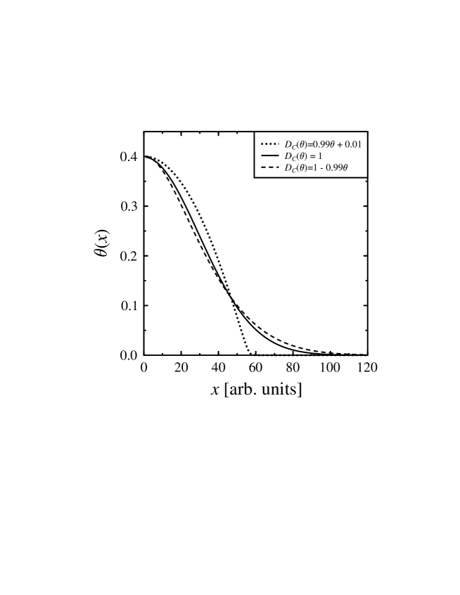
FIG. 2.: Typical results for the density profile of a droplet from numerical solutions of Eq. (1) with different choices of the function $D_{C}(\theta)$.

                                   

FIG. 3.: A typical configuration of a chain in the FB model with $N_{FB}=6$. The segments are shown by squares. Stars denote the sites blocked by the lowermost segment. An allowed move of one of the segments is shown by a dashed line.

                                   

FIG. 4.: $D_{C}(\theta)$ for three different values of $J$ as computed from MC simulations of the FB model. Circles are for $J=0$, squares for $J=-0.5$, and triangles for $J=-1.0$. Solid lines are only guides to the eye. The curves are normalized by the single monomer diffusion coefficient $D_{1}$ in the zero coverage limit. The error bars are of the size of the symbols, or smaller.

                                   

FIG. 5.: The tracer diffusion coefficient $D_{T}(\theta)$ for three different values of $J$. Circles are for $J=0$, squares for $J=-0.5$, and triangles for $J=-1.0$. Solid lines are only guides to the eye. The curves are normalized by the single monomer diffusion coefficient $D_{1}$. The error bars are smaller than the size of the symbols.

                                   

FIG. 6.: A comparison between three experimental submonolayer profiles measured after 50, 80, and 150 minutes following deposition of PDMS on silver [8, 12] (circles), MC simulations of 2D circular droplets from the FB model with $N_{FB}=6$ (squares), and numerical solutions of the nonlinear diffusion equation (solid lines). See text for details.

                                   

FIG. 7.: Typical spreading profiles obtained from the MC simulations with (a) $J=-0.5$ and (b) $J=-1.0$ circles. Solid and dotted lines denote spherical cap and Gaussian fits, respectively. The insets show simulated spreading profiles at three different times.

                                   

FIG. 8.: (a) Coverage dependence of $w_{1}(\theta)$ (three upper curves) and $w_{2}(\theta)$ (three lower curves) for $J=0$ (circles), $J=-0.5$ (squares), and $J=-1.0$ (triangles). Results of fitting [20] are shown by solid lines. In the zero coverage limit, both quantities have been computed numerically for a single fluctuating chain and thus do not depend on the value of $J$. (b) Calculated coverage dependence of $\chi_{0}^{-1}(\theta)$ for $J=0$ (circles), $J=-0.5$ (squares), and $J=-1.0$ (triangles). Solid lines show results of numerical calculations using Eqns. (8) and (10).

                                   

FIG. 9.: (a) Coverage dependence of $m(\theta)$ for $J=0$ (circles), $J=-0.5$ (squares), and $J=-1.0$ (triangles). The corresponding results from the DMF theory are shown by solid, dotted, and dashed lines, respectively. The data have been normalized by single segment mobility $m_{1}$ in the zero coverage limit. (b) Comparison between $m(\theta)$ and $D_{T}(\theta)$ with $m(\theta)$ plotted as in (a) and $D_{T}(\theta)$ shown for $J=0$ (solid line), $J=-0.5$ (dotted line), and $J=-1.0$ (dashed line).

                                   

FIG. 10.: Solid line shows the effective potential $V_{e}(r)/k_{B}T$ between the athermal chains in the FB model (see text for details). The dotted line denotes a typical Lennard-Jones potential for comparison. The inset shows seven scaled correlation functions $g(\tilde{r})$ for $N_{FB}=6$ and $\theta=0.25,\ 0.40,\ 0.50\ {\rm and}\ 0.75$, and for $N_{FB}=12$ and $\theta=0.25,\ {\rm and}\ 0.50$, and for $N=48$ the case $\theta=0.25$. See text for details.

REFERENCES

- [1] R. Gomer, Rep. Prog. Phys 53, 917 (1990).
- [2] T. Ala-Nissila and S. C. Ying, Prog. Surface Sci. 39, 227 (1992).
- [3] M. V. Arena, E. D. Westre, and S. M. George, J. Chem. Phys. 94, 4001 (1991), and references therein.
- [4] D. Cohen and Y. Zeiri, J. Chem. Phys. 97, 1531 (1992); Surface Sci. 274, 173 (1992).
- [5] K. A. Fichthorn, G. B. Prakash, and Y. Chen, Surface Sci. 317, 37 (1994); D. Huang, Y. Chen, and, K. A. Fichthorn, J. Chem. Phys. 101, 11021 (1994); K. A. Fichthorn, Adsorption 2, 77 (1996).
- [6] F. Heslot, N. Fraysse, and A. M. Cazabat, Nature 338, 640 (1989); A. M. Cazabat, N. Fraysse, F. Heslot, P. Levinson, J. Marsh, F. Tiberg, and M. P. Valignat, Adv. Coll. Int. Sci. 48, 1 (1994).
- [7] A. M. Cazabat, N. Fraysse, F. Heslot, and P. Carles, J. Phys. Chem. 94, 7581 (1990).
- [8] U. Albrecht, A. Otto, and P. Leiderer, Phys. Rev. Lett. 68, 3192 (1992); Surface Sci. 283, 383 (1993).
- [9] N. Fraysse, M. P. Valignat, A. M. Cazabat, F. Heslot, and P. Levinson, J. Coll. Int. Sci. 158, 27 (1993).
- [10] M. Haataja, J. A. Nieminen, and T. Ala-Nissila, Phys. Rev. E 52, R2165 (1995), and references therein.
- [11] S. Herminghaus, U. Sigel, U. Albrecht, and P. Leiderer, in Proceedings of the XVth Moriond Workshop “Short and Long Chains at Interfaces”, ed. by J. Daillont et al., Condensed Matter Physics Series, Villars-sur-Ollon, Switzerland, Jan. 21–28, 1995.
- [12] T. Ala-Nissila, S. Herminghaus, T. Hjelt, and P. Leiderer, Phys. Rev. Lett. 76, 4003 (1996).
- [13] T. Hjelt, I. Vattulainen, J. Merikoski, T. Ala-Nissila, and S.C. Ying, Surf. Sci. 380, L501 (1997).
- [14] I. Carmesin and K. Kremer, Macromolecules 21, 2819 (1988).
- [15] K. Binder, Monte Carlo and Molecular Dynamics Simulations in Polymer Science (Oxford University Press Inc., New York, 1995).
- [16] H. P. Deutsch and R. Dickman, J. Chem. Phys. 93, 8983 (1990).
- [17] As far as single chain dynamics is concerned, recent numerical studies using molecular dynamics [4, 5] reveal that diffusion of long chains cannot always be modeled as a single segment jumps from one site to another.
- [18] C. H. Mak, H. C. Andersen, and S. M. George, J. Chem. Phys. 88, 4052 (1988).
- [19] For the attractive cases, the chain configurations at coverages close to unity freeze into a glassy state and thus it becomes practically impossible to study diffusion with the present model.
- [20] For the cases and we used the fitting function and for we used . The corresponding parameters for the end segments for the cases , and were: ; ; and , respectively. The corresponding parameters for mid-segments were: ; ; and .
- [21] J. P. Boon and S. Yip, Molecular Hydrodynamics (Dover Publications Inc, New York, 1991).
- [22] L. Verlet, Phys. Rev. 165, 201 (1968).
- [23] J. P. Hansen and I. R. McDonald, Theory of Simple Liquids (Academic Press Inc., London, 1976).
- [24] The fact that direct repulsive interactions between pointlike particles typically cause to increase as a function of is well documented in the literature; see e.g. Refs. [1, 2].
- [25] M. Doi and S. F. Edwards, The Theory of Polymer Dynamics (Clarendon Press, Oxford, 1992).