Tensor product expansions for correlation in quantum many–body systems

Abstract

We explore a new class of computationally feasible approximations of the two–body density matrix as a finite sum of tensor products of single–particle operators. Physical symmetries then uniquely determine the two–body matrix in terms of the one–body matrix. Representing dynamical correlation alone as a single tensor product results in a theory which predicts near zero dynamical correlation in the homogeneous electron gas at moderate to high densities. But, representing both dynamical and statistical correlation effects together as a tensor product leads to the recently proposed “natural orbital functional.” We find that this latter theory has some asymptotic properties consistent with established many–body theory but is no more accurate than Hartee–Fock in describing the homogeneous electron gas for the range of densities typically found in the valence regions of solids. PACS 71.10.-w 71.15.Mb, Accepted for publication in Physical Review B

The fundamental difficulties associated with ab initio solutions of the quantum mechanical many–body problem stem directly from the large dimensionality of the wave function. Rather than dealing directly with the many–body wave function, large scale electronic structure calculations determine the ground–state energy by minimizing an energy functional over the much more manageable space of single–particle orbitals. Hohenberg–Kohn–Sham theory [1, 2] places this approach on a firm theoretical footing by establishing that exact electronic ground-state energies can be determined in this manner by minimizing a universal functional of such orbitals.

Although the requisite universal energy functional is not known exactly, the local density approximation[2] and various improvements thereon [3, 4, 5, 6, 7] are sufficient to resolve bond energies to a little better than one–tenth of an electron Volt. With this accuracy, these functionals make possible highly predictive first principles studies in diverse areas such as the study of surfaces, point defects, plastic deformation and chemical reactions. (For a review see[8].) Although sufficient for many studies, this error is too large to allow accurate prediction of the rates of microscopic processes at room temperature, thus limiting the ultimate predictive power of the ab initio density–functional approach. Whereas further improvement of energy functionals for single–particle theories is an active area of research, much less work has been done to construct energy functionals of the one–body density matrix[3, 9]. Such functionals are promising because the density matrix contains more explicit information than do the Kohn–Sham orbitals, and an accurate energy functional thus is likely to be simpler in form. The exact kinetic energy functional, for instance, is known for the density matrix, but not the Kohn–Sham orbitals.

To date, the only extensively used density–matrix energy functional is the Hartree–Fock approximation. One may view Hartree–Fock theory as approximating the two–body matrix as a sum of Hartree and exchange terms, each of which is a tensor product of the one–body density matrix. Hartree–Fock then uses the known, exact energy functional of the two–body density matrix to produce an energy functional of the one–body density matrix. In this work, we build upon this perspective and consider tensor product approximations to the two–body density matrix which not only serve as generators of energy functionals of the one–body density matrix but also provide estimates of the two–body matrix in terms of the one–body matrix and thereby shed light on the nature of correlation in quantum many–body systems.

Notation — For a system of $N$ electrons, the exact energy functional of the two–body density matrix $\gamma({{\bf x}_{1}}{{\bf x}_{2}},{{\bf x}^{\prime}_{1}}{{\bf x}^{\prime}_{2}})\equiv\langle\Psi|\hat{\psi}^{\dagger}({{\bf x}^{\prime}_{1}})\hat{\psi}^{\dagger}({{\bf x}^{\prime}_{2}})\hat{\psi}({{\bf x}_{2}})\hat{\psi}({{\bf x}_{1}})|\Psi\rangle/2$, is

$$E = \int d{{\bf x}_{1}}\left.\left(\left[-\frac{1}{2}\nabla^{2}_{{\bf r}_{1}}+U({{\bf r}_{1}})\right]n({{\bf x}_{1}},{{\bf x}^{\prime}_{1}})\right)\right|_{{{\bf x}^{\prime}_{1}}={{\bf x}_{1}}}$$ (2)

$$+\int d{{\bf x}_{1}}d{{\bf x}_{2}}\,\frac{\gamma({{\bf x}_{1}}{{\bf x}_{2}},{{\bf x}_{1}}{{\bf x}_{2}})}{|{{\bf r}_{1}}-{{\bf r}_{2}}|}.$$

Here and throughout, we work in atomic units, and the ${\bf x}_{i}$ are compound coordinates representing both position ${\bf r}_{i}$ and spin $s_{i}$ so that integration over ${\bf x}_{i}$ represents integration over space and summation over spin channels. The external potential and one–body density matrix are $U({\bf r})$ and $n({{\bf x}_{1}},{{\bf x}^{\prime}_{1}})\equiv\langle\Psi|\hat{\psi}^{\dagger}({{\bf x}^{\prime}_{1}})\hat{\psi}({{\bf x}_{1}})|\Psi\rangle$, respectively. Finally, the one–body density matrix comes directly from $\gamma$ through the sum–rule

$$\left(\frac{N-1}{2}\right)n({{\bf x}_{1}},{{\bf x}^{\prime}_{1}})=\int\!d{{\bf x}_{2}}\,\gamma({{\bf x}_{1}}{{\bf x}_{2}},{{\bf x}^{\prime}_{1}}{{\bf x}_{2}}).$$ (3)

Computational considerations — Although (2) is exact, the two–body density matrix $\gamma$ is a function of four variables, and direct computation with such functions is infeasible. Viable techniques, however, exist for dealing directly with two–variable functions such as the one–body density matrix[10, 11, 12, 13, 14, 15]. Accordingly, we expand $\gamma$ in terms of two–variable functions,

$$\hat{\gamma}=\sum_{i}\,\,\hat{g}_{i}\otimes\hat{h}_{i},$$ (4)

which, by separation of variables, is always possible. Here, $\hat{g}_{i}$ and $\hat{h}_{i}$ are one–body operators (functions of two variables), we view the two–body density matrix as a two–body operator (a function of four variables), and the tensor product denotes one of the three possible choices for separating four variables,

$$\hat{g}\hbox{\vbox{\hbox to10.0pt{\hfil$\otimes$\hfil}\hrule height=1.0pt,width=0.0pt\hbox to10.0pt{\hfil I\hfil}\hrule height=-5.0pt,depth=5.0pt}}\hat{h} = g({{\bf x}_{1}},{{\bf x}^{\prime}_{1}})h({{\bf x}_{2}},{{\bf x}^{\prime}_{2}})$$

$$\hat{g}\hbox{\vbox{\hbox to10.0pt{\hfil$\otimes$\hfil}\hrule height=1.0pt,width=0.0pt\hbox to10.0pt{\hfil II\hfil}\hrule height=-5.0pt,depth=5.0pt}}\hat{h} = g({{\bf x}_{1}},{{\bf x}_{2}})h({{\bf x}^{\prime}_{2}},{{\bf x}^{\prime}_{1}})$$

$$\hat{g}\hbox{\vbox{\hbox to10.0pt{\hfil$\otimes$\hfil}\hrule height=1.0pt,width=0.0pt\hbox to10.0pt{\hfil III\hfil}\hrule height=-5.0pt,depth=5.0pt}}\hat{h} = g({{\bf x}_{1}},{{\bf x}^{\prime}_{2}})h({{\bf x}_{2}},{{\bf x}^{\prime}_{1}}).$$

Quantum statistical considerations — We wish to maximize the physical content of a truncation of the expansion (4) to a limited number of terms. Physically, $n({{\bf x}_{1}},{{\bf x}^{\prime}_{1}})$ is the quantum amplitude for the insertion of a hole at position ${{\bf x}_{1}}$ and its instantaneous removal from ${{\bf x}^{\prime}_{1}}$, whereas $\gamma({{\bf x}_{1}}{{\bf x}_{2}},{{\bf x}^{\prime}_{1}}{{\bf x}^{\prime}_{2}})$ is the quantum amplitude for the insertion of a pair of holes at ${{\bf x}_{1}},{{\bf x}_{2}}$ and their removal from ${{\bf x}^{\prime}_{1}},{{\bf x}^{\prime}_{2}}$. Approximating the latter events as independent gives $\hat{\gamma}\approx\hat{\gamma}_{H}\equiv(\hat{n}\hbox{\vbox{\hbox to10.0pt{\hfil$\otimes$\hfil}\hrule height=1.0pt,width=0.0pt\hbox to10.0pt{\hfil I\hfil}\hrule height=-5.0pt,depth=5.0pt}}\hat{n})/2$, the familiar Hartree approximation, where the factor of two maintains the normalization implicit in (3). We may then refine this mean–field behavior and define $\hat{\gamma}\equiv\hat{\gamma}_{H}+\hat{\gamma}_{xc}$, where $\hat{\gamma}_{xc}$ represents exchange and correlation effects which we then expand, without loss of generality, according to (4).

The most significant drawback of the Hartree approximation is that $\gamma_{H}$ is not properly antisymmetric with respect to particle exchange (${{\bf x}^{\prime}_{1}}\leftrightarrow{{\bf x}^{\prime}_{2}}$), so that, potentially, many terms will be required in $\hat{\gamma}_{xc}$ to restore this symmetry. Alternately, we may explicitly ensure antisymmetry and take $\hat{\gamma}=\hat{\gamma}_{HF}+\hat{\gamma}_{c}\equiv(\hat{n}\hbox{\vbox{\hbox to10.0pt{\hfil$\otimes$\hfil}\hrule height=1.0pt,width=0.0pt\hbox to10.0pt{\hfil I\hfil}\hrule height=-5.0pt,depth=5.0pt}}\hat{n}-\hat{n}\hbox{\vbox{\hbox to10.0pt{\hfil$\otimes$\hfil}\hrule height=1.0pt,width=0.0pt\hbox to10.0pt{\hfil III\hfil}\hrule height=-5.0pt,depth=5.0pt}}\hat{n})/2+\hat{\gamma}_{c}$. In this form, $\hat{\gamma}_{HF}$ is precisely the familiar Hartree–Fock approximation. Again, we may expand the unknown $\hat{\gamma}_{c}$ as in (4).

Finally, we note that a fundamental difficulty exists when using a finite number of terms of Type II. Because of the instantaneous nature of the quantum event which $\gamma$ represents, we expect for normal systems that $\gamma\rightarrow 0$ as the insertion ${{\bf x}^{\prime}_{1}}{{\bf x}^{\prime}_{2}}$ and removal ${{\bf x}_{1}}{{\bf x}_{2}}$ locations are placed at ever further distances from one another. In an extended system with the expansion for $\gamma$ containing a finite sum of terms of Type II, taking this limit while keeping the insertion points near one another and the removal points near one another will violate this asymptotic condition unless each Type II term is identically zero. Accordingly, we focus below on approximating $\hat{\gamma}_{xc}$ and $\hat{\gamma}_{c}$ with terms of Type I and III.

Symmetry — Physical symmetries of $\hat{\gamma}$ significantly restrict the allowable forms for the tensor products appearing in expansions of the form (4) for $\hat{\gamma}_{xc}$ and $\hat{\gamma}_{c}$. We first consider Hermiticity $\gamma({{\bf x}_{1}}{{\bf x}_{2}},{{\bf x}^{\prime}_{1}}{{\bf x}^{\prime}_{2}})=\gamma^{*}({{\bf x}^{\prime}_{1}}{{\bf x}^{\prime}_{2}},{{\bf x}_{1}}{{\bf x}_{2}})$ and particle permutation symmetry $\gamma({{\bf x}_{1}}{{\bf x}_{2}},{{\bf x}^{\prime}_{1}}{{\bf x}^{\prime}_{2}})=\gamma({{\bf x}_{2}}{{\bf x}_{1}},{{\bf x}^{\prime}_{2}}{{\bf x}^{\prime}_{1}})$ for each of the three types of tensor product and defer discussion of Fermionic antisymmetry until after the sum–rule immediately below. Because both $\gamma_{H}$ and $\gamma_{HF}$ respect these symmetries, so must tensor products representing $\hat{\gamma}_{xc}$ and $\hat{\gamma}_{c}$. These symmetries imply relations with arbitrary constants of proportionality between the one–body operators of such products which may be absorbed into the one–body operators. Table I summarizes the final result of such considerations for all three tensor products. We note that in all cases symmetry restricts the tensor product to involve only a single one–body operator which remains to be determined.

Sum–rule — Remarkably, when a single term satisfying Hermiticity and particle permutation is used to represent $\hat{\gamma}_{xc}$ or $\hat{\gamma}_{c}$, we can “invert” the sum–rule (3) and determine the two–body density matrix $\gamma$ in terms of the one–body matrix $n$. Inserting the resulting form for $\gamma$ into (2) then generates an energy functional of the one–body matrix which implicitly satisfies the sum–rule, an important property for obtaining good ground state energies.

When terms of Type I represent $\hat{\gamma}_{xc}$ or $\hat{\gamma}_{c}$, the sum rule becomes $\hat{g}(\hbox{Tr\,}\hat{g})=\hat{o}$, where $\hat{o}=$ $\hat{n}$ or $\hat{n}(1-\hat{n})$, respectively. The solution of this equation is $\hat{g}=\pm\hat{o}/\sqrt{\hbox{Tr\,}\hat{o}}$. In either case, the extensivity of $\hbox{Tr\,}\hat{o}$ makes the resulting solution irrelevant in the thermodynamic limit $N\rightarrow\infty$. For products of Type III, the sum–rule combined with appropriate symmetries gives $\hat{g}^{2}=\hat{o}$, so that $\hat{g}=\sqrt{\hat{o}}$ with $\hat{o}$ defined as above.

Fermionic antisymmetry — Fermionic antisymmetry, $\gamma({{\bf x}_{1}}{{\bf x}_{2}},{{\bf x}^{\prime}_{1}}{{\bf x}^{\prime}_{2}})=-\gamma({{\bf x}_{1}}{{\bf x}_{2}},{{\bf x}^{\prime}_{2}}{{\bf x}^{\prime}_{1}})$, is a stronger condition than the particle permutation symmetry condition considered above and imposes more complex constraints. Two–body density matrices $\gamma$ which satisfy this condition may always be written with Type I and III products appearing in corresponding pairs of the form $\hat{g}\hbox{\vbox{\hbox to10.0pt{\hfil$\otimes$\hfil}\hrule height=1.0pt,width=0.0pt\hbox to10.0pt{\hfil I\hfil}\hrule height=-5.0pt,depth=5.0pt}}\hat{g}-\hat{g}\hbox{\vbox{\hbox to10.0pt{\hfil$\otimes$\hfil}\hrule height=1.0pt,width=0.0pt\hbox to10.0pt{\hfil III\hfil}\hrule height=-5.0pt,depth=5.0pt}}\hat{g}$ and with Type II products (were we to consider such) whose one–body terms are separately antisymmetric.

The two viable functionals remaining after the above considerations involve a Type III representation for either $\hat{\gamma}_{xc}$ or $\hat{\gamma}_{c}$. Unfortunately these forms do not consist of symmetric pairs of Type I and Type III products. To satisfy antisymmetry, one could take $\hat{\gamma}_{xc}=-(\hat{n}\hbox{\vbox{\hbox to10.0pt{\hfil$\otimes$\hfil}\hrule height=1.0pt,width=0.0pt\hbox to10.0pt{\hfil III\hfil}\hrule height=-5.0pt,depth=5.0pt}}\hat{n})/2$, so that $\hat{\gamma}=(\hat{n}\hbox{\vbox{\hbox to10.0pt{\hfil$\otimes$\hfil}\hrule height=1.0pt,width=0.0pt\hbox to10.0pt{\hfil I\hfil}\hrule height=-5.0pt,depth=5.0pt}}\hat{n}-\hat{n}\hbox{\vbox{\hbox to10.0pt{\hfil$\otimes$\hfil}\hrule height=1.0pt,width=0.0pt\hbox to10.0pt{\hfil III\hfil}\hrule height=-5.0pt,depth=5.0pt}}\hat{n})/2$, which is simply the Hartree–Fock approximation. To go beyond this, antisymmetry requires representing $\hat{\gamma}_{c}$ as a pair of terms so that $\hat{\gamma}=(\hat{n}\hbox{\vbox{\hbox to10.0pt{\hfil$\otimes$\hfil}\hrule height=1.0pt,width=0.0pt\hbox to10.0pt{\hfil I\hfil}\hrule height=-5.0pt,depth=5.0pt}}\hat{n}-\hat{n}\hbox{\vbox{\hbox to10.0pt{\hfil$\otimes$\hfil}\hrule height=1.0pt,width=0.0pt\hbox to10.0pt{\hfil III\hfil}\hrule height=-5.0pt,depth=5.0pt}}\hat{n}+\hat{g}\hbox{\vbox{\hbox to10.0pt{\hfil$\otimes$\hfil}\hrule height=1.0pt,width=0.0pt\hbox to10.0pt{\hfil I\hfil}\hrule height=-5.0pt,depth=5.0pt}}\hat{g}-\hat{g}\hbox{\vbox{\hbox to10.0pt{\hfil$\otimes$\hfil}\hrule height=1.0pt,width=0.0pt\hbox to10.0pt{\hfil III\hfil}\hrule height=-5.0pt,depth=5.0pt}}\hat{g})/2$.

The sum–rule for this latter extension on Hartree–Fock is $\hat{g}^{2}-\hat{g}(\hbox{Tr\,}\hat{g})=\hat{n}(1-\hat{n})$, which has no solution for $\hat{g}$ in extended systems unless $\hbox{Tr\,}\hat{g}$ vanishes in the thermodynamic limit. Under this condition, we have the solution $\hat{g}=\pm\sqrt{\hat{n}(1-\hat{n})}$, where the signs of the eigenvalues in the square root must be chosen to ensure $\hbox{Tr\,}\hat{g}=0$. For the paramagnetic phase we consider below, the natural choice is to take the upper sign for the spin–up block of the density matrix and the lower sign for the spin–down block. The structure of the energy functional (2), however, is such that for this choice the resulting energy functional of $\hat{n}$ is equal to that generated by representing $\hat{\gamma}_{c}$ as a single Type III product.

Representation of the functionals — The above discussion leaves the energy of two representations of the two–body matrix to explore: corrected Hartree theory, $\hat{\gamma}=\hat{\gamma}_{H}-(\sqrt{\hat{n}}\hbox{\vbox{\hbox to10.0pt{\hfil$\otimes$\hfil}\hrule height=1.0pt,width=0.0pt\hbox to10.0pt{\hfil III\hfil}\hrule height=-5.0pt,depth=5.0pt}}\sqrt{\hat{n}})/2$, and corrected Hartree–Fock theory, $\hat{\gamma}=\hat{\gamma}_{HF}-(\sqrt{\hat{n}(1-\hat{n})}\hbox{\vbox{\hbox to10.0pt{\hfil$\otimes$\hfil}\hrule height=1.0pt,width=0.0pt\hbox to10.0pt{\hfil III\hfil}\hrule height=-5.0pt,depth=5.0pt}}\sqrt{\hat{n}(1-\hat{n})})/2$. The corresponding energy functionals may be represented either directly in terms of the one–body density matrix for use with direct density-matrix methods[10, 11, 12, 13, 14, 15], or in terms of the spectral (“natural orbital”) representation of the density matrix.

The energy functional (2) contains one–body terms which may be evaluated directly in terms of the one–body density matrix. The remaining two–body term may be computed in terms of the two–point density $c({{\bf r}_{1}},{{\bf r}_{2}})\equiv\sum_{s_{1}s_{2}}\gamma({{\bf x}_{1}}{{\bf x}_{2}},{{\bf x}_{1}}{{\bf x}_{2}})$. When the above functionals represent paramagnetic states, this density has the following form in terms of the eigenvectors (natural orbitals) $\phi_{i}$ and corresponding eigenvalues (occupancies) $f_{i}$ of the one–body density matrix $\hat{n}$,

$$c({{\bf r}_{1}},{{\bf r}_{2}}) = {1\over 2}\left[4\sum_{ij}f_{i}f_{j}\phi_{i}({{\bf r}_{1}})\phi_{i}^{*}({{\bf r}_{1}})\phi_{j}({{\bf r}_{2}})\phi_{j}^{*}({{\bf r}_{2}})\right.$$ (6)

$$\left.-2\sum_{ij}g_{ij}\phi_{i}({{\bf r}_{1}})\phi_{i}^{*}({{\bf r}_{2}})\phi^{*}_{j}({{\bf r}_{1}})\phi_{j}({{\bf r}_{2}})\right],$$

where for corrected Hartree and Hartree–Fock theories, we take $g_{ij}=\sqrt{f_{i}f_{j}}$ and $g_{ij}=f_{i}f_{j}+\sqrt{f_{i}(1-f_{i})f_{j}(1-f_{j})}$, respectively.

The first of the above forms corresponds to the natural orbital functional proposed by Goedecker and Umrigar [3] as an ansatz among the many possible choices for the $g_{ij}$ which satisfy the sum–rule. Here, we see that this form is the unique Type III correction to Hartree theory which satisfies basic symmetries and the sum–rule. This theory has been studied analytically in the case of the homogeneous electron gas in the low density regime ($r_{s}>5.77$)[19]. Here, we present results for both this theory and our new corrected Hartree-Fock theory over a range of densities which includes both this low density regime and the regime more physically relevant in the valence region of solids, $r_{s}<5.77$.

Homogeneous electron gas — Translational invariance in the homogeneous gas ensures that the natural orbitals are plane waves. The remaining freedom in $\hat{n}$ lies in the occupancy eigenvalues $f_{\bf k}$. For the paramagnetic phase, the energy (2) then takes the following form,

$$E = 2\int\!{Vd{\bf k}\over(2\pi)^{3}}{{{\bf k}^{2}\over 2}f_{\bf k}}-{1\over V}\int\!{V^{2}d{\bf k}d{\bf k^{\prime}}\over(2\pi)^{6}}g_{{\bf k}{\bf k^{\prime}}}{4\pi\over|{\bf k}^{\prime}-{\bf k}|^{2}},$$ (7)

where $V$ is the volume of the system and the factor of two in the kinetic energy arises from the sum over spin.

The minimum of this energy functional occurs when ${\delta(E-\mu N)/\delta f_{\bf k}}=0$. For both corrected Hartree and corrected Hartree–Fock, this gives to leading order as $|k|\rightarrow\infty$,

$${\delta(E-\mu N)/\delta f_{\bf k}}\sim k^{4}-C/\sqrt{f_{\bf k}},$$

where $C$ is a constant. Hence, for large $k$, the momentum density scales as $f_{\bf k}\sim|{\bf k}|^{-8}$, in agreement with the random phase approximation and other many–body calculations[16]. This analysis holds for the present two functionals at all particle number densities and, in fact, for all theories of the form of (7) in which $g_{{\bf k}{\bf k^{\prime}}}\rightarrow\sqrt{f_{\bf k}f_{\bf k^{\prime}}}$ as $k\rightarrow\infty$ and $f_{\bf k}\rightarrow 0$.

Numerical Results — To determine the total energy of the homogeneous electron gas within the corrected Hartree and Hartree–Fock approximations, we exploit spherical symmetry and reduce $f_{\bf k}$ to a single variable function $f(k)$, which we represent on a radial mesh of variable spacing. We then minimize (7) with conjugate–gradients techniques subject to both the constraint that $f(k)$ corresponds to a total of $N$ electrons and the Fermi constraint that $0\leq f(k)\leq 1$. The latter constraint we implement by defining $f(k)\equiv(e^{-x}+1)^{-2}$, where $x$ is then free to range over the real line.

To evaluate the energy functional in terms of the fillings, we integrate numerically the kinetic and exchange–correlation terms in (7). A key step in producing accurate results is to avoid numerical integration across the familiar logarithmic singularity at $k=k^{\prime}$. For corrected Hartree theory, we avoided this by integrating the exchange–correlation terms once by parts analytically and then evaluating the result numerically. For the corrected Hartree–Fock case, we found it more efficient to approximate the Coulomb potential by a Yukawa potential, $e^{-\kappa r}/r$, and numerically extrapolate the results to $\kappa=0$. For these latter calculations, we found it more efficacious to work in the grand canonical ensemble (holding the chemical potential fixed while minimizing $E-\mu N$) than to impose the particle–number constraint explicitly.

The above procedures introduce four sources of numerical error: the finite spacing of the radial mesh, the finite extent of the mesh in $k$–space, the error in the extrapolation in the case of using the Yukawa potential, and the finite number of iterations involved in our searches for the minima. Through analysis and numerical experiments, we determine these errors to be less than $10^{-3}$, $10^{-4}$, $10^{-3}$ and $10^{-6}$ Hartree per particle, respectively, over the range of densities which we explored ($0.01<r_{s}<30$).

We found the minimization of the above functionals problematic for two reasons. First and foremost, the discretized representation of the one–dimensional function $f(k)$ on the radial mesh artificially stabilizes any discontinuities in $f(k)$ which may arise during the minimization process. This may be managed by taking care to ensure that the radial mesh provides sufficient resolution to describe any large gradients which arise in $f(k)$. An additional factor making the calculations difficult is that both the corrected Hartree and corrected Hartree–Fock functionals suffer from a very large condition number (in excess of $10^{7}$).

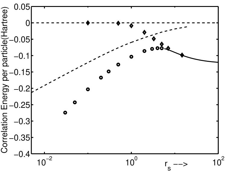
FIG. 1.: Correlation energy per particle of the uniform electron gas. Hartree–Fock (horizontal dashed line); exact many-body results[17, 18] (dashed curve), corrected Hartree theory (open circles), corrected Hartree–Fock theory (diamonds), analytic results[19] for corrected Hartree theory in the low density limit (solid curve).

Figure 1 compares our results for the correlation energy per particle of the electron gas with established many–body predictions. We find that at very low densities, both new theories begin to approach one another as $r_{s}\rightarrow\infty$. For even moderately low densities ($r_{s}>6$), both theories perform significantly worse than Hartree–Fock, overestimating the correlation energy by factors from two to four and higher. For the densities experienced in the valence regions of solids ($6>r_{s}>1$), corrected Hartree–Fock theory (diamonds) crosses over from over–correlation to under–correlation, whereas corrected Hartree theory (circles) over–correlates by roughly the same amount by which traditional Hartree–Fock theory under–correlates. For higher densities more representative of atomic cores ($1>r_{s}$), the corrected Hartree–Fock theory predicts near zero correlation. At these same densities, corrected Hartree theory remains over–correlated and gives a somewhat better estimate of the correlation energy than does traditional Hartree–Fock. The asymptotic form of the corrected Hartree results in the high density limit appears to be a straight line in our plot, which corresponds to the form of the leading order terms of the Gell–Mann–Brueckner expansion[20]. However, the prefactors which we find by a least squares fit, $E\approx 0.0570\log(r_{s})-0.0714$, are only correct to within a little better than a factor of two: the well–known analytic values for these coefficients are $0.0311$ and $-0.0480$, respectively. This suggests that the favorable reports for atoms for the natural orbital functional[3] may be in part a consequence of the high densities experienced in atomic cores, the limited particle number in the low density regions, and the self–interaction corrected nature of those calculations.

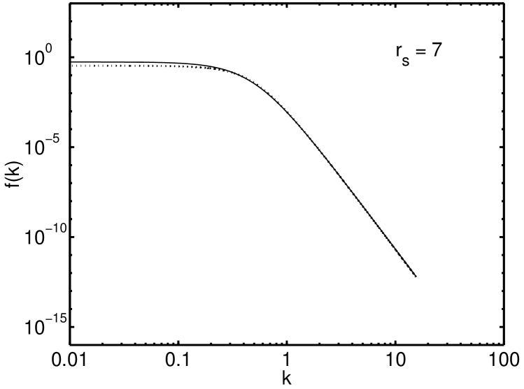
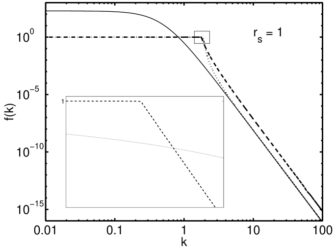
FIG. 2.: Predictions of momentum distribution of the uniform electron gas for $r_{s}=7$ and $r_{s}=1$: corrected Hartree theory (dashed curves), corrected Hartree–Fock theory (dotted curves), analytic results[19] for corrected Hartree theory in the low density limit (solid curve). Inset shows magnified view.

Figure 2 shows momentum distributions for $r_{s}=7$ and $r_{s}=1$, which are representative of what we find at low and high densities, respectively. We note that the numerical results of both theories exhibit the correct $k^{-8}$ scaling at large momenta and that we have very good agreement with the analytic results for the natural orbital functional[19] (applicable for $r_{s}>5.77$).

We observe that at low densities the momentum distributions of both corrected Hartree theory and corrected Hartree–Fock theory resemble one another quite closely and, in fact, approach one another as $r_{s}$ approaches infinity. This occurs because in this limit both theories predict very low occupations $f_{i}<<1$ so that the central quantities in the two theories approach one another, $f_{i}f_{j}+\sqrt{f_{i}(1-f_{i})f_{j}(1-f_{j})}\rightarrow\sqrt{f_{i}f_{j}}$.

The next panel of the figure illustrates that for densities outside the range of the applicability of the analytic solution ($r_{s}<5.77$), this solution predicts $f>1$ for sufficiently low momenta. We find that for such densities, the momentum distributions of corrected Hartree and corrected Hartree-Fock theory exhibit different behaviors at low momenta. Our numerical results indicate (to better than $1$ part in $10^{5}$) that the momentum distribution of corrected Hartree theory saturates to $f=1$ near the Fermi level. (See inset.) Such behavior is in direct contradiction of analytic and numerical many–body results for the electron gas[16, 18] and is contrary to the previously reported experience with atoms for this functional[3]. In contrast, the momentum distribution of corrected Hartree–Fock theory never saturates the Fermi occupation constraint, but rather approaches a value at $k=0$ which remains less than unity. We find that in the high density limit the corrected Hartree–Fock momentum distribution in fact approaches the standard Hartree–Fock result, ultimately leading to zero correlation energy for this theory in the high density limit.

In conclusion, we find that when the two–body density matrix is expanded beyond traditional Hartree and Hartree–Fock theories in terms of tensor products of one–body operators, fundamental symmetries allow the exchange–correlation hole sum–rule to be inverted to give estimates for the two–body matrix, and thus correlations, in terms of the one–body matrix. By approximating the two–body density matrix in terms of the one–body density matrix, this approach also leads to new energy functionals of the one–body density matrix.

The addition of the first separable term beyond Hartree theory shows some promising features when applied to the homogeneous electron gas, such as giving the correct scaling behavior of the momentum distribution in the high momentum limit and the correct scaling behavior of the correlation energy in the high density limit. However, the electronic states predicted by this functional are significantly over–correlated, and attempts to improve upon it by the addition of further terms without additional constraints would only add more freedom in the minimization and lead to further over–correlation. Hence, before adding a second term, it is important to use antisymmetry to constrain the first such term to be the traditional Fock term. This gives the second functional which we considered, corrected Hartree–Fock theory. This second theory under–correlates the electron gas in the high density limit but still over–correlates at lower densities. This indicates that the addition of further terms will only hold the promise of producing a more accurate functional if additional, appropriate constraints are imposed.

REFERENCES

- [1] P. Hohenberg and W. Kohn, Phys. Rev. 136, B864.
- [2] W. Kohn and L. J. Sham, Phys. Rev. 140, A1133 (1965).
- [3] S. Goedecker and C. J. Umrigar, Phys. Rev. Lett. 81, 866, (1998).
- [4] J.P. Perdew and W. Yue, Phys. Rev. B 33, 8800 (1986).
- [5] Y.M. Juan and E. Kaxiras, Phys. Rev. B 48, 14944 (1993).
- [6] G. Ortiz, Phys. Rev. B 45, 11328 (1992).
- [7] A. D. Becke, Phys. Rev. A 38, 3098 (1988).
- [8] M. C. Payne et al., Rev. Mod. Phys. 64 No. 4 (1992).
- [9] E. R. Davidson, Reduced Density Matrices in Quantum Chemistry, Academic Press, New York (1976)
- [10] F. Mauri et al., Phys. Rev. B 47, 9973 (1993).
- [11] X.-P. Li et al., Phys. Rev. B 47, 10891 (1993).
- [12] M. S. Daw, Phys. Rev. B 47, 10895 (1993).
- [13] P. Ordejon et al., Phys. Rev. B 51, 1456 (1995).
- [14] E. Hernandez and M. J. Gillan, Phys. Rev. B 51, 10157 (1995).
- [15] W. Kohn, Phys. Rev. Lett. 76, 3168 (1996).
- [16] B. Farid et al., Phys. Rev. B 48 11602, (1993)
- [17] G. D. Mahan, Many–Particle Physics, Plenum Press, New York, NY (1990).
- [18] D. M. Ceperley and B. J. Alder, J. de Physique C7 41 295 (1980); D. M. Ceperley and B J. Alder, Phys. Rev. Lett. 45 566 (1980).
- [19] J. Cioslowski and K. Pernal, J. Chem. Phys. 111 3396 (1999)
- [20] M. Gell–Mann and K. Brueckner, Phys. Rev. 106 364 (1957).