Variational theory for site resolved protein folding free energy surfaces

Abstract

We present a microscopic variational theory for the free energy surface of a fast folding protein that allows folding kinetics to be resolved to the residue level using Debye-Waller factors as local order parameters. We apply the method to $\lambda$-repressor and compare with site directed mutagenesis experiments. The formation of native structure and the free energy profile along the folding route are shown to be well described by the capillarity approximation but with some fine structure due to local folding topology.

Proteins fold on a configurational energy landscape that has the shape of a funnel [1]. As the protein moves down the funnel towards the native state, incomplete cancellation of the entropy and energy losses may result in free energy barriers. So far, proteins that fold fast exhibit single exponential kinetics [2], consistent with a free energy profile that has a single highest barrier along the progress coordinate. Central issues are the origin of the free energy barrier for fast folding proteins and how the ensemble of structures which represent the bottleneck is to be characterized. We address these questions using a variational approximation that describes ensembles of partially folded proteins at the highest level of resolution, i.e., the specific role of individual residues in guiding the protein to the native state is quantified. In the laboratory, Fersht has developed a probe of the transition state or bottleneck ensemble through protein engineering kinetic studies in which the sequence of the protein is altered by replacing residues one at a time[3]. The experiment yields the fraction of the time that the mutated site is in the native conformation in the bottleneck ensemble by comparing folding rates of the mutant to the wild type. Since this can be done for any residue in the sequence, these studies are inherently “site resolved”. Resolving the transition state ensemble to this level is one way to monitor the average of the many routes taken as proteins fold.

Previous analytic mean field theories and simulations have produced energy landscapes in one or two global dimensions characterizing the folding ensemble[4]. We develop here a free energy profile for proteins with a funneled landscape that is completely “site resolved”, i.e., one dimension per residue, by extending the mean field variational calculations presented in [5]. The underlying Hamiltonian explicitly incorporates chain stiffness and connectivity while the approximation employs a variational density that monitors local order parameters for folding akin to the Debye-Waller factors (also called temperature factors) for individual residues seen in X-ray crystallography.

The basic Hamiltonian for an interacting polymer chain is $H=H_{\rm chain}+H_{\rm int}$ where $H_{\rm chain}$ is backbone potential and $H_{\rm int}$ are the interactions between distant monomers along the chain. $H_{\rm chain}$ is an effective harmonic potential $\beta H_{\rm chain}=1/2\sum{\bf r}_{i}\cdot\Gamma_{ij}\cdot{\bf r}_{j}+B\sum{\bf r}_{i}^{2}$ where $\{{\bf r}_{i}\}$ are the positions of the $N$ $\alpha$-carbons, and $\beta=1/k_{B}T$ is the inverse temperature. The first term enforces the chain connectivity while the second term confines the radius of gyration to a reasonable value (achieved by fixing $B$ to a small constant: $B=3/2a^{2}\times 10^{-3}$). For the connectivity matrix, $\Gamma_{ij}$, we use the well known Gaussian approximation to the freely rotating chain derived in [6]. Denoting the $i^{th}$ bond vector by ${\bf a}_{i}=({\bf r}_{i+1}-{\bf r}_{i})$ and the angle between successive bond vector by $\theta$, this stiff chain model is defined by the correlations $\langle{\bf a}_{i}\cdot{\bf a}_{i+l}\rangle=a^{2}g^{l}$, where $a$ is the mean bond length and $g=\cos\theta$. Following Bixon and Zwanzig, $\Gamma_{ij}$ is determined by inverting these correlations and transforming to the bead representation resulting in a pentadiagonal matrix that depends on the stiffness parameter $g$; (for the explicit matrix, see [6]). In the limit $g\rightarrow 0$, $\Gamma_{ij}$ describes the standard flexible chain, whereas $g\rightarrow 1$ corresponds to a rigid rod. The persistence length, $l$, for this chain is given by $l=a/(1-g)$. We use $g=0.8$ giving (with $a=3.8{\rm\AA}$) $l\approx 20{\rm\AA}$, the persistence length for poly-L-alanine [7].

We take interaction between distant monomers along the chain to be restricted to specifically native-like interactions $H_{\rm int}=\sum\!^{(N)}\>\epsilon_{ij}u(|{\bf r}_{i}-{\bf r}_{j}|)$ where the isotropic pair potential, has a minimum at a non-zero distance produced by summing three Gaussians, $u(r)=\gamma_{s}e^{-\beta_{s}r^{2}}+\gamma_{i}e^{-\beta_{i}r^{2}}-\gamma_{l}e^{-\beta_{l}r^{2}}$; the short- and intermediate-range terms are repulsive while the long-range Gaussian is attractive $(\beta_{s}>\beta_{i}>\beta_{l})$. The sum over pair interactions $(\sum^{(N)})$ is restricted to native contacts. This constraint gives a smooth funnel shaped energy landscape, appropriate for fast folding proteins. This is an extreme realization of the principle of minimum frustration [8] and is reminiscent of the lattice model originally introduced by G$\bar{{\rm o}}$ [9]. The heterogeneity of the interaction between different residues is reflected by the strength $\epsilon_{ij}$. Non-native interactions can also be included in $H_{\rm int}$ and treated by our variational method.

To study the many dimensional free energy surface defined by $H$, we choose local order parameters that can characterize the ensemble of partially folded structures by specifying the temperature factor for each residue, $\hat{{\cal B}}_{i}$. This describes the mean square fluctuations of a residue about its native position and for fully folded proteins has been measured. A similar local order parameter for folding has been used in lattice simulations [10] and earlier analytical work [5]. Consider the free energy surface defined by the set of scalar fluctuations of each residue from its native position $\{{\bf r}_{i}^{N}\}$, $\hat{{\cal B}}_{i}=({\bf r}_{i}-{\bf r}_{i}^{N})^{2}$. The free energy surface ${\cal F}[\{\hat{{\cal B}}_{i}\}]$ for an ensemble specified by $\{\hat{{\cal B}}_{i}\}$ is given by

$$e^{-\beta{\cal F}[\{\hat{{\cal B}}_{i}\}]} = {\rm Tr}\;\left[\prod_{i}\delta\left(\hat{{\cal B}}_{i}-({\bf r}_{i}-{\bf r}_{i}^{N})^{2}\right)e^{-\beta H}\right]$$ (1)

$$= \int\!\!{\cal D}\lambda\>{\rm Tr}\;e^{-\beta H[\lambda]},$$ (2)

where $\beta H[\lambda]=\beta H+\sum\lambda_{i}(\hat{{\cal B}}_{i}-({\bf r}_{i}-{\bf r}_{i}^{N})^{2})$, and ${\cal D}\lambda\equiv\prod_{j}d\lambda_{j}/2\pi i$.

Denoting the integrand in Eq.(2) by $e^{-\beta F[\lambda]}$, we approximate $F[\lambda]$ with the help of a reference Hamiltonian $H_{0}$ and the Gibbs-Bogoliubov variational expression $F[\lambda]\approx-k_{B}T\log Z_{0}+\langle H[\lambda]-H_{0}\rangle_{0}$ , where $Z_{0}={\rm Tr}\left[e^{-\beta H_{0}}\right]$, and $\langle\cdots\rangle_{0}$ means the average with respect to $H_{0}$. The reference Hamiltonian describes a Gaussian chain constrained to fluctuate about the native structure $\{{\bf r}_{i}^{N}\}$ by a harmonic external field: $\beta H_{0}=H_{\rm chain}+\sum C_{i}({\bf r}_{i}-{\bf r}_{i}^{N})^{2}$. The variational parameters $\{C_{i}\}$ are conjugate to $\{\hat{{\cal B}}_{i}\}$. This reference Hamiltonian captures the two stable phases of fast folding proteins: the globule with small $\{C_{i}\}$ and the native state with uniformly large $\{C_{i}\}$. $\{C_{i}\}$ also form a set of local order parameters for folding. A similar (but more elaborate) reference Hamiltonian was used to determine the phase diagram for proteins with a rugged energy landscape as well as to study folding free energy barriers[5]. These mean field studies employed a global order parameter for nativeness by setting all ${C_{i}}$ equal in one region of the protein. Different related effective harmonic variational Hamilitonians have been employed to study polymers in random media[11], random directed polymers[12], and random copolymers [13].

Evaluating Eq.(2) using the steepest descents approximation gives the stationary condition $\hat{{\cal B}}_{i}=\langle({\bf r}_{i}-{\bf r}_{i}^{N})^{2}\rangle_{0}$ as a function of $\{C_{i}\}$ leading to a one to one relation between the $\{\hat{{\cal B}}_{i}\}$ and $\{C_{i}\}$. Technically, it is more convenient to study the free energy surface in $\{C_{i}\}$ space so that we consider the variational free energy surface expressed as $F[\{C_{i}\}]=E-ST$ with the estimate for the energy $E=\sum^{(N)}\epsilon_{ij}\langle u({\bf r}_{ij})\rangle_{0}$ and the entropy $S/k_{B}=\log Z_{0}+\sum\langle C_{i}({\bf r}_{i}-{\bf r}^{N}_{i})^{2}\rangle_{0}$ as a function of $\{C_{i}\}$.

Since $H_{0}$ is quadratic, $Z_{0}$ and all of the averages are expressible in terms of the correlations, $\langle{\bf r}_{i}\cdot{\bf r}_{j}\rangle_{0}-\langle{\bf r}_{i}\rangle_{0}\cdot\langle{\bf r}_{j}\rangle_{0}=3/2G_{ij}$, with $G_{ij}=\left[1/2\;\Gamma_{ij}+(B+C_{i})\delta_{ij}\right]^{-1}$. $Z_{0}$ involves the determinant of the correlation matrix while the averages can be calculated using the density of site $i$, $\rho_{i}({\bf r})=\langle\delta({\bf r}-{\bf r}_{i})\rangle_{0}$, and the pair density between sites $i$ and $j$, $\rho_{ij}({\bf r})=\langle\delta({\bf r}-{\bf r}_{ij})\rangle_{0}$. In terms of the average position ${\bf s}_{i}=\sum_{j}G_{ij}C_{j}{\bf r}_{j}^{N}$ these densities are $\rho_{i}({\bf r})=\left(\pi G_{ii}\right)^{-3/2}\exp\left[-({\bf r}-{\bf s}_{i})^{2}/G_{ii}\right]$, and $\rho_{ij}({\bf r})=\left(\pi\delta G_{ij}\right)^{-3/2}\exp\left[-({\bf r}-{\bf s}_{ij})^{2}/\delta G_{ij}\right]$ where $\delta G_{ij}=G_{ii}+G_{jj}-2G_{ij}$.

Since both $F[\{C_{i}\}]$ and $\nabla_{C}F[\{C_{i}\}]$ can be expressed analytically in terms of $G_{ij}$ (which is calculated numerically), it is relatively easy to locate the minima and saddle points numerically [14]. Once the transition states and the folded, unfolded, and local minima are determined, we define the average folding route to be the connected steepest descents path from each transition state to the neighboring minima. Only the global minimum of $F[\{C_{i}\}]$ is rigorously an upper bound but the saddle points and local minima should also be good estimates for the true free energy surface.

We now apply the model to the folding of the $\lambda$-repressor protein. $\lambda_{6-85}$ is a good candidate system since it is small (80 residues) and folds extremely rapidly in 20 $\mu$-sec following two-state kinetics [15]. Recently Oas et al. probed the structure of the transition state ensemble of $\lambda_{6-85}$ by comparing the folding rates measured with NMR for seven mutants made by alanine to glycine replacements [16]. The folding rates can be connected to the structure of the transition state by the $\phi$ parameter developed by Fersht [3], $\phi=\Delta\log k_{f}/\Delta\log K$ ($k_{f}$ is the folding rate and $K$ denotes the equilibrium constant). $\phi\sim 0$ indicates that the conformation of the mutated residue in the transition state is similar to the globule, whereas $\phi\sim 1$ suggests that this residue has native structure in the transition state ensemble. Based in part on these $\phi$-values Table I, Oas proposed that helices H1 and H4 are structured in the transition state ensemble. While a more extensive mutation study is necessary to characterize fully the transition state ensemble, a comparison to these results is a strong test for the theory presented here.

We define native contacts between residues with $\beta$-carbons within a distance of 6.5 ${\rm\AA}$ ($\alpha$-carbons for glycines) in the native structure [17] that are separated by at least four monomers in sequence. The pair distribution function of the distance between $\alpha$-carbons is used to constrain the parameters of the effective pair potential. We find the intermediate- and long-ranged interaction parameters $(\gamma_{i},\beta_{i}a^{2},\gamma_{l},\beta_{l}a^{2})=(9.0,0.8,6.0,0.4)$ give an effective potential well that contains all the native contact distances and has a minimum at the most probable ${\rm C}_{\alpha}-{\rm C}_{\alpha}$ contact distance, $r^{*}=1.6a$, with $u(r^{*})=-1$. The short-range interaction represents the hard-core repulsion between residues and gives excluded volume; with the choice of values $(\gamma_{s},\beta_{s}a^{2})=(25.0,4.5)$, the repulsion roughly balances the attractive energy in the globule state allowing us to study a folding transition that occurs directly from a random coil (i.e., near the theta temperature). We will compare the free energy surface using a homogeneous contact strength $(\epsilon_{ij}=\epsilon_{0})$ with that of the full 20 letter Miyazawa-Jernigan contact energies [18] in which contact between different residues have different energies.

We now consider a low energy folding route on the free energy surface connecting the globule and native minima. Fig. 1 shows the free energy along this path at the folding transition temperature, $T_{f}$, plotted as a function of the fraction of energy stabilization relative to the native state, $E_{NORM}$. The stationary points of the free energy surface form a broad barrier with a reasonable height $(5-7k_{B}T_{f})$ for fast folding proteins. The barrier for the homogeneous case of all equal interactions is approximately $30\%$ larger than for the heterogeneous contact energy model. Another difference between the two models is that we find many more transition states and local minima (not shown) for the heterogeneous case. These arise from the competition between contacts of different strengths.

The Debye-Waller factor (temperature factor) of each residue contains structural information of the stationary points along the folding route. The temperature factors plotted versus sequence number at four of the saddle points along the folding route for the heterogeneous model are shown in Fig. 2. Even the globule already has some structure though its fluctuations are large. Comparing these curves progressively from the globule to the native state, we see that the barrier at $TS_{1}$ is described by the formation of helices H4-5 while the central region of helix H1 which docks with H4 is partially localized but with substantial fluctuations. This suggests that the stabilizing contacts between H4-5 and H1 are due to the general increase in density rather than any very strong contacts between specific residues. Following this is the completion of helix H5 and the center of helix H1, while helices H2-3 remain relatively disordered at $TS_{3}$. Lastly, helices H2-3 become increasingly more ordered along this folding route as indicated by the temperature factors at $TS_{4}$.

The folding route described above agrees with the conclusions of the Oas group [16]; namely, helices H1 and H4 are structured in the transition state ensemble, whereas helices H2 and H3 are unstructured. The $\phi$-values obtained from this calculation makes the comparison more precise. As in the experimental analysis, we assume the ensemble of structures do not change but recalculate the free energy for each mutant at the saddle-points. Using $k\sim e^{-\beta\Delta F^{\dagger}}$, we calculate $\phi$ at each saddle-point and their average over the four transition states. The results are given in Table I. The agreement with experiment is quite reasonable in light of the rough approximations made in modeling the experiment. The worst agreement is for the mutation M20. This is a surface residue with no tertiary contacts by our definition, thus other terms in the energy may be contributing. Some obvious improvements to this model such as explicit hydrogen bonding and many body forces can easily be made, but our aim here is to explore simplest model that give a physically reasonable and direct picture of the folding route for fast folding proteins. From this point of view, the agreement with experiment is very encouraging.

Examination of the average folding route also leads to a simple physical picture for the barriers under the thermodynamic conditions of folding at $T_{f}$ directly from the random coil. The progression of the folding of the 3D structure is shown in Fig.3, where the sites of the native structure are colored according to the fraction of energy gained at that site. The first bottleneck involves partial structure formation in approximately 40% of the chain (in helices H4-5). Subsequently, a picture much like that of the growth of an ordered phase in an ordinary first order transition emerges with a front of progressive ordering crossing the protein. This is reminiscent of the capillarity theory [19]. Within the capillarity picture, one imagines an ordered region that is completely folded separated by a sharp interface from a completely unfolded region. At $T_{f}$, the free energy of progressively forming folded structure is given by $f_{{\rm cap}}=\gamma(-N_{f}+N_{f}^{2/3})$ where $N_{f}$ is the fraction of native residues, and $\gamma$ is the surface energy cost. As shown in Fig. 1, this equation provides a good fit to the stationary points in both the homogeneous and heterogeneous models, identifying $N_{f}$ with normalized energy $E_{\rm Norm}$ (defined in Fig. 1) and treating $\gamma$ as a fitting parameter.

Superimposed on the average behavior of the profile are fluctuations representing the fine structure arising from inhomogeneity of the local folding free energy. It is obvious that these fluctuations arise for the heterogeneous model because of varying interaction energies, but are still present for the pure homogeneous G$\bar{{\rm o}}$ like model. This shows the high free energy intermediates [10, 20] along the average folding route for a very funnel-like surface are mostly determined by the folded topology. Within the capillarity picture, the smaller barrier for the heterogeneous case can be interpreted as being due to wetting, as expected for the random field Ising model [21]. The thermodynamic conditions studied here favor the capillarity picture with a sharp interface. When folding occurs from an already collapsed state the free energy difference of the bulk unfolded and folded phases is smaller leading to a broader interface. The basic formalism can be used for this other regime as well.

We would like to thank Ben Shoemaker for helpful discussions. This work was supported by NIH Grant No. PHS R01 GM4557. S.T. was supported by the Japan Society for Promotion of Science.

Mutant	M15	M20	M37	M49	M63	M66	M81
(Helix)	(H1)	(H1)	(H2)	(H3)	(H4)	(H4)	(H5)
$\phi_{{\rm Exp}}$	0.5	1.0	0.2	0.3	0.8	1.2	0.6
$\langle\phi\rangle_{{\rm Calc}}$	0.3	0.3	0.1	0.2	1.0	1.0	0.7

TABLE I.: $\phi-values$ for $\lambda$-repressor.

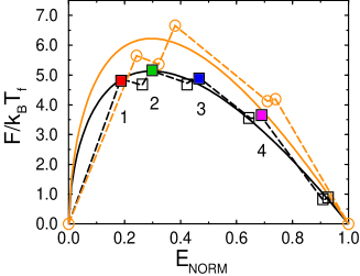
FIG. 1.: (color) The free energy at the stationary points along the folding route as a function of the normalized energy for the homogeneous (orange,$\circ$) and inhomogeneous (black,$\Box$) models. For an ensemble with average energy $E$, $E_{NORM}=(E-E_{G})/(E_{N}-E_{G})$, where $E_{N}$ and $E_{G}$ are the energies of the native state and globule state, respectively. $f_{{\rm cap}}$ (described in the text) is also shown as the solid line with $\gamma=$ 35(42) $k_{B}T_{f}$ for the heterogeneous(homogeneous) model.

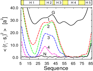
FIG. 2.: (color) The temperature factors (i.e., mean square fluctuations relative to the average position of $i^{th}$ monomer, ${\bf s}_{i}$) plotted as a function of sequence number for the heterogeneous model at the stationary points shown in Fig.1. The bar at the top indicates the helical secondary structure (H1-H5).

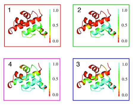
FIG. 3.: (color) The 3D native structure of $\lambda$-repressor colored according to the normalized energy of each site, $(e_{i}-e_{i}^{G})/(e_{i}^{N}-e_{i}^{G})$ with $e_{i}=\sum_{j}^{(N)}\epsilon_{ij}\langle u(r_{ij})\rangle_{0}$, evaluated at each saddle-point (clockwise from upper left). $e_{i}^{N}$ and $e_{i}^{G}$ are the energies of the $i^{th}$ site in the native state and globule state, respectively.

REFERENCES

- [1] P. E. Leopold, M. Montal, and J. N. Onuchic, Proc. Natl. Acad. Sci. U. S. A. 89, 8721 (1992); J. D. Bryngelson, J. N. Onuchic, N. D. Socci, and P. G. Wolynes, Proteins: Structure, Function and Genetics 21, 167 (1995).
- [2] W. A. Eaton et al., Curr. Opin. Struct. Biol. 7, 10 (1997).
- [3] A. R. Fersht, A. Matouschek, and L. Serrano, J. Mol. Biol. 224, 771 (1992).
- [4] S. S. Plotkin, J. Wang, and P. G. Wolynes, J. Chem. Phys. 106, 2932 (1997); J. N. Onuchic, N. D. Socci, Z. A. Luthey-Schulten, and P. G. Wolynes, Folding and Design 1, 441 (1996); Z. Guo, C. L. Brooks, and E. M. Boczko, Proc. Natl. Acad. Sci. U. S. A. 94, 10161 (1997).
- [5] M. Sasai and P. G. Wolynes, Phys. Rev. A 46, 7979 (1992); S. Takada and P. G. Wolynes, Phys. Rev. E 55, 4562 (1997); S. Takada and P. G. Wolynes, J. Chem. Phys. 107, 9585 (1997);
- [6] M. Bixon and R. Zwanzig, J. Chem. Phys. 68, 1896 (1978).
- [7] C. R. Cantor and P. R. Schimmel, Biophysical Chemistry (W. H. Freeman and Co., New York, 1980), Vol. 3, p. 1013.
- [8] J. D. Bryngelson and P. G. Wolynes, Proc. Natl. Acad. Sci. U. S. A. 84, 7524 (1987).
- [9] N. Gō, Annu. Rev. Biophys. Bioeng. 12, 183 (1983).
- [10] V. Pande and D. S. Rokhsar, Nature Struct. Biol. , (submitted).
- [11] S. F. Edwards and M. Muthukumar, J. Chem. Phys. 89, 2435 (1988); J. D. Honeycutt and D. Thirumalai, J. Chem. Phys. 90, 4542 (1989).
- [12] M. Mézard and G. Parisi, J. Phys. I(France) 1, 809 (1991); T. Garel and H. Orland, Phys. Rev. B 55, 226 (1997).
- [13] A. Moskalenko, Y. A. Kuznetsov, and K. A. Dawson, Physica A 249, 353 (1998).
- [14] D. J. Wales, J. Chem. Phys. 101, 3750 (1994).
- [15] R. E. Burton et al., J. Mol. Biol. 263, 311 (1996).
- [16] R. E. Burton et al., Nature Struct. Biol. 4, 305 (1997).
- [17] L. J. Beamer and C. O. Pabo, J. Mol. Biol. 227, 177 (1992).
- [18] S. Miyazawa and R. L. Jernigan, J. Mol. Biol. 256, 623 (1996).
- [19] J. D. Bryngleson and P. G. Wolynes, Biopolymers 30, 177 (1990); A. V. Finkelstein and A. Y. Badretdinov, Folding and Design 2, 115 (1997); P. G. Wolynes, Proc. Natl. Acad. Sci. U. S. A. 94, 6170 (1997).
- [20] M. Silow and M. Oliveberg, J. Mol. Biol. 269, 611 (1997).
- [21] Villain, J. Phys. I(France) 46, 1843 (1985).