PHYSICAL REVIEW B        VOLUME 59, NUMBER 1 1 JANUARY 1999-I, 443-456 Classical spin liquid: Exact solution for the infinite-component antiferromagnetic model on the $\textstyle kagom\mathaccent 19{e}$ lattice

I Introduction

Classical antiferromagnets on kagomé and pyrochlore lattices built of corner-sharing triangles and tetrahedra, respectively, are examples of frustrated systems which cannot order because of the high degeneracy of their ground state [4] and ensuing large fluctuations. Monte Carlo (MC) simulations for kagomé [5] and pyrochlore [6] lattices with the nearest-neighbor (nn) interaction $J$ show a smooth temperature dependence of the heat capacity, $C(T)$, in the entire temperature range. The spin correlation functions (CF’s) of both models show only weak short-range order at $T\,\raisebox{1.50696pt}{$<$}\raisebox{-2.79857pt}{$\sim$}\,J$ and decay at distances of the order of several lattice spacings $a_{0}$. This is in a striking contrast to the long-range order in common three-dimensional magnets and the extended short-range order [strong correlation at the distances $r\,\raisebox{1.50696pt}{$<$}\raisebox{-2.79857pt}{$\sim$}\,\xi_{c}\propto\exp(T^{*}/T)$ with $T^{*}\sim J$] in common two-dimensional magnets.

Spin-wave calculations starting from one of the ordered states of the kagomé lattice [7] (see, also, Ref. [8] for the quantum case) yield a twofold degenerate Goldstone mode, as well as a zero-energy mode for all values of the wave vector $q$ in the Brillouin zone, the latter reflecting the instability of the ground states. Mean-field approximation (MFA) at elevated temperatures for both kagomé and pyrochlore lattices [4] reflects the same behavior. The maximal eigenvalues of the Fourier-transformed exchange interaction matrix are $q$ independent for both models (and twofold degenerate for pyrochlore). Thus the system cannot choose the ordering wave vector at the mean-field transition temperature, $T_{c}^{\rm MFA}$, which in fact shows that there is no phase transition at this temperature because of fluctuations. This results in the smooth temperature dependence of the thermodynamic quantities [5, 6] and in the diffuse magnetic neutron scattering. [9]

The degeneracy of the ground state of these models can be lifted by small perturbations, such as dipole-dipole interactions, lattice distortions, next-nearest-neighbor (nnn) or long-range interactions, and quantum effects. This may be a reason why pyrochlore antiferromagnets usually freeze into a spin-glass state with lowering temperature. [10, 11] Theoretically, the most transparent way to lift the degeneracy is to include nnn interactions in the Hamiltonian. [4] Experiment and MC simulations on pyrochlores [12] show ordering with an unusual critical behavior ($\beta\approx 0.18$) in this case. According to the spin-wave results of Ref. [13] for the kagomé lattice, at low temperatures dipole-dipole interactions favor the planar ${\bf q}=0$ phase which is characterized by the same ordering pattern in each of the elementary triangles.

A more subtle mechanism for lifting the degeneracy and selection of definite ordering patterns is the nonlinear interaction of spin waves for classical systems at very low temperatures, typically $T\,\raisebox{1.50696pt}{$<$}\raisebox{-2.79857pt}{$\sim$}\,0.01J$. For the kagomé lattice, nonlinear effects (thermal fluctuations) favor the coplanar spin configuration with the $\sqrt{3}\times\sqrt{3}$ short-range order in the case of the Heisenberg model, $D=3$, as was suggested by the results of MC simulations [5, 14, 15] and high-temperature series expansions. [7] Extension of the $\sqrt{3}\times\sqrt{3}$ short-range order into the true long-range order in the limit $T\to 0$ is, however, hampered by formation of chiral domain walls which cost no energy but provide a gain in entropy at low concentrations. [15] The configuration selection at low temperatures only occurs if the number of spin components $D$ is low enough. So, the early MC simulations of Ref.[14] for the kagomé antiferromagnet showed selection of a coplanar state for $D=3$, but no such selection for $D\geq 4$. For the pyrochlore lattice, early simulations showed the selection of the collinear spin ordering for the Heisenberg model at low temperatures, [12] although according to the recent results of Ref. [16] this happens only for the plane rotator model, $D=2$, and not for higher spin dimensionalities. The above results are in accord with general criterion for selection of ordered states as a function of spin and space dimensions for corner sharing objects, which was formulated in Ref. [16]. Quantum fluctuations were shown to stabilize the $\sqrt{3}\times\sqrt{3}$ phase for $S\gg 1$, [17] but they should destroy ordering for low spin values $S$. [8, 18, 19, 20] One of the possible mechanisms for that is tunneling of the weatherwane (hard hexagon) mode in the $\sqrt{3}\times\sqrt{3}$ structure. [21]

It should be stressed, however, that the subtle effects quoted above can be easily overwhelmed by more trivial and robust ones, and they are much easier to observe in simulations than in experiment. The first task of the theory is thus to describe the principal features of classical spin models on frustrating lattices, as, e.g., a smooth variation of the thermodynamic quantities in the whole temperature range. The simplest approach, the MFA, is clearly inapplicable in this case, whereas the more powerful tools of the theory of critical phenomena, such as the renormalization group, seem to have not been yet applied to these lattices.

The “next simplest” approximation for classical spin systems, which follows the MFA, consists in generalizing the Heisenberg Hamiltonian for the $D$-component spin vectors: [22, 23]

$${\cal H}=-\mathchoice{{\hbox{\boldmath$\displaystyle\rm H\cdot$}}}{{\hbox{\boldmath$\textstyle\rm H\cdot$}}}{{\hbox{\boldmath$\scriptstyle\rm H\cdot$}}}{{\hbox{\boldmath$\scriptscriptstyle\rm H\cdot$}}}\sum_{r}{\bf s}_{r}-\frac{1}{2}\sum_{rr^{\prime}}J_{rr^{\prime}}{\bf s}_{r}\mathchoice{{\hbox{\boldmath$\displaystyle\cdot\rm s$}}}{{\hbox{\boldmath$\textstyle\cdot\rm s$}}}{{\hbox{\boldmath$\scriptstyle\cdot\rm s$}}}{{\hbox{\boldmath$\scriptscriptstyle\cdot\rm s$}}}_{r^{\prime}},\qquad|{\bf s}_{r}|=1$$ (1)

and taking the limit $D\to\infty$. In this limit the problem becomes exactly solvable for all lattice dimensionalities, $d$, and the partition function of the system coincides [24] with that of the spherical model. [25, 26] The $D=\infty$ model possesses, however, a number of important advantages with respect to the spherical one. (i) The $1/D$ expansion is possible, [27, 28, 29] including the case of low-dimensional systems. [30, 31] The calculations can be done conveniently in the framework of the diagram technique for classical spin systems. [32, 30, 33] (ii) Inclusion of anisotropic terms in Eq. (1) is possible, too, which allows us to describe ordering in low dimensions, including thin films [34] and domain walls. [35] (iii) In spatially inhomogeneous cases the $D=\infty$ model yields physically correct results, in contrast to the spherical model failing on the global spin constraint. [36] (iv) Below the Curie temperature $T_{c}$ or in a magnetic field, the $D=\infty$ model describes both transverse and longitudinal CF’s (Ref. [37]) that differ from each other, in contrast to the single CF in the spherical model.

The $D=\infty$ model properly accounts for the profound role played, especially in low dimensions, by the Goldstone or would be Goldstone modes. At the same time, the less significant effects of the critical fluctuation coupling leading, e.g., to the quantitatively different nonclassical critical indices, die out in the limit $D\to\infty$. Thus this model is a relatively simple yet a powerful tool for classical spin systems. It should not be mixed up with the $N$-flavor generalization of the quantum $S=1/2$ model [38] in the limit $N\to\infty$, including its $1/N$ expansion. [18, 39] The $N$-component nonlinear $\sigma$-model (see, e.g., Refs. [40], as well as Ref. [41], and [42] for the $1/N$ expansion) is a quantum extension of Eq. (1) in the long-wavelength region at low temperatures. Effective free energies for the $n$-component order parameter appear, instead of Eq. (1), in conventional theories of critical phenomena. Using them for the $1/n$ expansion (see, e.g., Ref. [43]) is a matter of taste. While yielding the same results for the critical indices as the lattice-based $1/D$ expansion, [27, 28, 29] it misses the absolute values of the nonuniversal quantities. The same comment also applies to the spatially inhomogeneous systems in the limit $D=n=\infty$, such as semi-infinite ferromagnets (cf. Refs. [44] and [45]).

In this article the solution for the isotropic antiferromagnetic infinite-component spin-vector model on the kagomé lattice will be given. The qualitatively similar results for the pyrochlore lattice will be presented in a subsequent communication. As long as the system studied is homogeneous, isotropic, and in zero magnetic field, the standard spherical model [25, 26] can be applied, too. Such an approach for nonordering frustrated three-dimensional systems has been advocated in Ref. [46]. We prefer, however, to use the more general framework.

The rest of this article is organized as follows. In Sec. II the structure of the kagomé lattice and its collective spin variables are described. In Sec. III the formalism of the $D=\infty$ model is tailored for the kagomé lattice. The diagrams of the classical spin diagram technique that do not disappear in the limit $D\to\infty$ are summed up. The general analytical expressions for the thermodynamic functions and spin CF’s for all temperatures are obtained. In Sec. IV the thermodynamic quantities of the kagomé antiferromagnet (AFM) are calculated and compared with MC simulation results in the whole temperature range. In Sec. V the real space correlation functions are computed. In Sec. VI the neutron scattering cross section is worked out. In Sec. VII possible improvements of the present approach, such as the $1/D$ expansion, are discussed.

II Lattice structure and the Hamiltonian

\begin{picture}(11.0,7.0)\centerline{\hbox{\psfig{angle=0,width=227.62204pt}}} \end{picture}

FIG. 1.: Structure of the kagomé lattice. The elementary triangles are labeled by the pairs of numbers $n_{u},n_{v}$ according to Eq. (2), and the sites on triangles (the sublattices) are labeled by $l=1,2,3$. The configuration shown corresponds to the coplanar $\sqrt{3}\times\sqrt{3}$ structure characterized by the ordering wave vector ${\bf q}_{\sqrt{3}}$ given by Eq. (7).

The kagomé lattice shown in Fig. 1 consists of corner-sharing triangles. Each node of the corresponding Bravais lattice (i.e., each elementary triangle in Fig. 1) is numbered by $i,j=1,\ldots,N$. Each site of the elementary triangle is labeled by the index $l=1,2,3$. It is convenient to use the dimensionless units in which the interatomic distance equals 1 and hence the lattice period equals 2. The triangles numbered by $i,j=1,\ldots,N$ can be obtained from each other by the translations

$${\bf r}_{j}^{l}={\bf r}_{i}^{l}+n_{u}2{\bf u}+n_{v}2{\bf v},$$ (2)

where ${\bf r}_{i}^{l}$ is the position of a site on the lattice, $n_{u}$ and $n_{v}$ are integers, $2{\bf u}$ and $2{\bf v}$ are the elementary translation vectors (lattice periods), and

$${\bf u}=(1,0),\qquad{\bf v}=(-1/2,\sqrt{3}/2).$$ (3)

One of the most symmetric phases of the kagomé AFM is the so-called $\sqrt{3}\times\sqrt{3}$ phase which is shown in Fig. 1. This coplanar phase can be described by the complex “spin” $\tilde{s}_{\bf r}\equiv s_{\bf r}^{x}+is_{\bf r}^{y}=\exp(i{\bf q}_{\sqrt{3}}\mathchoice{{\hbox{\boldmath$\displaystyle\rm\cdot r$}}}{{\hbox{\boldmath$\textstyle\rm\cdot r$}}}{{\hbox{\boldmath$\scriptstyle\rm\cdot r$}}}{{\hbox{\boldmath$\scriptscriptstyle\rm\cdot r$}}}+i\phi_{0})$, where the ordering wave vector ${\bf q}_{\sqrt{3}}$ can be written in three equivalent forms:

$${\bf q}_{\sqrt{3}}=-\frac{2\pi}{3}\times\left\{\begin{array}[]{l}{\bf u}\\ {\bf v}\\ {\bf w},\end{array}\right.$$ (7)

where ${\bf w}=(-1/2,-\sqrt{3}/2)$. In this phase spins rotate by $-240^{\circ}=120^{\circ}$ as ${\bf r}$ changes by the lattice period 2 in each of the directions ${\bf u}$, ${\bf v}$, and ${\bf w}$ making the angle $120^{\circ}$ with each other. Another realization of the $\sqrt{3}\times\sqrt{3}$ phase, in which spins rotate by $-120^{\circ}$, is described by ${\bf q}_{\sqrt{3}}$ with positive sign. In addition, the $\sqrt{3}\times\sqrt{3}$ phase can be described by appropriate combinations of different forms of ${\bf q}_{\sqrt{3}}$ given above.

To facilitate the diagram summation in the next section, it is convenient to put the Hamiltonian (1) into a diagonal form. First, one goes to the Fourier representation according to

$${\bf s}_{\bf q}^{l}=\sum_{i}{\bf s}_{i}^{l}e^{-i\mathchoice{{\hbox{\boldmath$\displaystyle\rm q\cdot r$}}}{{\hbox{\boldmath$\textstyle\rm q\cdot r$}}}{{\hbox{\boldmath$\scriptstyle\rm q\cdot r$}}}{{\hbox{\boldmath$\scriptscriptstyle\rm q\cdot r$}}}_{i}^{l}},\qquad{\bf s}_{i}^{l}=\frac{1}{N}\sum_{\bf q}{\bf s}_{\bf q}^{l}e^{i\mathchoice{{\hbox{\boldmath$\displaystyle\rm q\cdot r$}}}{{\hbox{\boldmath$\textstyle\rm q\cdot r$}}}{{\hbox{\boldmath$\scriptstyle\rm q\cdot r$}}}{{\hbox{\boldmath$\scriptscriptstyle\rm q\cdot r$}}}_{i}^{l}},$$ (8)

where the wave vector ${\bf q}$ belongs to the hexagonal Brillouin zone specified by the corners $(\pm\pi/3,\pm\pi/\sqrt{3})$ and $(\pm 2\pi/3,0)$ (see Fig. 2). The Fourier-transformed Hamiltonian reads

$${\cal H}=\frac{1}{2N}\sum_{ll^{\prime}\bf q}V_{\bf q}^{ll^{\prime}}{\bf s}_{\bf q}^{l}\mathchoice{{\hbox{\boldmath$\displaystyle\cdot\rm s$}}}{{\hbox{\boldmath$\textstyle\cdot\rm s$}}}{{\hbox{\boldmath$\scriptstyle\cdot\rm s$}}}{{\hbox{\boldmath$\scriptscriptstyle\cdot\rm s$}}}_{-{\bf q}}^{l^{\prime}},$$ (9)

where the interaction matrix is given by

$$\hat{V}_{\bf q}=2J\left(\begin{array}[]{ccc}0&a&b\\ a&0&c\\ b&c&0\end{array}\right),\qquad\begin{array}[]{l}a\equiv\cos({\bf u\cdot q})\\ b\equiv\cos({\bf v\cdot q})\\ c\equiv\cos({\bf w\cdot q}).\\ \end{array}$$ (10)

At the second stage, the Hamiltonian (9) is finally diagonalized to the form

$${\cal H}=-\frac{1}{2N}\sum_{n\bf q}\tilde{V}_{\bf q}^{n}\mathchoice{{\hbox{\boldmath$\displaystyle\sigma$}}}{{\hbox{\boldmath$\textstyle\sigma$}}}{{\hbox{\boldmath$\scriptstyle\sigma$}}}{{\hbox{\boldmath$\scriptscriptstyle\sigma$}}}_{\bf q}^{n}\mathchoice{{\hbox{\boldmath$\displaystyle\cdot\sigma$}}}{{\hbox{\boldmath$\textstyle\cdot\sigma$}}}{{\hbox{\boldmath$\scriptstyle\cdot\sigma$}}}{{\hbox{\boldmath$\scriptscriptstyle\cdot\sigma$}}}_{-\bf q}^{n},$$ (11)

where $\tilde{V}_{\bf q}^{n}=2J\nu_{n}({\bf q})$ are the eigenvalues of the matrix $V_{\bf q}^{ll^{\prime}}$ taken with the negative sign,

$$\nu_{1}=1,\qquad\nu_{2,3}=(\pm\sqrt{1+8abc}-1)/2.$$ (12)

The diagonalizing transformation has the explicit form

$$U_{nl}^{-1}({\bf q})V^{ll^{\prime}}_{\bf q}U_{l^{\prime}n^{\prime}}({\bf q})=\tilde{V}^{n}_{\bf q}\delta_{nn^{\prime}},$$ (13)

where the summation over the repeated indices is implied and $\hat{U}$ is the real unitary matrix, $\hat{U}^{-1}=\hat{U}^{T}$, i.e., $U_{nl}^{-1}=U_{ln}$. The columns of the matrix $\hat{U}$ are the three normalized eigenvectors $U_{n}=(U_{1n},U_{2n},U_{3n})$ of the interaction matrix $\hat{V}$:

$$U_{n}=(ac-b\nu_{n},\;ab-c\nu_{n},\;\nu_{n}^{2}-a^{2})/\sqrt{Q_{n}},$$ (14)

$$Q_{n}=(\nu_{n}^{2}-a^{2})^{2}+(ab-c\nu_{n})^{2}+(ac-b\nu_{n})^{2}.$$ (15)

The eigenvector $U_{1}$ corresponding to the dispersionless eigenvalue $\nu_{1}=1$ can be represented in the unnormalized form as

$$U_{1}=[\sin(\mathchoice{{\hbox{\boldmath$\displaystyle\rm w\cdot q$}}}{{\hbox{\boldmath$\textstyle\rm w\cdot q$}}}{{\hbox{\boldmath$\scriptstyle\rm w\cdot q$}}}{{\hbox{\boldmath$\scriptscriptstyle\rm w\cdot q$}}}),\;\sin(\mathchoice{{\hbox{\boldmath$\displaystyle\rm v\cdot q$}}}{{\hbox{\boldmath$\textstyle\rm v\cdot q$}}}{{\hbox{\boldmath$\scriptstyle\rm v\cdot q$}}}{{\hbox{\boldmath$\scriptscriptstyle\rm v\cdot q$}}}),\;\sin(\mathchoice{{\hbox{\boldmath$\displaystyle\rm u\cdot q$}}}{{\hbox{\boldmath$\textstyle\rm u\cdot q$}}}{{\hbox{\boldmath$\scriptstyle\rm u\cdot q$}}}{{\hbox{\boldmath$\scriptscriptstyle\rm u\cdot q$}}})].$$ (16)

The normalized eigenvectors satisfy the requirements of orthogonality and completeness, respectively,

$$U_{ln}({\bf q})U_{ln^{\prime}}({\bf q})=\delta_{nn^{\prime}},\qquad U_{ln}({\bf q})U_{l^{\prime}n}({\bf q})=\delta_{ll^{\prime}}.$$ (17)

The Fourier components of the spins ${\bf s}_{\bf q}^{l}$ and the collective spin variables $\mathchoice{{\hbox{\boldmath$\displaystyle\sigma$}}}{{\hbox{\boldmath$\textstyle\sigma$}}}{{\hbox{\boldmath$\scriptstyle\sigma$}}}{{\hbox{\boldmath$\scriptscriptstyle\sigma$}}}_{\bf q}^{n}$ are related by

$${\bf s}_{\bf q}^{l}=U_{ln}({\bf q})\mathchoice{{\hbox{\boldmath$\displaystyle\sigma$}}}{{\hbox{\boldmath$\textstyle\sigma$}}}{{\hbox{\boldmath$\scriptstyle\sigma$}}}{{\hbox{\boldmath$\scriptscriptstyle\sigma$}}}_{\bf q}^{n},\qquad\mathchoice{{\hbox{\boldmath$\displaystyle\sigma$}}}{{\hbox{\boldmath$\textstyle\sigma$}}}{{\hbox{\boldmath$\scriptstyle\sigma$}}}{{\hbox{\boldmath$\scriptscriptstyle\sigma$}}}_{\bf q}^{n}={\bf s}_{\bf q}^{l}U_{ln}({\bf q}).$$ (18)

\begin{picture}(11.0,8.0)\centerline{\hbox{\psfig{angle=0,width=256.0748pt}}} \end{picture}

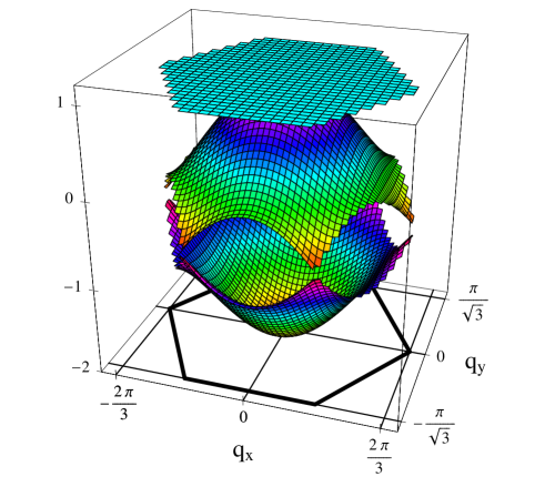
FIG. 2.: Reduced eigenvalues of the interaction matrix, $\nu_{n}({\bf q})=\tilde{V}_{\bf q}^{n}/(2J)$ of Eq. (11), plotted over the Brillouin zone.

The largest dispersionless eigenvalue $\nu_{1}$ of the interaction matrix [see Eq. (12)] manifests frustration in the system which precludes an extended short-range order even in the limit $T\to 0$. Independence of $\nu_{1}$ of ${\bf q}$ signals that 1/3 of all spin degrees of freedom are local and can rotate freely. The other two eigenvalues satisfy

$$\nu_{2}({\bf q})\cong 1-q^{2}/2,\qquad\nu_{3}({\bf q})\cong-2+q^{2}/2$$ (19)

at small wave vectors, $q^{2}\equiv q_{x}^{2}+q_{y}^{2}\ll 1$. The eigenvalue $\nu_{2}$ which becomes degenerate with $\nu_{1}$ in the limit $q\to 0$ is related, as we shall see below, to the usual would be Goldstone mode destroying the long-range order in low-dimensional magnets with a continuous symmetry. The eigenvalue $\nu_{3}$ is positioned, in the long-wavelength region, much lower than the first two, and it is tempting to call it the “optical” eigenvalue. In fact, however, the eigenvalues of the interaction matrix are not the same as the normal modes of the system that appear in the dynamics. Whereas $\nu_{1}$ gives rise to the zero-energy spin-wave branch corresponding to the absence of a restoring force for small deviations from one of degenerate ground states, $\nu_{2}$ and $\nu_{3}$ hybridize to the double-degenerate Goldstone mode with energy $\propto q$ at small wave vectors, as in conventional antiferromagnets. [8, 7] With increasing $q$ the eigenvalue $\nu_{2}$ decreases whereas $\nu_{3}$ increases; at the corners of the Brillouin zone they become degenerate: $\nu_{2}=\nu_{3}=-1/2$. The ${\bf q}$ dependences of the eigenvalues $\nu_{n}$ over the whole Brillouin zone is shown in Fig. 2.

In contrast to the smooth behavior of $\nu_{n}$, the diagonalizing matrix $\hat{U}$ composed of the eigenvectors $U_{n}$ [see Eq. (14)] has much more complicated structure as function of ${\bf q}$. This results in the intricate behavior of the spin CF’s and neutron-scattering cross sections at low temperatures, which will be considered in Sec. V. Here we only show the nonanalytic limiting form of $\hat{U}$ at small wave vectors,

$$\hat{U}_{\bf q}\cong\frac{1}{\sqrt{6}}\left(\begin{array}[]{ccc}-n_{x}-\sqrt{3}n_{y}&-n_{y}+\sqrt{3}n_{x}&\sqrt{2}\\ -n_{x}+\sqrt{3}n_{y}&-n_{y}-\sqrt{3}n_{x}&\sqrt{2}\\ 2n_{x}&2n_{y}&\sqrt{2}\end{array}\right),$$ (20)

where ${\bf n}\equiv{\bf q}/q$.

In the next section the equations describing spin correlation functions of the classical kagomé antiferromagnet in the large-$D$ limit will be obtained with the help of the classical spin diagram technique. The readers who are not interested in details can skip to Eq. (42) or directly to Sec. IV.

III Classical spin diagram technique and the large-$D$ limit

The exact equations for spin correlation functions in the limit $D\to\infty$, as well as the $1/D$ corrections, can be the most conveniently obtained with the help of the classical spin diagram technique. [32, 30, 33] A perturbative expansion of the thermal average of any quantity ${\cal A}$ characterizing a classical spin system (e.g., ${\cal A}=s_{zi}$ — the $z$ spin component on the lattice site $i$) can be obtained by rewriting Eq. (1) as ${\cal H}={\cal H}_{0}+{\cal H}_{\rm int}$, where ${\cal H}_{0}$ is, e.g., the mean-field Hamiltonian, and expanding the expression

$$\langle{\cal A}\rangle=\frac{1}{{\cal Z}}\int\prod_{j=1}^{N}d{\bf s}_{j}{\cal A}\exp(-\beta{\cal H}),\qquad|{\bf s}_{j}|=1,$$ (21)

where $\beta=1/T$, in powers of ${\cal H}_{\rm int}$. The integration in Eq. (21) is carried out with respect to the orientations of the $D$-dimensional unit vectors ${\bf s}_{j}$ on each of the lattice sites. Averages of various spin-vector components on various lattice sites with the Hamiltonian ${\cal H}_{0}$ can be expressed through spin cumulants, or semi-invariants, which will be considered below, in the following way:

$$\langle s_{\alpha i}\rangle_{0}=\Lambda_{\alpha},$$ (22)

$$\langle s_{\alpha i}s_{\beta j}\rangle_{0}=\Lambda_{\alpha\beta}\delta_{ij}+\Lambda_{\alpha}\Lambda_{\beta},$$ (23)

$$\langle s_{\alpha i}s_{\beta j}s_{\gamma k}\rangle_{0}=\Lambda_{\alpha\beta\gamma}\delta_{ijk}+\Lambda_{\alpha\beta}\Lambda_{\gamma}\delta_{ij}$$ (24)

$$\qquad\qquad\qquad+\,\Lambda_{\beta\gamma}\Lambda_{\alpha}\delta_{jk}+\Lambda_{\gamma\alpha}\Lambda_{\beta}\delta_{ki}+\Lambda_{\alpha}\Lambda_{\beta}\Lambda_{\gamma},$$ (25)

etc., where $\delta_{ij}$, $\delta_{ijk}$, etc., are the site Kronecker symbols equal to 1 for all site indices coinciding with each other and to zero in all other cases. For the one-site averages ($i=j=k=\ldots$) Eq. (22) reduces to the well-known representation of moments through semi-invariants, generalized for a multicomponent case. In the graphical language (see Fig. 3) the decomposition (22) corresponds to all possible groupings of small circles (spin components) into oval blocks (cumulant averages). The circles coming from ${\cal H}_{\rm int}$ (the “inner” circles) are connected pairwise by the wavy interaction lines representing $\beta J_{ij}$. In diagram expressions, summations over site indices $i$ and component indices $\alpha$ of inner circles are carried out. One should not take into account disconnected (unlinked) diagrams [i.e., those containing disconnected parts with no “outer” circles belonging to ${\cal A}$ in Eq. (21)], since these diagrams are compensated for by the expansion of the partition function ${\cal Z}$ in the denominator of Eq. (21). Consideration of combinatorial numbers shows that each diagram contains the factor $1/n_{s}$, where $n_{s}$ is the number of symmetry group elements of a diagram [see, e.g., the factor $1/2!$ in Eq. (37) below]. The symmetry operations do not concern outer circles, which serve as a distinguishable “root” to build up more complicated (e.g., renormalized) diagrams. For spatially homogeneous systems, it is more convenient to use the Fourier representation and to calculate integrals over the wave vectors in the Brillouin zone rather than lattice sums. As due to the Kronecker symbols in Eq. (22) lattice sums are subject to the constraint that the coordinates of the circles belonging to the same block coincide with each other, the sum of wave vectors coming to or going out of any block along interaction lines is zero. So, for our model the pair cumulant average of the Fourier components defined by Eq. (8) reads

$$\langle s_{\alpha\bf q}^{l}s_{\beta{\bf q}^{\prime}}^{l^{\prime}}\rangle_{0,\rm cum}=\Lambda_{\alpha\beta}N\delta_{{\bf q}^{\prime},-{\bf q}}\delta_{ll^{\prime}},$$ (26)

where $\delta_{ll^{\prime}}$ is the sublattice Kronecker symbol. The cumulant spin averages in Eq. (22) can be obtained by differentiating the generating function $\Lambda(\xi)$ over appropriate components of the dimensionless field $\mathchoice{{\hbox{\boldmath$\displaystyle\xi$}}}{{\hbox{\boldmath$\textstyle\xi$}}}{{\hbox{\boldmath$\scriptstyle\xi$}}}{{\hbox{\boldmath$\scriptscriptstyle\xi$}}}\equiv\beta{\bf H}$: [32]

$$\Lambda_{\alpha_{1}\alpha_{2}\ldots\alpha_{p}}(\mathchoice{{\hbox{\boldmath$\displaystyle\xi$}}}{{\hbox{\boldmath$\textstyle\xi$}}}{{\hbox{\boldmath$\scriptstyle\xi$}}}{{\hbox{\boldmath$\scriptscriptstyle\xi$}}})=\frac{\partial^{p}\Lambda(\xi)}{\partial\xi_{\alpha_{1}}\partial\xi_{\alpha_{2}}\ldots\partial\xi_{\alpha_{p}}},$$ (27)

$$\Lambda(\xi)=\ln{\cal Z}_{0}(\xi),$$ (28)

where $\xi\equiv|\mathchoice{{\hbox{\boldmath$\displaystyle\xi$}}}{{\hbox{\boldmath$\textstyle\xi$}}}{{\hbox{\boldmath$\scriptstyle\xi$}}}{{\hbox{\boldmath$\scriptscriptstyle\xi$}}}|$,

$${\cal Z}_{0}(\xi)={\rm const}\times\xi^{-(D/2-1)}I_{D/2-1}(\xi)$$ (29)

is the partition function of a $D$-component classical spin, and $I_{\nu}(\xi)$ is the modified Bessel function. For the two lowest-order cumulants the differentiation in Eq. (27) leads to the following expressions:

$$\Lambda_{\alpha}(\mathchoice{{\hbox{\boldmath$\displaystyle\xi$}}}{{\hbox{\boldmath$\textstyle\xi$}}}{{\hbox{\boldmath$\scriptstyle\xi$}}}{{\hbox{\boldmath$\scriptscriptstyle\xi$}}})=B(\xi)\,\xi_{\alpha}/\xi,$$ (30)

$$\Lambda_{\alpha\beta}(\mathchoice{{\hbox{\boldmath$\displaystyle\xi$}}}{{\hbox{\boldmath$\textstyle\xi$}}}{{\hbox{\boldmath$\scriptstyle\xi$}}}{{\hbox{\boldmath$\scriptscriptstyle\xi$}}})=\frac{B(\xi)}{\xi}\left(\delta_{\alpha\beta}-\frac{\xi_{\alpha}\xi_{\beta}}{\xi^{2}}\right)+B^{\prime}(\xi)\frac{\xi_{\alpha}\xi_{\beta}}{\xi^{2}}.$$ (31)

where $\delta_{\alpha\beta}$ is the Kronecker symbol for spin components,

$$B(\xi)=d\Lambda(\xi)/d\xi=I_{D/2}(\xi)/I_{D/2-1}(\xi)$$ (32)

is the Langevin function of $D$-component classical spins, and $B^{\prime}(\xi)=dB/d\xi$ (see the details in Ref. [33]). If ${\cal H}_{0}=0$, as is the case for our model in the absence of a magnetic field, the pair spin cumulant in Eq. (30) simplifies to the obvious form

$$\Lambda_{\alpha\beta}(0)=\Lambda_{\alpha\alpha}(0)\delta_{\alpha\beta},\qquad\Lambda_{\alpha\alpha}(0)=1/D.$$ (33)

\begin{picture}(11.0,4.0)\centerline{\hbox{\psfig{angle=0,width=455.24408pt}}} \end{picture}

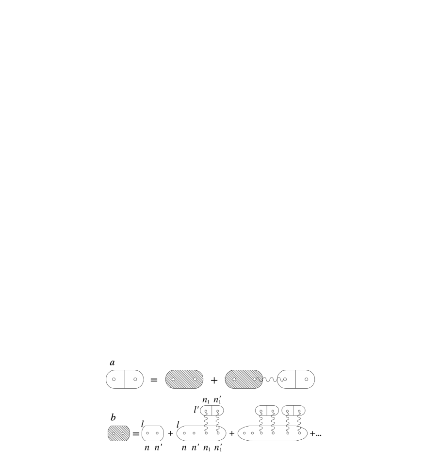
FIG. 3.: Self-consistent Gaussian approximation (SCGA) for classical spin systems in the nonordered state. ($a$) the Dyson equation for the spin correlation function; ($b$) the block summation for the renormalized pair cumulant spin averages.

As was shown in Ref. [32] (see also Ref. [30]) the limit $D\to\infty$ for the spin-vector model is completely described by the self-consistent Gaussian approximation (SCGA), since all diagrams not accounted for by the SCGA vanish in this limit. The SCGA consists in taking into account pair correlations of the molecular field acting on a given spin from its neighbors, which implies a Gaussian statistics of molecular field fluctuations. The appropriate diagram sequence for the nonordered state, $\langle s_{z}\rangle=0$, is represented in Fig. 3. Its analytical form for the square lattice model is given in Ref. [30]. In a magnetic field or below $T_{c}$ in the ordering models the average spin polarization $\langle s_{z}\rangle\neq 0$ appears. The additional diagrams and corresponding analytical expressions can be found in Refs. [32, 33], and [31]. The SCGA equations in the spatially inhomogeneous case and their large-$D$ limit have been derived (and applied to domain walls) in Ref. [35].

In all cases above, the SCGA equations have been written for diagonal Hamiltonians describing the simplest one-sublattice magnets. For nondiagonal Hamiltonians, such as Eq. (9), the matrix interaction lines, here $-\beta V_{\bf q}^{ll^{\prime}}$, complicate the formalism. Simplification can be achieved by using the diagonalized Hamiltonian, for our model, Eq. (11). For the latter, however, the $\sigma$ counterparts of the one-site cumulant averages do not have a transparent meaning anymore since $\sigma$ is a combination of spins on different sites and sublattices. Thus the $\sigma$ cumulants should be specially worked out as follows. The pair $\sigma$ cumulant (which is in our model explicitly diagonal in the spin-component indices $\alpha,\beta$) can be rewritten in terms of the initial spin variables as

$$\langle\sigma_{\alpha\bf q}^{n}\sigma_{\alpha{\bf q}^{\prime}}^{n^{\prime}}\rangle_{0,\rm cum}=U_{ln}({\bf q})U_{l^{\prime}n^{\prime}}({\bf q}^{\prime})\langle s_{\alpha\bf q}^{l}s_{\alpha{\bf q}^{\prime}}^{l^{\prime}}\rangle_{0,\rm cum}.$$ (34)

With the use of Eq. (26) and the first of the relations (17), this can be simplified to the final form

$$\langle\sigma_{\alpha\bf q}^{n}\sigma_{\alpha{\bf q}^{\prime}}^{n^{\prime}}\rangle_{0,\rm cum}=\Lambda_{\alpha\alpha}N\delta_{{\bf q}^{\prime},-{\bf q}}\delta_{nn^{\prime}}.$$ (35)

Now, with the help of the results just obtained, the second diagram in the sum in Fig. 3$b$ can be written in the analytical form

$$A_{2}=U_{ln}({\bf q})U_{ln^{\prime}}({\bf q})\Lambda_{\alpha\alpha\beta\beta}L_{\beta l},$$ (36)

where the summation over the spin-component index $\beta$ is implied and the quantity $L_{\beta l}$ in the lowest (the second) order of the perturbation theory is given by

$$L_{\beta l}^{(2)}=\frac{1}{2!}\Lambda_{\beta\beta}\frac{1}{N}\sum_{l^{\prime}\bf p}\sum_{n_{1}}U_{ln_{1}}({\bf p})U_{l^{\prime}n_{1}}({\bf p})\beta\tilde{V}_{\bf p}^{n_{1}}$$ (37)

$$\qquad{}\times\sum_{n^{\prime}_{1}}U_{ln^{\prime}_{1}}({\bf p})U_{l^{\prime}n^{\prime}_{1}}({\bf p})\beta\tilde{V}_{\bf p}^{n^{\prime}_{1}}.$$ (38)

Here $\beta=1/T$ in front of $\tilde{V}$ cannot be confused with the spin component index $\beta$. This expression can be simplified in two ways. First, one can perform the sum over the index $l^{\prime}$ and use the first of Eqs. (17), which leads to

$$L_{\beta l}^{(2)}=\frac{1}{2!}\Lambda_{\beta\beta}\frac{1}{N}\sum_{n_{1}\bf p}(\beta\tilde{V}_{\bf p}^{n_{1}})^{2}U_{ln_{1}}^{2}({\bf p}).$$ (39)

Second, inverting the transformation (13) one can write

$$L_{\beta l}^{(2)}=\frac{1}{2!}\Lambda_{\beta\beta}\frac{1}{N}\sum_{l^{\prime}\bf p}(\beta V_{\bf p}^{ll^{\prime}})^{2}.$$ (40)

Taking into account the explicit form of $V_{\bf p}^{ll^{\prime}}$ given by Eq. (10), one can see that after the integration over the wave vector ${\bf p}$ expression (40) becomes independent of the sublattice index $l$. After this observation one can symmetrize Eq. (39) with respect to $l$. This leads to the vanishing of the diagonalization matrix by virtue of the first of Eqs. (17) and to the appearance of the factor 1/3. Now the summation over $l$ in Eq. (36) simplifies, and the diagonalization matrices convert, again, to $\delta_{nn^{\prime}}$. The result in the second order of the perturbation theory has the form

$$A_{2}=\Lambda_{\alpha\alpha\beta\beta}L_{\beta}^{(2)},\qquad L_{\beta}^{(2)}=\frac{\Lambda_{\beta\beta}}{3\cdot 2!}\frac{1}{N}\sum_{n_{1}\bf p}(\beta\tilde{V}_{\bf p}^{n_{1}})^{2}$$ (41)

($\delta_{nn^{\prime}}$ has been omitted) and it is independent of the eigenvalue index $n$ and of the wave vector ${\bf q}$.

The mechanism of the simplification of diagram expressions demonstrated above can be shown to work for whatever complicated diagrams. In all cases oval blocks represent cumulant spin averages $\Lambda_{\alpha_{1}\alpha_{2}\ldots\alpha_{p}}$, as in the original, nondiagonalized, version of the classical spin diagram technique. In all the elements connected to a given block summation over the eigenvalue indices $n$ is carried out. The diagonalizing matrix $\hat{U}$ disappears completely if correlation functions for the $\sigma$ variables,

$$\sigma^{n}({\bf q})=\frac{D}{N}\langle\sigma_{\alpha\bf q}^{n}\sigma_{\alpha,{-\bf q}}^{n}\rangle=\frac{1}{N}\langle\mathchoice{{\hbox{\boldmath$\displaystyle\sigma$}}}{{\hbox{\boldmath$\textstyle\sigma$}}}{{\hbox{\boldmath$\scriptstyle\sigma$}}}{{\hbox{\boldmath$\scriptscriptstyle\sigma$}}}_{\bf q}^{n}\mathchoice{{\hbox{\boldmath$\displaystyle\sigma$}}}{{\hbox{\boldmath$\textstyle\sigma$}}}{{\hbox{\boldmath$\scriptstyle\sigma$}}}{{\hbox{\boldmath$\scriptscriptstyle\sigma$}}}_{-\bf q}^{n}\rangle,$$ (42)

are considered. After the calculation of the latter the true spin CF’s can be found from the formula

$$s^{ll^{\prime}}({\bf q})=U_{ln}({\bf q})U_{l^{\prime}n}({\bf q})\sigma^{n}({\bf q})$$ (43)

following from Eq. (18). Note that $\sigma^{n}({\bf q})$ are eigenvalues of the correlation matrix $s^{ll^{\prime}}({\bf q})$ and they describe independent linear responses to appropriate wave-vector-dependent fields. As can be seen from Eq. (43), the eigenvectors describing the “normal modes” of the susceptibility are those of the interaction matrix $V^{ll^{\prime}}_{\bf q}$ in Eq. (9).

The analytical expression for the $\sigma$ CF in the SCGA, which satisfies the Dyson equation shown in Fig. 3$a$, has the Ornstein-Zernike form

$$\sigma^{n}({\bf q})=\frac{D\tilde{\Lambda}_{\alpha\alpha}}{1-\tilde{\Lambda}_{\alpha\alpha}\beta\tilde{V}_{\bf q}^{n}}.$$ (44)

This expression differs from that obtained by Reimers on the mean-field basis [9] by the replacement of the bare cumulant $\Lambda_{\alpha\alpha}=1/D$ by its renormalized value $\tilde{\Lambda}_{\alpha\alpha}$ determined by the diagram series Fig. 3$b$. The summation of these diagrams is documented in the most detailed way by Eqs. (3.16)–(3.19) of Ref. [33]. The result for $\tilde{\Lambda}_{\alpha\alpha}$ is given by the second line of Eq. (30) averaged over the Gaussian fluctuations of all components of the molecular field $\textstyle\xi$ with the dispersion defined by the quantity $L_{\alpha}$. In our model, fluctuations of different components of $\textstyle\xi$ are independent from each other and of the same dispersion, $L_{\alpha}=L$. Thus the quantity $\tilde{\Lambda}_{\alpha\beta}$ is diagonal and independent of $\alpha$. In the large-$D$ limit the multiple Gaussian integral determining $\tilde{\Lambda}_{\alpha\alpha}$ is dominated by the stationary point and the result simplifies to [30]

$$\tilde{\Lambda}_{\alpha\alpha}=\frac{2}{D}\frac{1}{1+\sqrt{1+8L/D}}.$$ (45)

Here the dispersion $L$ corresponding to the diagram series in Fig. 3 is given by the formula

$$L=\frac{\tilde{\Lambda}_{\alpha\alpha}}{3\cdot 2!}\sum_{n}v_{0}\!\!\!\int\!\!\!\frac{d{\bf q}}{(2\pi)^{d}}\frac{(\beta\tilde{V}_{\bf q}^{n})^{2}}{1-\tilde{\Lambda}_{\alpha\alpha}\beta\tilde{V}_{\bf q}^{n}}$$ (46)

generalizing Eq. (41). Here, the summation $(1/N)\sum_{\bf q}\ldots$ is replaced by the integration over the Brillouin zone, $v_{0}$ is the unit-cell volume, and $d$ is the spatial dimensionality. For the kagomé lattice we have $v_{0}=2\sqrt{3}$ and $d=2$. The expression for $L$ can be simplified to

$$L=\frac{\bar{P}-1}{2\tilde{\Lambda}_{\alpha\alpha}},\qquad\bar{P}\equiv\frac{1}{3}\sum_{n}P_{n},$$ (47)

where $P_{n}$ is the lattice Green function associated with the eigenvalue $n$:

$$P_{n}=v_{0}\!\!\!\int\!\!\!\frac{d{\bf q}}{(2\pi)^{d}}\frac{1}{1-\tilde{\Lambda}_{\alpha\alpha}\beta\tilde{V}_{\bf q}^{n}}.$$ (48)

Now one can eliminate $L$ from Eqs. (45) and (47), which yields the basic equation of the large-$D$ model,

$$D\tilde{\Lambda}_{\alpha\alpha}\bar{P}=1.$$ (49)

This nonlinear equation determining $\tilde{\Lambda}_{\alpha\alpha}$ as a function of temperature differs from those considered earlier [32, 30, 31, 33] by a more complicated form of $\bar{P}$ reflecting the lattice structure. The form of this equation is similar to that appearing in the theory of the usual spherical model. [25, 26] The meanings of both equations are, however, different. Whereas in the standard spherical model a similar equation account for the pretty unphysical global spin constraint, Eq. (49) here is, in fact, the normalization condition $\langle{\bf s}_{\bf r}^{2}\rangle=1$ for the spin vectors on each of the lattice sites ${\bf r}$ [see Eq. (21)]. Indeed, calculating the spin autocorrelation function in the form symmetrized over sublattices with the help of Eqs. (43), (17), and (44), one obtains

$$\langle{\bf s}_{\bf r}^{2}\rangle=v_{0}\!\!\!\int\!\!\!\frac{d{\bf q}}{(2\pi)^{d}}\frac{1}{3}\sum_{l}s^{ll}({\bf q})$$ (50)

$$\qquad{}=v_{0}\!\!\!\int\!\!\!\frac{d{\bf q}}{(2\pi)^{d}}\frac{1}{3}\sum_{n}\sigma^{n}({\bf q})=D\tilde{\Lambda}_{\alpha\alpha}\bar{P}.$$ (51)

That is, the spin-normalization condition is automatically satisfied in our theory by virtue of Eq. (49). After $\tilde{\Lambda}_{\alpha\alpha}$ has been found from this equation, the spin CF’s are readily given by Eqs. (44) and (43).

To avoid possible confusion, we should mention that in the paper of Reimers, Ref. [9], where Eq. (44) with the bare cumulant $\Lambda_{\alpha\alpha}=1/D$ has been obtained, the theoretical approach has been called the “Gaussian approximation (GA)”. This term taken from the conventional theory of phase transitions based on the Landau free-energy functional implies that the Gaussian fluctuations of the order parameter are considered. In the microscopic language, this merely means calculating correlation functions of fluctuating spins after applying the MFA. Such an approach is known to be inconsistent, since correlations are taken into account after they had been neglected. As a result, for the kagomé lattice one obtains a phase transition at the temperature $T_{c}=T_{c}^{\rm MFA}=2J/D$ but immediately finds that the approach breaks down below $T_{c}$ because of the infinitely strong fluctuations. In contrast to this MFA-based approach, the self-consistent Gaussian approximation used here allows, additionally, to the Gaussian fluctuations of the molecular field, which renormalize $\Lambda_{\alpha\alpha}$ and lead to the absence of a phase transition for this class of systems. The SCGA is, in a sense, a “double-Gaussian” approximation: The diagram series in Fig. 3$a$ allows for the Gaussian fluctuations of the order parameter, whereas that in Fig. 3$b$ describes Gaussian fluctuations of the molecular field.

To close this section, let us work out the expressions for the energy and the susceptibility of the kagomé antiferromagnet. For the energy of the whole system, using Eqs. (11) and (42), as well as the equivalence of all spin components, one obtains

$$U_{\rm tot}=\langle{\cal H}\rangle=-\frac{N}{2}\sum_{n}v_{0}\!\!\!\int\!\!\!\frac{d{\bf q}}{(2\pi)^{d}}\tilde{V}_{\bf q}^{n}\sigma^{n}({\bf q}).$$ (52)

To obtain the energy per spin $U$, one should divide this expression by $3N$. With the use of Eq. (44), the latter can be expressed through the lattice Green’s function $\bar{P}$ of Eq. (47); then with the help of Eq. (49) it can be put into the final form

$$U=\frac{T}{2}\left(D-\frac{1}{\tilde{\Lambda}_{\alpha\alpha}}\right).$$ (53)

The susceptibility per spin symmetrized over sublattices can be expressed through the spin CF’s as

$$\chi_{\bf q}=\frac{1}{3DT}\sum_{ll^{\prime}}s^{ll^{\prime}}({\bf q}).$$ (54)

With the use of Eq. (43) this can be rewritten in the form

$$\chi_{\bf q}=\frac{1}{3DT}\sum_{n}W_{n}^{2}({\bf q})\sigma^{n}({\bf q}),\qquad W_{n}({\bf q})\equiv\sum_{l}U_{ln}({\bf q}),$$ (55)

where the diagonalized CF’s are given by Eq. (44). From Eq. (20) it follows that in the limit ${\bf q}\to 0$ one has $W_{1}=W_{2}=0$ and $W_{3}=\sqrt{3}$. Thus the homogeneous susceptibility $\chi\equiv\chi_{0}$ simplifies to

$$\chi=\frac{1}{DT}\sigma^{3}(0).$$ (56)

As we shall see in the next section, disappearance of the terms with $n=1$ and 2 from this formula ensures the nondivergence of the homogeneous susceptibility of the kagomé antiferromagnet in the limit $T\to 0$. The situation for ${\bf q}\neq 0$ is much more intricate and it will be considered below in relation to the neutron-scattering cross section.

IV Thermodynamics of the kagomé antiferromagnet

To put the results obtained above into the form explicitly well behaved in the large-$D$ limit and allowing a direct comparison with the results obtained by other methods for systems with finite values of $D$, it is convenient to use the mean-field transition temperature $T_{c}^{\rm MFA}=2J/D$ as the energy scale. With this choice, one can introduce the reduced temperature $\theta$ and the so-called gap parameter $G$ according to

$$\theta\equiv\frac{T}{T_{c}^{\rm MFA}},\qquad G\equiv\frac{D}{\theta}\tilde{\Lambda}_{\alpha\alpha}.$$ (57)

In these terms, Eq. (49) rewrites as

$$\theta G\bar{P}(G)=1$$ (58)

and determines $G$ as function of $\theta$. Here $\bar{P}(G)$ is defined by Eq. (47), where

$$P_{n}=v_{0}\!\!\!\int\!\!\!\frac{d{\bf q}}{(2\pi)^{d}}\frac{1}{1-G\nu_{n}({\bf q})},\qquad P_{1}=\frac{1}{1-G},$$ (59)

and the reduced eigenvalues $\nu_{n}({\bf q})$ are given by Eq. (12). The $\sigma$ CF’s of Eq. (44), which are proportional to the integrands of $P_{n}$, can be rewritten in the form

$$\sigma^{n}({\bf q})=\frac{\theta G}{1-G\nu_{n}({\bf q})}.$$ (60)

Further, it is convenient to consider the reduced energy per spin defined by

$$\tilde{U}\equiv U/|U_{0}|,\qquad U_{0}=-J,$$ (61)

where $U_{0}$ is the energy per spin at zero temperature. With the help of Eq. (53) $\tilde{U}$ can be written as

$$\tilde{U}=\theta-1/G.$$ (62)

The homogeneous susceptibility $\chi$ of Eq. (56) can be rewritten with the help of Eq. (19) in the reduced form

$$\tilde{\chi}\equiv 2J\chi=\frac{G}{1+2G}.$$ (63)

The sense of calling $G$ the “gap parameter” is clear from Eq. (60). If $G=1$, then the gap in correlation functions closes: $\sigma^{1}$ turns to infinity, and $\sigma^{2}$ diverges at $q\to 0$. For nonordering models, it happens only in the limit $\theta\to 0$, however. The solution of Eq. (58) satisfies $G\leq 1$ and goes to zero at high temperatures. If $\theta\ll 1$, the function $\bar{P}$ is dominated by $P_{1}=1/(1-G)$, whereas $P_{3}$ remains of order unity and $P_{2}$ diverges only logarithmically, as in usual two-dimensional systems: $P_{2}\cong(\sqrt{3}/\pi)\ln[c/(1-G)]$, $c\sim 1$. The ensuing asymptotic form of the gap parameter at low temperatures reads

$$G\cong 1-\frac{\theta}{3}-\left(\frac{\theta}{3}\right)^{2}\frac{\sqrt{3}}{\pi}\ln\frac{3c}{\theta},\qquad\theta\ll 1.$$ (64)

At high temperatures, Eq. (58) requires small values of $G$. Here, the limiting form of $\bar{P}$ can be shown to be $\bar{P}\cong 1+G^{2}$. The corresponding asymptote of $G$ has the form

$$G\cong\frac{1}{\theta}\left(1-\frac{1}{\theta^{2}}\right),\qquad\theta\gg 1.$$ (65)

The numerically calculated temperature dependence of $G$ is shown in Fig. 4. Note that in the MFA one has $G=1/\theta$ which attains the value 1 at $\theta=1$.

\begin{picture}(11.0,7.0)\centerline{\hbox{\psfig{angle=-90,width=341.43306pt}}} \end{picture}

FIG. 4.: Temperature dependence of the gap parameter $G$ for the kagomé antiferromagnet.

\begin{picture}(11.0,7.0)\centerline{\hbox{\psfig{angle=-90,width=341.43306pt}}} \end{picture}

FIG. 5.: Temperature dependence of the reduced energy of the kagomé antiferromagnet.

\begin{picture}(11.0,7.0)\centerline{\hbox{\psfig{angle=-90,width=341.43306pt}}} \end{picture}

FIG. 6.: Temperature dependence of the heat capacity of the kagomé antiferromagnet. The MC results of Ref. [5] for the Heisenberg model ($D=3$) are represented by circles.

\begin{picture}(11.0,7.0)\centerline{\hbox{\psfig{angle=-90,width=341.43306pt}}} \end{picture}

FIG. 7.: Temperature dependence of the reduced uniform susceptibility of the kagomé antiferromagnet. The MC results of Ref. [15] for the Heisenberg model ($D=3$) are represented by circles.

The temperature dependence of the reduced energy of Eq. (62) is shown in Fig. 5. Its asymptotic forms following from Eqs. (64) and (65) are given by

$$\tilde{U}\cong\left\{\begin{array}[]{ll}-1/\theta,&\theta\gg 1\\ -1+(2/3)\theta,&\theta\ll 1.\end{array}\right.$$ (66)

This implies the reduced heat capacity $\tilde{C}=d\tilde{U}/d\theta$ is equal to 2/3 at low temperatures, in contrast to $\tilde{C}=1$ for usual two-dimensional lattices in the same approximation. The latter result is solely due to the term linear in $\theta$ in Eq. (62), whereas $G$ only exponentially deviates from 1 at low temperatures. For the kagomé lattice, there is a linear in $\theta$ contribution to the gap parameter $G$ of Eq. (64), which leads to $\tilde{C}=2/3$. This reflects the fact that one of three modes in the kagomé lattice [see Eq. (11)] is dispersionless, and hence 1/3 of all spin degrees of freedom in the system are local and free, making no contribution to the heat capacity.

The reduced variables introduced at the beginning of this section are very convenient for the comparison of the results for $D=\infty$ with those for finite values of $D$, which are obtained by other methods. The expected discrepancies are of order $1/D$ which is not too much for $D=3$. (Note that the $D=\infty$ approximation can be improved by the $1/D$ expansion. [30, 31]) To compare with the MC simulation data of Ref. [5] for the heat capacity of the Heisenberg model we will use, instead of $\tilde{C}$, the true heat capacity $C=dU/dT=(D/2)\tilde{C}$ [see Eqs. (57) and (61)], which in our approach tends to $D/3\Rightarrow 1$ at low temperatures. The fairly good agreement on the high-temperature side of Fig. 6 is not surprising, since a nontrivial dependence on $D$ appears only at order $1/T^{3}$ for the nn correlation function and hence for the energy, and thus at order $1/T^{4}$ for the heat capacity [see the combination $n+2\equiv D+2$ in Eq. (3.10a) of Ref. [7]]. The reasonable agreement with the MC results at low temperatures is better than expected and can be interpreted as a compensation of errors. Indeed, for finite values of $D$ one should take into account the $1/D$ corrections to the present $D=\infty$ results. For conventional magnets, this leads in the first order in $1/D$ to the replacement of $C=D/2$ by $C=(D-1)/2$ in the limit $T\to 0$. [30, 31] This result is exact and physically transparent as following from the constraint $|{\bf s}_{\bf r}|=1$ in counting of the spin degrees of freedom; it does not change further at higher orders of the $1/D$ expansion. For the kagomé lattice, the same counting argument suggests to replace $D$ by $D-1$, which would yield $C=(D-1)/3\Rightarrow 2/3$ for $T\to 0$. On the other hand, inclusion of the $1/D$ corrections reduces the degeneracy of the ground state, and the heat capacity should increase again. This degeneracy reduction manifests itself by the appearance of the ${\bf q}$ dependence of the correlation function $\sigma_{\alpha\alpha}^{1}$ of Eq. (60). On the high-temperature side, the degeneracy of the largest eigenvalue of the susceptibility matrix is removed at order $1/T^{8}$ [see Eqs. (3.29) and (3.31) of Ref. [7]; the effect vanishes, however, for $D\to\infty$]. At low temperatures, the resulting heat capacity becomes 11/12 (Ref. [5]), which is not far away from our result $C\to 1$.

The reduces uniform susceptibility $\tilde{\chi}$ calculated from Eq. (63) is shown in Fig. 7. Again, our results are in a fairly good agreement with the MC data of Ref. [15], which are, in turn, in accord with the high-temperature series expansion (HTSE) results of Ref. [7] (not shown). Here, in contrast to the heat capacity, our result $\tilde{\chi}=1/3$, or $\chi=1/(6J)$, at $T=0$ is exact. This follows from the fact that the zero-temperature susceptibilities of the classical kagomé antiferromagnet have the same value $\chi=1/(6J)$ for all directions of the field with respect to the three spins on a triangle being mutually oriented at 120^∘. On the contrary, for conventional low-dimensional antiferromagnets, which show two-sublattice short-range correlations, there are $D-1$ susceptibilities transverse to the local orientation of spins, $\chi_{\perp}=1/(2J_{0})$, and one longitudinal susceptibility $\chi_{\|}$ which vanishes in the zero-temperature limit. After the averaging over all orientations of spins one obtains the exact result $\chi=(1-1/D)/(2J_{0})$ at $T=0$, which differs significantly from that for the $D=\infty$ model. Taking into account the first-order $1/D$ correction leads to a rather accurate result for $\chi(T)$ in the whole temperature range, [30] which has a well-known flat maximum at $T\,\raisebox{1.50696pt}{$<$}\raisebox{-2.79857pt}{$\sim$}\,J$. Returning to the kagomé antiferromagnet, one can state that the $1/D$ corrections to the susceptibility are smaller than in the conventional case. The small maximum of $\tilde{\chi}$ in the data of Ref. [15] is probably a $1/D$ effect arising due to the increase of the longitudinal susceptibility of spins with temperature at low temperatures, similarly to that in conventional low-dimensional antiferromagnets (see Ref. [30] for details).

V Real-space correlation functions

The long-wavelength, low-temperature behavior of the $\sigma$ correlation functions of Eq. (60) is given, according to Eqs. (12), (19), and (64), by

$$\sigma^{1}\cong 3,\qquad\sigma^{2}\cong\frac{3\kappa^{2}}{\kappa^{2}+q^{2}},\qquad\sigma^{3}\cong\frac{\theta}{3},$$ (67)

where the quantity $\kappa^{2}=2\theta/3$ in $\sigma^{2}$ defines the correlation length

$$\xi_{c}=\frac{1}{\kappa}=\left(\frac{3}{2\theta}\right)^{1/2}.$$ (68)

The appearance of this length parameter implies that the real-space spin CF’s defined, according to Eqs. (43) and (8), by

$$s_{ij}^{ll^{\prime}}=v_{0}\!\!\!\int\!\!\!\frac{d{\bf q}}{(2\pi)^{d}}e^{i\mathchoice{{\hbox{\boldmath$\displaystyle\rm q\cdot$}}}{{\hbox{\boldmath$\textstyle\rm q\cdot$}}}{{\hbox{\boldmath$\scriptstyle\rm q\cdot$}}}{{\hbox{\boldmath$\scriptscriptstyle\rm q\cdot$}}}({\bf r}_{i}^{l}-{\bf r}_{j}^{l^{\prime}})}U_{ln}({\bf q})U_{l^{\prime}n}({\bf q})\sigma^{n}({\bf q})$$ (69)

decay exponentially at large distances at nonzero temperatures. In contrast to conventional lattices, divergence of $\xi_{c}$ at $\theta\to 0$ does not lead here to an extended short-range order, i.e., to strong correlation at distances $r\,\raisebox{1.50696pt}{$<$}\raisebox{-2.79857pt}{$\sim$}\,\xi_{c}$. The zero-temperature CF’s are purely geometrical quantities which are dominated by $\sigma^{1}$ and have the form

$$s_{ij}^{ll^{\prime}}=3v_{0}\!\!\!\int\!\!\!\frac{d{\bf q}}{(2\pi)^{d}}e^{i\mathchoice{{\hbox{\boldmath$\displaystyle\rm q\cdot$}}}{{\hbox{\boldmath$\textstyle\rm q\cdot$}}}{{\hbox{\boldmath$\scriptstyle\rm q\cdot$}}}{{\hbox{\boldmath$\scriptscriptstyle\rm q\cdot$}}}({\bf r}_{i}^{l}-{\bf r}_{j}^{l^{\prime}})}U_{l1}({\bf q})U_{l^{\prime}1}({\bf q})$$ (70)

$$\qquad{}=3v_{0}\!\!\!\int\!\!\!\frac{d{\bf q}}{(2\pi)^{d}}\cos[\mathchoice{{\hbox{\boldmath$\displaystyle\rm q\cdot$}}}{{\hbox{\boldmath$\textstyle\rm q\cdot$}}}{{\hbox{\boldmath$\scriptstyle\rm q\cdot$}}}{{\hbox{\boldmath$\scriptscriptstyle\rm q\cdot$}}}({\bf r}_{i}^{l}-{\bf r}_{j}^{l^{\prime}})]$$ (71)

$${}\times\frac{\sin({\bf u}_{l}\mathchoice{{\hbox{\boldmath$\displaystyle\rm\cdot q$}}}{{\hbox{\boldmath$\textstyle\rm\cdot q$}}}{{\hbox{\boldmath$\scriptstyle\rm\cdot q$}}}{{\hbox{\boldmath$\scriptscriptstyle\rm\cdot q$}}})\sin({\bf u}_{l^{\prime}}\mathchoice{{\hbox{\boldmath$\displaystyle\rm\cdot q$}}}{{\hbox{\boldmath$\textstyle\rm\cdot q$}}}{{\hbox{\boldmath$\scriptstyle\rm\cdot q$}}}{{\hbox{\boldmath$\scriptscriptstyle\rm\cdot q$}}})}{\sin^{2}({\bf u}\mathchoice{{\hbox{\boldmath$\displaystyle\rm\cdot q$}}}{{\hbox{\boldmath$\textstyle\rm\cdot q$}}}{{\hbox{\boldmath$\scriptstyle\rm\cdot q$}}}{{\hbox{\boldmath$\scriptscriptstyle\rm\cdot q$}}})+\sin^{2}({\bf v}\mathchoice{{\hbox{\boldmath$\displaystyle\rm\cdot q$}}}{{\hbox{\boldmath$\textstyle\rm\cdot q$}}}{{\hbox{\boldmath$\scriptstyle\rm\cdot q$}}}{{\hbox{\boldmath$\scriptscriptstyle\rm\cdot q$}}})+\sin^{2}({\bf w}\mathchoice{{\hbox{\boldmath$\displaystyle\rm\cdot q$}}}{{\hbox{\boldmath$\textstyle\rm\cdot q$}}}{{\hbox{\boldmath$\scriptstyle\rm\cdot q$}}}{{\hbox{\boldmath$\scriptscriptstyle\rm\cdot q$}}})},$$ (72)

where, according to Eq. (16),

$${\bf u}_{1}\equiv{\bf w},\qquad{\bf u}_{2}\equiv{\bf v},\qquad{\bf u}_{3}\equiv{\bf u}.$$ (73)

At large distances ${\bf r}_{ij}\equiv{\bf r}_{i}^{l}-{\bf r}_{j}^{l^{\prime}}$, the small values of $q$ are important in Eq. (70). Thus one can expand the sines to the lowest order and use $({\bf u}\mathchoice{{\hbox{\boldmath$\displaystyle\rm\cdot q$}}}{{\hbox{\boldmath$\textstyle\rm\cdot q$}}}{{\hbox{\boldmath$\scriptstyle\rm\cdot q$}}}{{\hbox{\boldmath$\scriptscriptstyle\rm\cdot q$}}})^{2}+({\bf v}\mathchoice{{\hbox{\boldmath$\displaystyle\rm\cdot q$}}}{{\hbox{\boldmath$\textstyle\rm\cdot q$}}}{{\hbox{\boldmath$\scriptstyle\rm\cdot q$}}}{{\hbox{\boldmath$\scriptscriptstyle\rm\cdot q$}}})^{2}+({\bf w}\mathchoice{{\hbox{\boldmath$\displaystyle\rm\cdot q$}}}{{\hbox{\boldmath$\textstyle\rm\cdot q$}}}{{\hbox{\boldmath$\scriptstyle\rm\cdot q$}}}{{\hbox{\boldmath$\scriptscriptstyle\rm\cdot q$}}})^{2}=\mbox{\raisebox{4.2679pt}{3} \raisebox{1.42262pt}{$-$} \raisebox{-2.56073pt}{2} \normalsize}q^{2}$. After that integration can be done analytically and yields the asymptotic result

$$s_{ij}^{ll^{\prime}}\cong\frac{2\sqrt{3}}{\pi}\;\frac{({\bf u}_{l}\mathchoice{{\hbox{\boldmath$\displaystyle\rm\cdot$}}}{{\hbox{\boldmath$\textstyle\rm\cdot$}}}{{\hbox{\boldmath$\scriptstyle\rm\cdot$}}}{{\hbox{\boldmath$\scriptscriptstyle\rm\cdot$}}}{\bf u}_{l^{\prime}})r_{ij}^{2}-2({\bf u}_{l}\mathchoice{{\hbox{\boldmath$\displaystyle\rm\cdot$}}}{{\hbox{\boldmath$\textstyle\rm\cdot$}}}{{\hbox{\boldmath$\scriptstyle\rm\cdot$}}}{{\hbox{\boldmath$\scriptscriptstyle\rm\cdot$}}}{\bf r}_{ij})({\bf u}_{l^{\prime}}\mathchoice{{\hbox{\boldmath$\displaystyle\rm\cdot$}}}{{\hbox{\boldmath$\textstyle\rm\cdot$}}}{{\hbox{\boldmath$\scriptstyle\rm\cdot$}}}{{\hbox{\boldmath$\scriptscriptstyle\rm\cdot$}}}{\bf r}_{ij})}{r_{ij}^{4}}$$ (74)

for $r_{ij}\gg 1$. That is, at zero temperature spin CF’s decrease at the scale of the lattice spacing and decay according to a power law $1/r^{2}$ at large distances. The form of Eq. (74) is that of the dipole-dipole interaction in a two-dimensional world. Here the elementary translation vectors ${\bf u}_{l}$ associated with each of three sublattices [see Eqs. (73), (3), and (7)] play the role of dipole moments.

At nonzero temperatures, an additional exponential decay of the correlation functions appears, which is governed by the correlation length $\xi_{c}$ of Eq. (68). For $\theta\ll 1$, the third-eigenvalue term, $n=3$, in Eq. (69) can still be neglected, and one can use the first and second columns of the long-wavelength form of the diagonalizing matrix $U_{ln}({\bf q})$, Eq. (20). The resulting CF $s^{ll^{\prime}}({\bf q})$ of Eq. (43), which enters Eq. (69), has the form

$$s^{ll^{\prime}}({\bf q})\cong\frac{\kappa^{2}(-1+3\delta_{ll^{\prime}})+2({\bf u}_{l}\mathchoice{{\hbox{\boldmath$\displaystyle\rm\cdot q$}}}{{\hbox{\boldmath$\textstyle\rm\cdot q$}}}{{\hbox{\boldmath$\scriptstyle\rm\cdot q$}}}{{\hbox{\boldmath$\scriptscriptstyle\rm\cdot q$}}})({\bf u}_{l^{\prime}}\mathchoice{{\hbox{\boldmath$\displaystyle\rm\cdot q$}}}{{\hbox{\boldmath$\textstyle\rm\cdot q$}}}{{\hbox{\boldmath$\scriptstyle\rm\cdot q$}}}{{\hbox{\boldmath$\scriptscriptstyle\rm\cdot q$}}})}{\kappa^{2}+q^{2}}.$$ (75)

Whereas the $\kappa^{2}$ term in the numerator yields only small contributions $\propto\theta$ in the real-space CF’s, that in the denominator results in the additional exponentially decaying factor

$$\kappa r_{ij}K_{1}(\kappa r_{ij})\cong\left\{\begin{array}[]{ll}\displaystyle 1,&\kappa n\ll 1\\ \displaystyle\sqrt{\pi\kappa r_{ij}/2}\;e^{-\kappa r_{ij}},&\kappa n\gg 1,\end{array}\right.$$ (76)

in Eq. (74).

To study real-space correlation functions at distances of the order of the lattice spacing and to list the particular cases of the general formula (74), it is convenient to enumerate CF’s by the numbers $n_{u}$ and $n_{v}$ defined by Eq. (2), as is shown in Fig. 1. Thus $s_{n_{u},n_{v}}^{ll^{\prime}}$ is the correlation function of the $l$ sublattice spin of the “central” triangle $(0,0)$ with the $l^{\prime}$ sublattice spin of the triangle translated by $(n_{u},n_{v})$. (Note that $s_{n_{u},n_{v}}^{l^{\prime}l}\neq s_{n_{u},n_{v}}^{ll^{\prime}}$, in general.) There is a number of several useful relations between correlation functions. First, the sum of the CF’s $s_{n,0}^{ll}$ over $l$ at $T=0$ is zero by virtue of Eqs. (70) and (17):

$$s_{n,0}^{11}+s_{n,0}^{22}+s_{n,0}^{33}=0,\qquad T=0.$$ (77)

Taking into account the symmetry of the lattice, one can put this relation into the form of the “star rule”

$$s_{n,0}^{ll}+s_{0,n}^{ll}+s_{n,n}^{ll}=0,\qquad l=1,2,3$$ (78)

for the sum of the correlation functions along the directions ${\bf u}$, ${\bf v}$, and ${\bf w}$ [see Eqs. (3) and (7)]. The star rule does not hold at nonzero temperatures, which can be easily seen from the HTSE for the spin CF’s starting from $1/T^{2n}$ for $s_{n,0}^{11}$ and $s_{n,0}^{22}$ and from $1/T^{2n+1}$ for $s_{n,0}^{33}$. More detailed analysis shows that in the low-temperature region the sum in Eqs. (77) and (78) is smaller than $s_{n,0}^{33}$ by a factor of order $(\kappa n)^{2}\ln[1/(\kappa n)]$ at the distances $\kappa n\ll 1$. Thus the star rule can be used with a good accuracy in the whole range $\theta\ll 1$. An additional relation can be found from the condition that at zero temperature the sum of spins in each of the triangles is zero. Thus one obtains, e.g., the “triangle rule”

$$s_{n_{u},n_{v}}^{l1}+s_{n_{u},n_{v}}^{l2}+s_{n_{u},n_{v}}^{l3}=0,\qquad T=0$$ (79)

for all $l$, $n_{u}$, and $n_{u}$, as well as similar relations.

The most nontrivial of the relations between spin CF’s is the “hexagon rule”

$$s_{\rm hex}\equiv\sum_{{\bf r}^{\prime}\in{\rm hex}}(-1)^{\zeta}s_{{\bf rr}^{\prime}}=\sigma^{1}\delta_{{\bf r}\in{\rm hex}}$$ (80)

for the correlators between a site ${\bf r}$ and all the sites ${\bf r}^{\prime}$ belonging to hexagons, which are taken with alternating signs. If the site ${\bf r}$ itself belongs to the hexagon, the right-hand side of Eq. (80) is nonzero and the autocorrelation function $s_{{\bf rr}}$ in the sum is taken with the positive sign. As follows from Eq. (60) and the temperature dependence of the gap parameter $G$, the quantity $s_{\rm hex}$ changes in this case from 1 at high temperatures to 3 at low temperatures. This very deep relation has been derived in Ref. [7] from the condition that the largest eigenvalue of the correlation matrix $\sigma^{1}$ is independent of ${\bf q}$. For models with finite $D$ this condition and hence the hexagon rule (80) is violated only at order $1/T^{8}$ of the HTSE. [7] For our $D=\infty$ model, $\sigma^{1}$ given by Eq. (44) remains dispersionless at all temperatures, and the hexagon rule is always satisfied.

At long distances, the zero-temperature sublattice-diagonal CF’s in the horizontal direction, which follow from Eq. (74), have the form

$$s_{n,0}^{11}=s_{n,0}^{22}\cong\frac{\sqrt{3}}{\pi r^{2}},\qquad s_{n,0}^{33}\cong-\frac{2\sqrt{3}}{\pi r^{2}}$$ (81)

with $r=2n$. One can see that relation (77) is satisfied. For the spin correlators between the first and second sublattices along the horizontal line one obtains

$$\left\{s_{n,0}^{12}\atop s_{n,0}^{21}\right\}\cong-\frac{2\sqrt{3}}{\pi r^{2}},\qquad r=\left\{2n+1\atop 2n-1\right\}.$$ (82)

Comparing Eqs. (81) and (82), one concludes that correlations in the $D=\infty$ model have nothing in common with the $\sqrt{3}\times\sqrt{3}$ structure which is selected by thermal fluctuations in the Heisenberg model. [5, 14, 15] Apart from the fast decay, the sign of the correlation function changes with each step along the line connecting the sites, while the coefficient alternates by the factor 2. Such a behavior of the sign and coefficient cannot be described by any ordering wave vector. Correlators involving the third sublattice have the form

$$s_{n,0}^{13}\cong s_{n,0}^{31}\cong s_{n,0}^{23}\cong s_{n,0}^{32}\cong\frac{\sqrt{3}}{\pi r^{2}}.$$ (83)

One can see that the above expressions satisfy the triangle rule, Eq. (79). In addition, the CF’s along the three lines going through the apexes of the David stars in Fig. 1 read

$$s_{n,-n}^{11}=s_{2n,n}^{22}=s_{n,2n}^{33}\cong\frac{2\sqrt{3}}{\pi r^{2}}.$$ (84)

To calculate the short-range correlation functions, one should use in Eqs. (69) or (70) the full form of the diagonalizing matrix $U_{ln}({\bf q})$ [see Eq. (14)] instead of its long-wavelength form (20) and integrate over the whole Brillouin zone. This seems to be impossible to do analytically, but at $T=0$ one can express numerous CF’s through some “fundamental” one with the help of the relations discussed above. So, in addition to the trivial results $s_{0,0}^{ll}=1$, $s_{0,0}^{12}=s_{1,0}^{21}=-1/2$, etc., one obtains numerically

$$s_{1,0}^{11}=s_{1,0}^{22}=a=0.1540.$$ (85)

After that using the star and triangle rules leads to the results

$$s_{1,0}^{33}=-2a=-0.308$$ (86)

$$s_{1,1}^{13}=-a+1/2=0.346$$ (87)

$$s_{1,1}^{12}=s_{1,0}^{13}=3a-1/2=-0.038$$ (88)

$$s_{1,0}^{12}=-4a+1/2=0.116$$ (89)

$$s_{1,-1}^{11}=-6a+1=0.076$$ (90)

$$s_{1,-1}^{12}=3a-1/2=-0.038.$$ (91)

Now from the hexagon rule for the hexagon marked by the star in Fig. 1,

$$s_{\rm hex}=s_{1,0}^{11}-s_{1,1}^{13}+s_{1,1}^{12}-s_{2,1}^{11}+s_{2,1}^{13}-s_{1,0}^{12}=0,$$ (92)

and from other relations one obtains the CF’s on the remote side of this hexagon:

$$s_{2,1}^{11}=3a-1/2=-0.038$$ (93)

$$s_{2,1}^{13}=-6a+1=0.076.$$ (94)

After that the star and triangle rules yield

$$s_{2,0}^{11}=10a-3/2=0.040$$ (95)

$$s_{2,0}^{12}=-36a+11/2=-0.044$$ (96)

$$s_{2,0}^{13}=26a-4=0.004$$ (97)

$$s_{2,-1}^{11}=-29a+9/2=0.034.$$ (98)

This routine cannot be continued without numerically calculating the next fundamental CF $s_{3,0}^{11}=0.0164$. This would make little sense, however, because at such distances correlation functions are already well described by their asymptotic forms given above (see Fig. 8).

\begin{picture}(11.0,7.0)\centerline{\hbox{\psfig{angle=-90,width=341.43306pt}}} \end{picture}

FIG. 8.: Real-space correlation functions $s_{n,0}^{11}$ and $|s_{n,0}^{12}|$ at $T=0$ calculated from Eq. (70). The distance unit is the interatomic spacing. The asymptotes given by Eqs. (81) and (82) are shown by the dashed lines. Crosses are the results of Ref. [19] for the quantum system with $S=1/2$ multiplied by 4.

The results obtained above for the real-space CF’s can be compared with those for the quantum Heisenberg antiferromagnet with $S=1/2$. [19] The latter for the CF’s of the same type, multiplied by a factor of four to normalize the autocorrelation function by one, are also shown in Fig. 8. In contrast to the classical Heisenberg antiferromagnet on the kagomé lattice selecting the $\sqrt{3}\times\sqrt{3}$ structure, the ground state of the quantum model is disordered, [8, 19] which brings it, in a sense, closer to our $D=\infty$ model. In the quantum model CF’s decay faster: Even for the nearest neighbors one has $s_{0,0}^{12}=-0.2922$ instead of $-0.5$ because of the zero-point motion. For the establishing of the large-distance behavior of the CF’s in the quantum antiferromagnet, the numerical diagonalization of clusters of much larger sizes (36 sites in Ref. [19] or 27 sites in Ref. [20]) is needed, which is a tremendous computational problem.

The main implication of this section is that the spin correlation functions for the large-$D$ model on the kagomé lattice decay at the distances of the order of the lattice spacing even at $T\to 0$, in spite of the divergence of the correlation length $\xi_{c}$. Thus $T=0$ is not a critical point of this model, in contrast to the conventional low-dimensional ferro- and antiferromagnets. Correlations developing in the low-temperature range, which, however, become only strong between several neighboring spins, characterize the state of our model as a spin liquid.

VI Neutron-scattering cross section

The static magnetic neutron-scattering cross section is proportional to the static Fourier-transformed spin CF:

$$\frac{d\sigma}{d\Omega}\propto\sum_{{\bf rr}^{\prime}}\langle S_{\bf r}^{\perp}S_{{\bf r}^{\prime}}^{\perp}\rangle e^{i{\bf q}({\bf r}-{\bf r}^{\prime})},$$ (99)

where $S_{\bf r}^{\perp}$ is the component of the spin perpendicular to the scattering wave vector ${\bf q}$. In our model all spin components are equivalent and ${\bf r}={\bf r}_{i}^{l}$ is defined in Sec. II. Since the overall coefficient in Eq. (99) contains a magnetic form factor and is poorly known, one can use the most convenient form of this coefficient and define

$$\frac{d\sigma}{d\Omega}=\frac{1}{3}\sum_{ll^{\prime}}s^{ll^{\prime}}({\bf q})=\frac{1}{3}\sum_{n}W_{n}^{2}({\bf q})\sigma^{n}({\bf q}).$$ (100)

This expression differs from the wave-vector-dependent susceptibility of Eqs. (54) and (55) only by the absence of $DT$ in the denominator, while the normal-mode CF’s $\sigma^{n}$ are given by Eq. (60). The scattering wave vector ${\bf q}$ is not confined to the Brillouin zone (BZ), in contrast to ${\bf q}$ appearing in the calculation of the thermodynamic quantities and real-space CF’s. For usual bipartite lattices, the scattering cross section with ${\bf q}$ outside the BZ is the same as with ${\bf q}^{\prime}={\bf q}-\mathchoice{{\hbox{\boldmath$\displaystyle\kappa$}}}{{\hbox{\boldmath$\textstyle\kappa$}}}{{\hbox{\boldmath$\scriptstyle\kappa$}}}{{\hbox{\boldmath$\scriptscriptstyle\kappa$}}}$ inside the BZ, where $\textstyle\kappa$ is an appropriate reciprocal-lattice vector. That is, in this case $d\sigma/d\Omega$ is repeating over the set of extended Brillouin zones. For periodic lattices with more complicated structures, the neutron cross section is still a periodic function of ${\bf q}$, but the period can be larger than one BZ.

For the kagomé lattice in the limit $T\to 0$, Eq. (100) is dominated by the term with $\sigma^{1}=\theta G/(1-G)$. Using $G\cong 1-\theta/3$ one obtains $d\sigma/d\Omega=W_{1}^{2}({\bf q})$ that is temperature independent. As follows from the contour plot in Fig. 9, the “unit cell” for the neutron cross section contains four Brillouin zones: one with a very low scattering intensity, such as the first BZ in the middle, and three BZ’s with a highly inhomogeneous scattering pattern oriented at three different angles. The neutron cross section is symmetric with respect to rotations by $60^{\circ}$ degrees. It reaches its maximal value for ${\bf q}=(\pm 8\pi/3,0)$, etc., and vanishes along the directions $q_{x}=0,\pm\sqrt{3}q_{y}$, including ${\bf q}=0$. The scattering pattern in Fig. 9 strongly resembles that in the appropriate plane for the classical Heisenberg model on the pyrochlore lattice, which was obtained by MC simulations in Ref. [47]. In contrast, the perturbative calculation for the quantum AFM model with $S=1/2$ on the pyrochlore lattice [48] shows much less revealed triangular shape of the maxima of the neutron cross section.

\begin{picture}(11.0,8.0)\centerline{\hbox{\psfig{angle=0,width=384.1122pt}}} \end{picture}

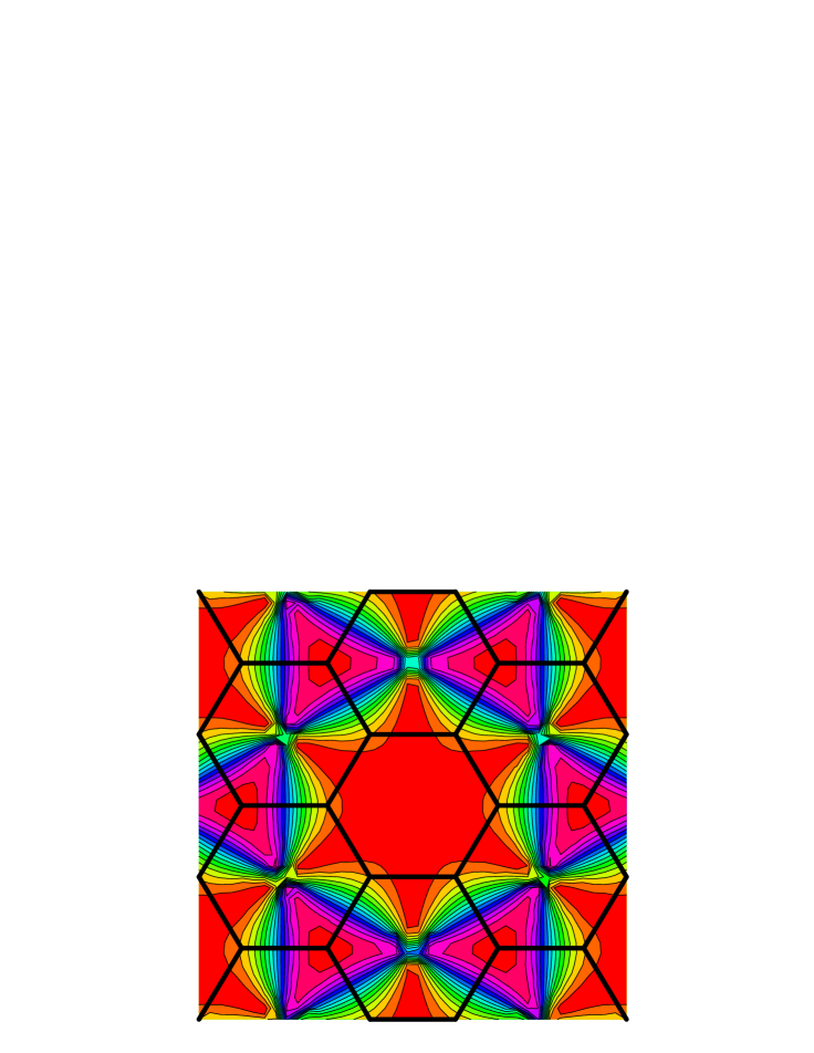
FIG. 9.: Neutron-scattering cross section from the large-$D$ kagomé antiferromagnet at $T=0$ (cf. Fig. 2).

\begin{picture}(11.0,7.0)\centerline{\hbox{\psfig{angle=-90,width=341.43306pt}}} \end{picture}

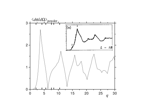
FIG. 10.: Powder average of the neutron-scattering cross section from the kagomé antiferromagnet at $T=0$. Inset: MC simulations of Ref. [15] for the Heisenberg model.

Let us now analyze the neutron cross section in more detail. At $T=0$ using Eqs. (16) and (55) one obtains

$$\frac{d\sigma}{d\Omega}=\frac{4\sin^{2}(q_{x}/2)[\cos(q_{x}/2)-\cos(\sqrt{3}q_{y}/2)]^{2}}{\sin^{2}(q_{x})+\sum_{\pm}\sin^{2}(q_{x}/2\pm\sqrt{3}q_{y}/2)},$$ (101)

where $\sum_{\pm}$ sums terms with both signs. Particular cases of this formula are the following. For $q_{y}=0$ one has

$$\frac{d\sigma}{d\Omega}=\frac{4\sin^{4}(q_{x}/4)}{1+2\cos^{2}(q_{x}/2)}.$$ (102)

This is equal to 1/3 at the corner of the first BZ, $q_{x}=2\pi/3$, to 2 at $q_{x}=\pi$ (the highest slope), to 3 at $q_{x}=4\pi/3$ (the maximum), and to 8/3 at $q_{x}=2\pi$. Near the line $q_{x}=0$, Eq. (101) simplifies to

$$\frac{d\sigma}{d\Omega}\cong\frac{q_{x}^{2}}{2}\tan^{2}\frac{\sqrt{3}q_{y}}{4},\qquad q_{y},\left|q_{y}-\frac{2\pi}{\sqrt{3}}\right|\gg q_{x}.$$ (103)

For small wave vectors one obtains

$$\frac{d\sigma}{d\Omega}\cong\frac{1}{96}\frac{q_{x}^{2}(q_{x}^{2}-3q_{y}^{2})^{2}}{q_{x}^{2}+q_{y}^{2}},\qquad q_{x},q_{y}\ll 1.$$ (104)

The most interesting form of the neutron cross section is realized in the vicinity of the centers of the Brillouin zones surrounding the first BZ in Fig. 9. In particular, near ${\bf q}=(0,2\pi/\sqrt{3})$ Eq. (101) takes the form

$$\frac{d\sigma}{d\Omega}\cong\frac{8}{3}\frac{q_{x}^{2}}{q_{x}^{2}+(\delta q_{y})^{2}},\qquad q_{x},\delta q_{y}\ll 1,$$ (105)

where $\delta q_{y}\equiv q_{y}-2\pi/\sqrt{3}$. This function is nonanalytic at $q_{x},\delta q_{y}=0$, and its limiting value in this point depends on the way of approaching to. (Such a function is difficult to plot: What looks like narrow paths in Fig. 9 are in fact infinitely thin walls.)

At $T\neq 0$ one should take into account the terms with $n=2,3$ in Eq. (100). This is especially important in the region where the zero-temperature neutron cross section turns to zero or is singular. In particular, near ${\bf q}=0$ the quantity $W_{1}^{2}$ is small due to cancellation of the leading terms and is given by the right-hand side (rhs) of Eq. (104). Similar cancellation takes place in $W_{2}^{2}$, and the result is given by the same formula with interchanged $q_{x}$ and $q_{y}$. The leading term thus becomes the noncancelled one associated with the “optical” eigenvalue, $W_{3}^{2}=3$. This leads to the uniform susceptibility given by Eqs. (56) and (63), that tends to a constant in the low-temperature limit. On the contrary, $\chi_{\bf q}$ with ${\bf q}\neq 0$ behaves as $1/T$ at low temperatures.

In the vicinity of the singularity point ${\bf q}=(0,2\pi/\sqrt{3})$, i.e., near the center of the Brillouin zone just above the first (central) BZ in Fig. 9, cancellation of the leading terms does not take place. Here the matrix $\hat{U}_{\bf q}$ differs from that of Eq. (20) by the redefinition $n_{y}\equiv\delta q_{y}/[q_{x}^{2}+(\delta q_{y})^{2}]^{1/2}$ and by the change of sign of the third row. Here $W_{2}^{2}$ is given by the rhs of Eq. (105) with interchanged $q_{x}$ and $\delta q_{y}$. Now with the use of Eq. (67) one obtains the final result

$$\frac{d\sigma}{d\Omega}\cong\frac{8}{3}\frac{\kappa^{2}+q_{x}^{2}}{\kappa^{2}+q_{x}^{2}+(\delta q_{y})^{2}},\qquad\kappa,q_{x},\delta q_{y}\ll 1.$$ (106)

It can be seen that this expression is nonanalytic only in the limit $T\to 0$, where the correlation length $\xi_{c}$ defined by Eq. (68) becomes infinite.

The powder average of the neutron cross section $\langle d\sigma/d\Omega\rangle$, i.e., the average of Eq. (100) over the directions of ${\bf q}$, is shown in Fig. 10. Positions of its singularities at $T=0$ can be found from the scattering pattern in Fig. 9. The first of them are located at $q=2\pi/\sqrt{3}\approx 3.63$ (sharp maximum), $2\pi\approx 6.28$ (sharp minimum), $\sqrt{(3\pi)^{2}+(\pi/\sqrt{3})^{2}}=2\pi\sqrt{7/3}\approx 9.6$ (small cuspy shoulder), $3\times 2\pi/\sqrt{3}\approx 10.88$ (sharp maximum), $\sqrt{(4\pi)^{2}+(2\pi/\sqrt{3})^{2}}=2\pi\sqrt{13/3}\approx 13.08$ (sharp minimum), $\sqrt{(5\pi)^{2}+(\pi/\sqrt{3})^{2}}=2\pi\sqrt{19/3}\approx 15.81$ (sharp maximum), $5\times 2\pi/\sqrt{3}\approx 18.14$ (sharp maximum), $6\pi\approx 18.85$ (cuspy shoulder), etc. With increasing of $q$ the behavior of $\langle d\sigma/d\Omega\rangle$ becomes more and more irregular, and it very slowly approaches the value 1. The latter can be understood since for large values of $q$ the average over the directions of ${\bf q}$ should be equal to that over ${\bf q}$ itself. The latter is according to Eq. (99) nothing else but the autocorrelation function, and the result is unity for the normalization of $d\sigma/d\Omega$ adopted in Eq. (100).

At nonzero temperatures, the sharp features of $\langle d\sigma/d\Omega\rangle$ smoothen. Their low-temperature forms can be found with the help of Eq. (106) and are given by

$$\left\langle\frac{d\sigma}{d\Omega}\right\rangle\cong 2.712+0.868\delta q-\frac{4\sqrt{3}}{\pi}\frac{(\delta q)^{2}}{\sqrt{\kappa^{2}+(\delta q)^{2}}}$$ (107)

near the first maximum, $\delta q\equiv q-2\pi/\sqrt{3}$, and

$$\left\langle\frac{d\sigma}{d\Omega}\right\rangle\cong 0.0183-0.238\delta q+\frac{4}{\pi}\sqrt{\kappa^{2}+(\delta q)^{2}}$$ (108)

near the first minimum, $\delta q\equiv q-2\pi$. In the high-temperature limit, Eq. (99) is dominated by the autocorrelation function, and the neutron cross section defined by Eq. (100) is equal to 1 for all ${\bf q}$ (an absolutely diffuse scattering).

The MC simulation data of Ref. [15] for the Heisenberg model at $T=0.002J$ are shown in the inset to Fig. 10. At such low temperatures the system shows a tendency towards selection of the $\sqrt{3}\times\sqrt{3}$ phase, and the corresponding Bragg-reflection peaks grow. The latter, according Eq. (7), are situated at the corners of all Brillouin zones in the extended BZ scheme shown in Fig. 9, and their positions are shown by additional tics in Fig. 10. These peaks that are superimposed on the underlying $D=\infty$ structure can be traced out in the inset. Note that there are Bragg-reflection peaks in the vicinity of the $D=\infty$ peaks, and they seem to be mixed together in the simulations of Ref. [15]. In contrast, the first two minima in Fig. 10 can be found in the inset at nearly the same positions, although in a strongly rounded form.

VII Discussion

In the main part of this article, we have presented in detail the exact solution for the $D=\infty$ component classical antiferromagnet on the kagomé lattice. The solution does not show ordering at any temperature due to the strong degeneracy of the ground state, and the thermodynamic functions behave smoothly. In contrast to conventional two-dimensional magnets, there is no extended short-range order at low temperatures, and $T=0$ is not a critical point of the system. Although the correlation length diverges as $\xi_{c}\propto T^{-1/2}$, the power-law decay $\langle{\bf s}_{0}{\bf s}_{\bf r}\rangle\propto 1/r^{2}$ of the spin correlation functions leads to the loss of correlations at the scale of the interatomic distance. The magnetic neutron-scattering cross section becomes nonanalytic at $T\to 0$ but does not diverge at any “ordering” wave vector.

Although the model with an infinite number of spin components may appear very unphysical at the first glance, it is in fact the second that should be applied, after the mean-field approximation, to any classical spin system. It properly describes the effect of would be Goldstone modes and thus it has important advantages against the MFA. Properly scaled physical quantities show a smooth dependence on $D$, and in typical cases the large-$D$ model proves to be a reasonable approximation to the realistic one with $D=3$. So, the results for the heat capacity and the uniform susceptibility obtained above are in a fairly good agreement with the MC simulation results for the Heisenberg model in the whole temperature range. This implies that the $1/D$ corrections to the thermodynamic functions of the kagomé AFM, which could be studied within the same theoretical framework, [30, 31] are suppressed by some mechanism.

The $D=\infty$ model and the $1/D$ expansion seem to be inefficient in the cases when, due to topological effects, the behavior of the system abruptly changes at small values of $D$. A well-known example is the Berezinskii-Kosterlitz-Thouless transition which takes place in two dimensions for $D=2$. For the kagomé lattice, thermal fluctuations favor the $\sqrt{3}\times\sqrt{3}$ phase at low temperatures for the Heisenberg model, but there is no such an effect for $D>3$. [14, 16] On the other hand, the tendency to the selection of the $\sqrt{3}\times\sqrt{3}$ phase at low temperatures is already seen in the high-temperature series expansion of Ref. [7] for any finite value of $D$. Exactly how this mechanism becomes inefficient at low temperatures for $D>3$, could be studied with the help of the $1/D$ expansion. The latter describes lifting of the degeneracy of the largest eigenvalue of the correlation matrix in the first order in $1/D$ and is applicable in the whole range of temperatures.

As follows from the consideration above, the Heisenberg antiferromagnet on the kagomé lattice is still not the best model to substitute it with the $D=\infty$ model. For the Heisenberg AFM on the pyrochlore lattice, the large-$D$ approximation can be expected to work even better since this model is, in a sense, more disordered, and topological effects leading here to the selection of the coplanar phase arise only for $D=2$. [16] The formalism for the pyrochlore lattice in zero field is essentially the same as for the kagomé lattice, and the corresponding results will be presented elsewhere.

REFERENCES

- [1]
-
[2]
Permanent address: I. Institut für Theoretische Physik, Universität
Hamburg, Jungius Strasse 9, D-20355 Hamburg, Germany.
Electronic addresses: garanin@mpipks-dresden.mpg.de
garanin@physnet.uni-hamburg.de
http://www.mpipks-dresden.mpg.de/garanin/ - [3] Electronic address: canals@mpipks-dresden.mpg.de
- [4] J. N. Reimers, A. J. Berlinsky, and A.-C. Shi, Phys. Rev. B 43, 865 (1991).
- [5] J. T. Chalker, P. C. W. Holdsworth, and E. F. Shender, Phys. Rev. Lett. 68, 855 (1992).
- [6] J. N. Reimers, Phys. Rev. B 45, 7287 (1992).
- [7] A. B. Harris, C. Kallin, and A. J. Berlinsky, Phys. Rev. B 45, 2899 (1992).
- [8] C. Zeng and V. Elser, Phys. Rev. B 42, 8436 (1990).
- [9] J. N. Reimers, Phys. Rev. B 46, 193 (1992).
- [10] A. P. Ramirez, Annu. Rev. Mater. Sci. 24, 453 (1994).
- [11] P. Schiffer and A. P. Ramirez, Comments Condens. Mater. Phys. 18, 21 (1996).
- [12] J. N. Reimers, J. E. Greedan, and M. Björgvinsson, Phys. Rev. B 45, 7295 (1992).
- [13] Ch. Pich, Ph. D. thesis, Technische Universität München, 1994.
- [14] D. A. Huse and A. D. Rutenberg, Phys. Rev. B 45, 7536 (1992).
- [15] J. N. Reimers and A. J. Berlinsky, Phys. Rev. B 48, 9539 (1993).
- [16] R. Moessner and J. T. Chalker, Phys. Rev. Lett. 80, 2929 (1998).
- [17] A. V. Chubukov, Phys. Rev. Lett. 69, 832 (1992).
- [18] S. Sachdev, Phys. Rev. B 45, 12377 (1992).
- [19] P. W. Leung and V. Elser, Phys. Rev. B 47, 5459 (1993).
- [20] P. Lecheminant, B. Bernu, C. Lhuillier, L. Pierre, and P. Sindzingre, Phys. Rev. B 56, 2521 (1997).
- [21] J. von Delft and Ch. L. Henley, Phys. Rev. Lett. 69, 3236 (1992); Phys. Rev. B 48, 965 (1993).
- [22] H. E. Stanley, Phys. Rev. Lett. 20, 589 (1968).
- [23] H. E. Stanley, in Phase Transitions and Critical Phenomena, edited by C. Domb and M. S. Green (Academic Press, New York, 1974), Vol. 3.
- [24] H. E. Stanley, Phys. Rev. 176, 718 (1968).
- [25] T. N. Berlin and M. Kac, Phys. Rev. 86, 821 (1952).
- [26] G. S. Joyce, in Phase Transitions and Critical Phenomena, edited by C. Domb and M. S. Green (Academic Press, New York, 1972), Vol. 2.
- [27] R. Abe, Prog. Theor. Phys. 48, 1414 (1972); 49, 113 (1973).
- [28] R. Abe and S. Hikami, Prog. Theor. Phys. 49, 442 (1973); 57, 1197 (1977).
- [29] Y. Okabe and M. Masutani, Phys. Lett. A 65, 97 (1978).
- [30] D. A. Garanin, J. Stat. Phys. 74, 275 (1994).
- [31] D. A. Garanin, J. Stat. Phys. 83, 907 (1996).
- [32] D. A. Garanin and V. S. Lutovinov, Solid State Commun. 50, 219 (1984).
- [33] D. A. Garanin, Phys. Rev. B 53, 11593 (1996).
- [34] D. A. Garanin, J. Phys. A: Math. Gen. 29, L257 (1996).
- [35] D. A. Garanin, J. Phys. A: Math. Gen. 29, 2349 (1996).
- [36] M. N. Barber and M. E. Fisher, Ann. Phys. (N.Y.) 77, 1 (1973).
- [37] D. A. Garanin, Z. Phys. B 102, 283 (1997).
- [38] A. Auerbach and D. P. Arovas, Phys. Rev. Lett. 61, 617 (1988); Phys. Rev. B 38, 316 (1988).
- [39] C. Timm, S. M. Girvin, and P. Henelius, Phys. Rev. B 58, 1464 (1998).
- [40] S. Chakravarty, B. I. Halperin, and D. R. Nelson, Phys. Rev. Lett. 60, 1057 (1988); Phys. Rev. B 39, 2344 (1989).
- [41] A. V. Chubukov, S. Sachdev, and J. Ye, Phys. Rev. B 49, 11919 (1994).
- [42] A. V. Chubukov and O. A. Starykh, cond-mat/9802291.
- [43] S. Ma, Modern Theory of Critical Phenomena (Benjamin, New York, 1973).
- [44] A. J. Bray and M. A. Moore, Phys. Rev. Lett. 38, 735 (1977); J. Phys. A: Math. Gen. 10, 1927 (1977).
- [45] D. A. Garanin, Phys. Rev. E 58, 254 (1998).
- [46] A. Pimpinelli and E. Rastelli, Phys. Rev. B 42, 984 (1990).
- [47] M. P. Zinkin, M. J. Harris, and T. Zeiske, Phys. Rev. B 56, 11786 (1997).
- [48] B. Canals and C. Lacroix, Phys. Rev. Lett. 80, 2933 (1998).