Abstract

A stochastic model for behavioral changes by imitative pair interactions of individuals is developed. ‘Microscopic’ assumptions on the specific form of the imitative processes lead to a stochastic version of the game dynamical equations. That means, the approximate mean value equations of these equations are the game dynamical equations of evolutionary game theory.

The stochastic version of the game dynamical equations allows the derivation of covariance equations. These should always be solved along with the ordinary game dynamical equations. On the one hand, the average behavior is affected by the covariances so that the game dynamical equations must be corrected for increasing covariances. Otherwise they may become invalid in the course of time. On the other hand, the covariances are a measure for the reliability of game dynamical descriptions. An increase of the covariances beyond a critical value indicates a phase transition, i.e. a sudden change in the properties of the considered social system.

The applicability and use of the introduced equations are illustrated by computational results for the social self-organization of behavioral conventions.

Keywords: evolutionary game theory, behavioral model, imitative processes, self-organization of behavioral conventions, stochastic game theory, mean value equations, covariance equations, reliability of rate equations, expected strategy distribution, most probable strategy distribution

1 Introduction

This paper treats a mathematical model for the temporal change of the proportions of individuals showing certain behavioral strategies. Models of this kind are of special interest for a quantitative understanding or prognosis of social developments. For the description of the competition or cooperation in populations there already exist game theoretical approaches (cf. e.g. von Neumann and Morgenstern, 1944; Luce and Raiffa, 1957; Rapoport and Chammah, 1965; Axelrod, 1984). In order to cope with time-dependent problems the method of iterated games has been developed and used for a long time. However, some years ago, the game dynamical equations have been discovered (Taylor and Jonker, 1978; Hofbauer et. al., 1979; Zeeman, 1980). These are ordinary differential equations, which are related to the theory of evolution (Eigen, 1971; Fisher, 1930; Eigen and Schuster, 1979; Hofbauer and Sigmund, 1988; Feistel and Ebeling, 1989). Therefore, one also speaks of evolutionary game theory.

The game dynamical equations have the following advantages:

• They are continuous in time which is more adequate for many problems.

• Ordinary differential equations are easier to handle than iterated formulations.

• Analytical results can be derived more easily (cf. e.g. Hofbauer and Sigmund, 1988; Helbing, 1992).

Up to now, there only exists a ‘macroscopic’ foundation of the game dynamical equations, i.e. a derivation from a collective level of behavior (cf. Section 5.1). In this paper a ‘microscopic’ foundation will be given, i.e. a derivation on the basis of the individual behavior. With this aim in view, we will first develop a stochastic behavioral model for the following reasons:

• A stochastic model, i.e. a model that can describe random fluctuations of the quantities of interest, can cope with the fact that behavioral changes are not exactly predictable (which is a consequence of the ‘freedom of decision-making’).

• The phenomena appearing in the considered social system can be connected to the principles of individual behavior. As a consequence, processes on the ‘macroscopic’ (collective) level can be understood as effects of ‘microscopic’ (individual) interactions.

• The probability of occurence of each strategy can be calculated. This is especially important for small social systems which are subject to large fluctuations (since they consist of a few individuals only).

• The stochastic model allows the derivation of covariance equations (cf. Section 4). Since the covariances influence the average temporal behavior, they are an essential criterium for the validity and reliability of behavioral descriptions by rate equations (which are actually approximate mean value equations). If the covariances exceed a certain critical value, this indicates the occurence of a phase transition, i.e. a sudden change of the properties of the considered social system.

For the description of systems that are subject to random fluctuations different stochastic methods have been developed (cf. e.g. Gardiner, 1983; Weidlich and Haag, 1983; Helbing, 1992). One method is to delineate the temporal evolution of the probability distribution over the different possible states (which represent behavioral strategies, here). This method is particularly suitable for an ‘ensemble’ of similar systems or for frequently occuring processes. In the case of discrete states, the master equation has to be used, whereas in the case of continuous state variables the Fokker-Planck equation is normally preferred since it is easier to handle (Fokker, 1914; Planck, 1917). The Fokker-Planck equation can, in good approximation, also be applied to systems with a large number of discrete states if state changes only occur between neighbouring states. It can be derived from the master equation by a Kramers-Moyal expansion (Kramers, 1940; Moyal, 1949), i.e. a second order Taylor approximation, then.

Another method, the Langevin equation (1908) (or stochastic differential equation) is applied to the description of the temporal evolution of single fluctuation-affected systems. It consists of a deterministic dynamical part which delineates systematic state changes and a stochastic fluctuation term which reflects random state variations. The Langevin equation can be reformulated in terms of a Fokker-Planck equation and vice versa (if the fluctuations are Gaussian and $\delta$-correlated which is normally the case; cf. Stratonovich, 1963, 1967; Weidlich and Haag, 1983).

Although these methods come from statistical physics, the application to interdisciplinary topics has meanwhile a long and successful tradition, beginning with the work of Weidlich (1971, 1972), Haken (1975), Prigogine (1976), Nicolis and Prigogine (1977). Also for social and economic processes Fokker-Planck equation models (cf. e.g. Weidlich and Haag, 1983; Topol, 1991) as well as master equation models (cf. e.g. Weidlich and Haag, 1983; Weidlich, 1991; Haag et.al., 1993; Weidlich and Braun, 1992) were proposed. In this paper we will develop a behavioral model on the basis of the master equation (Section 2). For this purpose we have to specify the transition rates, i.e. the probabilities per time unit with which changes of behavioral strategies take place. The transition rates can be decomposed into

• rates describing spontaneous strategy changes, and

• rates describing strategy changes due to pair interactions of individuals.

In the following we will restrict our considerations to imitative pair interactions which seem to be the most important ones (Helbing, 1994). By distinguishing several subpopulations $a$, different types of behavior or different groups of individuals can be taken into account.

In order to connect the stochastic behavioral model to the game dynamical equations the transition rates have to be chosen in such a way that they depend on the expected successes of the behavioral strategies (cf. Section 3.2). The ordinary game dynamical equations are the approximate mean value equations of the stochastic behavioral model (cf. Section 5.2).

For the approximate mean value equations correction terms can be calculated. These depend on the covariances (of the numbers of individuals pursuing a certain strategy) (cf. Section 4.1.4). Neglecting these corrections, the game dynamical equations may lose their validity after some time. The calculation of the covariances allows the determination of the time interval during which game dynamical descriptions are reliable (cf. Section 4.1.5).

The introduced equations are illustrated by computational results for the self-organization of a behavioral convention by a competition between two alternative, but equivalent strategies (cf. Sections 3.3 and 4). These results are relevant for economics with respect to the rivalry between similar products (Arthur, 1988, 1989; Hauk, 1994).

2 The stochastic behavioral model

Suppose we consider a social system with $N$ individuals. These individuals can be divided into $A$ subpopulations $a$ consisting of $N_{a}$ individuals, i.e.

$$\sum_{a=1}^{A}N_{a}=N\,.$$

By subpopulations different social groups (e.g. blue and white collars) or different characteristic types of behavior are distinguished. In the following we will assume that individuals of the same subpopulation (group) behave cooperatively due to common interests, whereas individuals of different subpopulations (groups) do not so due to conflicting interests.

The $N_{a}$ individuals of each subpopulation $a$ are distributed over several states

$$i\in\{1,\dots,S\}$$

which represent the alternative (behavioral) strategies of an individual. For the time being, every individual shall be able to choose each of the $S$ strategies, i.e. the same strategy set shall be available for each subpopulation. If the occupation number $n_{i}^{a}(t)$ denotes the number of individuals of subpopulation $a$ who use strategy $i$ at the time $t$, we have the relation

$$\sum_{i=1}^{S}n_{i}^{a}(t)=N_{a}\,.$$ (1)

Let

$$\mbox{\boldmath$n$}:=(n_{1}^{1},\dots,n_{i}^{a},\dots,n_{S}^{A})$$

be the vector consisting of all occupation numbers $n_{i}^{a}$. This vector is called the socioconfiguration since it contains all information about the distribution of the $N$ individuals over the states $i$. $P(\mbox{\boldmath$n$},t)$ shall denote the probability to find the socioconfiguration $n$ at the time $t$. This implies

$$0\leq P(\mbox{\boldmath$n$},t)\leq 1\qquad\mbox{and}\qquad\sum_{n}P(\mbox{\boldmath$n$},t)=1\,.$$

If transitions from socioconfiguration $n$ to $\mbox{\boldmath$n$}^{\prime}$ occur with a probability of $P(\mbox{\boldmath$n$}^{\prime},t+\Delta t|\mbox{\boldmath$n$},t)$ during a short time interval $\Delta t$, we have a (relative) transition rate of

$$w(\mbox{\boldmath$n$}^{\prime}|\mbox{\boldmath$n$};t):=\lim_{\Delta t\rightarrow 0}\frac{P(\mbox{\boldmath$n$}^{\prime},t+\Delta t|\mbox{\boldmath$n$},t)}{\Delta t}\,.$$

The absolute transition rate of changes from $n$ to $\mbox{\boldmath$n$}^{\prime}$ is the product $w(\mbox{\boldmath$n$}^{\prime}|\mbox{\boldmath$n$};t)P(\mbox{\boldmath$n$},t)$ of the probability $P(\mbox{\boldmath$n$},t)$ to have configuration $n$ and the relative transition rate $w(\mbox{\boldmath$n$}^{\prime}|\mbox{\boldmath$n$};t)$ if having configuration $n$. Whereas the inflow into $n$ is given as the sum over all absolute transition rates of changes from an arbitrary configuration $\mbox{\boldmath$n$}^{\prime}$ to $n$, the outflow from $n$ is given as the sum over all absolute transition rates of changes from $n$ to another configuration $\mbox{\boldmath$n$}^{\prime}$. Since the temporal change of the probability $P(\mbox{\boldmath$n$},t)$ is determined by the inflow into $n$ reduced by the outflow from $n$, we find the socalled master equation

$$\frac{d}{dt}P(\mbox{\boldmath$n$},t) = \mbox{inflow into $\mbox{\boldmath$n$}$ }-\mbox{ outflow from $\mbox{\boldmath$n$}$}$$ (2)

$$= \sum_{n^{\prime}}w(\mbox{\boldmath$n$}|\mbox{\boldmath$n$}^{\prime};t)P(\mbox{\boldmath$n$}^{\prime},t)-\sum_{n^{\prime}}w(\mbox{\boldmath$n$}^{\prime}|\mbox{\boldmath$n$};t)P(\mbox{\boldmath$n$},t)\qquad$$

(Pauli, 1928; Haken, 1979; Weidlich and Haag, 1983; Weidlich, 1991).

It will be assumed that two processes contribute to a change of the socioconfiguration $n$:

• Individuals may change their strategy $i$ spontaneously and independently of each other to another strategy $i^{\prime}$ with an individual transition rate $\widehat{w}_{a}(i^{\prime}|i;t)$. These changes correspond to transitions of the socioconfiguration from $n$ to

  $$\mbox{\boldmath$n$}_{i^{\prime}i}^{a}:=(n_{1}^{1},\dots,(n_{i^{\prime}}^{a}+1),\dots,(n_{i}^{a}-1),\dots,n_{S}^{A})$$

  with a configurational transition rate $w(\mbox{\boldmath$n$}_{i^{\prime}i}^{a}|\mbox{\boldmath$n$};t)=n_{i}^{a}\widehat{w}_{a}(i^{\prime}|i;t)$ which is proportional to the number $n_{i}^{a}$ of individuals who can change strategy $i$.

• An individual of subpopulation $a$ may change the strategy from $i$ to $i^{\prime}$ during a pair interaction with an individual of some subpopulation $b$ who changes the strategy from $j$ to $j^{\prime}$. Let transitions of this kind occur with a probability $\widehat{w}_{ab}(i^{\prime},j^{\prime}|i,j;t)$ per time unit. The corresponding change of the socioconfiguration from $n$ to

  $$\mbox{\boldmath$n$}_{i^{\prime}j^{\prime}ij}^{ab}:=(n_{1}^{1},\dots,(n_{i^{\prime}}^{a}+1),\dots,(n_{i}^{a}-1),\dots,(n_{j^{\prime}}^{b}+1),\dots,(n_{j}^{b}-1),\dots,n_{S}^{A})$$

  leads to a configurational transition rate $w(\mbox{\boldmath$n$}_{i^{\prime}j^{\prime}ij}^{ab}|\mbox{\boldmath$n$};t)=n_{i}^{a}n_{j}^{b}\widehat{w}_{ab}(i^{\prime},j^{\prime}|i,j;t)$ which is proportional to the number $n_{i}^{a}n_{j}^{b}$ of possible pair interactions between individuals of subpopulations $a$ and $b$ who pursue strategy $i$ and $j$ respectively. (Exactly speaking—in order to exclude self-interactions—$n_{i}^{a}n_{i}^{a}\widehat{w}_{aa}(i^{\prime},j^{\prime}|i,i;t)$ has to be replaced by $n_{i}^{a}(n_{i}^{a}-1)\widehat{w}_{aa}(i^{\prime},j^{\prime}|i,i;t)$ if $\sum_{j^{\prime}}\widehat{w}_{aa}(i^{\prime},j^{\prime}|i,i;t)\ll\widehat{w}_{a}(i^{\prime}|i;t)$ is invalid and $P(\mbox{\boldmath$n$},t)$ is not negligible where $n_{i}^{a}\gg 1$ is not fulfilled.)

The resulting configurational transition rate $w(\mbox{\boldmath$n$}^{\prime}|\mbox{\boldmath$n$};t)$ is given by

$$w(\mbox{\boldmath$n$}^{\prime}|\mbox{\boldmath$n$};t):=\left\{\begin{array}[]{ll}n_{i}^{a}\widehat{w}_{a}(i^{\prime}|i;t)&\mbox{if }\mbox{\boldmath$n$}^{\prime}=\mbox{\boldmath$n$}_{i^{\prime}i}^{a}\\ n_{i}^{a}n_{j}^{b}\widehat{w}_{ab}(i^{\prime},j^{\prime}|i,j;t)&\mbox{if }\mbox{\boldmath$n$}^{\prime}=\mbox{\boldmath$n$}_{i^{\prime}j^{\prime}ij}^{ab}\\ 0&\mbox{otherwise.}\end{array}\right.$$ (3)

As a consequence, the explicit form of master equation (2) is

$$\frac{d}{dt}P(\mbox{\boldmath$n$},t) = \sum_{a,i,i^{\prime}}\Big{[}(n_{i^{\prime}}^{a}+1)\widehat{w}_{a}(i|i^{\prime};t)P(\mbox{\boldmath$n$}_{i^{\prime}i}^{a},t)-n_{i}^{a}\widehat{w}_{a}(i^{\prime}|i;t)P(\mbox{\boldmath$n$},t)\Big{]}$$ (4)

$$+ \frac{1}{2}\sum_{a,i,i^{\prime}}\sum_{b,j,j^{\prime}}\Big{[}(n_{i^{\prime}}^{a}+1)(n_{j^{\prime}}^{b}+1)\widehat{w}_{ab}(i,j|i^{\prime},j^{\prime};t)P(\mbox{\boldmath$n$}_{i^{\prime}j^{\prime}ij}^{ab},t)$$

$$\qquad\qquad-\;n_{i}^{a}n_{j}^{b}\widehat{w}_{ab}(i^{\prime},j^{\prime}|i,j;t)P(\mbox{\boldmath$n$},t)\Big{]}$$

(cf. Helbing, 1992a).

We restricted our considerations to pair interactions, here, since they normally play the most significant role. Even in groups the most frequent interactions are alternating pair interactions—not always but in many cases. In situations where simultaneous interactions between more than two individuals are essential (one example for this is group pressure), the above master equation must be extended by higher order interaction terms. The corresponding procedure is discussed by Helbing (1992, 1992a).

3 Stochastic version of the game dynamical equations

3.1 Specification of the transition rates

The pair interactions

$$i^{\prime},j^{\prime}\longleftarrow i,j$$ (5)

of two individuals of subpopulations $a$ and $b$ who change their strategy from $i$ and $j$ to $i^{\prime}$ and $j^{\prime}$ respectively can be classified into three different kinds of processes: Imitative processes, avoidance processes, and compromising processes. These are discussed in detail and simulated in several publications (Helbing, 1992, 1992b, 1994). In the following we will focus to imitative processes (processes of persuasion) which describe the tendency to take over the strategy of another individual. These are of the special form

$$i,i\longleftarrow i,j (i\neq j)\,,$$ (6a)

$$j,j\longleftarrow i,j (i\neq j)\,.$$ (6b)

The corresponding pair interaction rates read

$$\widehat{w}_{ab}(i^{\prime},j^{\prime}|i,j;t) = \widehat{\nu}_{ab}p_{ba}(i|j;t)\delta_{ii^{\prime}}\delta_{ij^{\prime}}(1-\delta_{ij})$$ (7a)

$$+ \widehat{\nu}_{ab}p_{ab}(j|i;t)\delta_{jj^{\prime}}\delta_{ji^{\prime}}(1-\delta_{ij})\,,$$ (7b)

where the Kronecker symbol $\delta_{ij}$ is defined by

$$\delta_{ij}:=\left\{\begin{array}[]{ll}1&\mbox{if }i=j\\ 0&\mbox{if }i\neq j\,.\end{array}\right.$$

The factors $(1-\delta_{ij})$ result from the constraint $i\neq j$, whereas factors of the form $\delta_{ij}$ correspond to conditions of the kind $i=j$ which follow by comparison of (5a) and (5b) respectively with (5). The parameter

$$\nu_{ab}:=N_{b}\,\widehat{\nu}_{ab}$$ (8)

represents the contact rate between an individual of subpopulation $a$ with individuals of subpopulation $b$. $p_{ab}(j|i;t)$ denotes the probability of an individual of subpopulation $a$ to change the strategy from $i$ to $j$ during an imitative pair interaction with an individual of subpopulation $b$, i.e.

$$\sum_{j}p_{ab}(j|i;t)=1\,.$$

For $j\neq i$ we will assume

$$p_{ab}(j|i;t):=f_{ab}\widehat{R}_{a}(j|i;t)$$ (9)

where the parameter $f_{ab}$ is a measure for the frequency of imitative pair interactions between individuals of subpopulation $a$ when confronted with an individual of subpopulation $b$. $\widehat{R}_{a}(j|i;t)$ is a measure for the readiness of individuals belonging to subpopulation $a$ to change the strategy from $i$ to $j$ during a pair interaction.

3.2 ‘Microscopic’ foundation of evolutionary game theory

The problem of this section is to specify the frequency $f_{ab}$ and the readiness $\widehat{R}_{a}(j|i;t)\equiv\widehat{R}_{a}(j|i;\mbox{\boldmath$n$};t)$ in an adequate way. For this we make the following assumptions:

• By experience each individual knows—at least approximately—the expected success of the strategy used: We will define the expected success of a strategy $i$ for an individual of subpopulation $a$ in interactions with other individuals by

  $$\widehat{E}_{a}(i,t)\equiv\widehat{E}_{a}(i,\mbox{\boldmath$n$};t):=\sum_{b}\sum_{j}r_{ab}E_{ab}(i,j)\frac{n_{j}^{b}(t)}{N_{b}}\,.$$ (10)

  Here, the parameter

  $$r_{ab}=\frac{\nu_{ab}}{\displaystyle\sum_{c}\nu_{ac}}$$

  represents the relative contact rate of an individual of subpopulation $a$ with individuals of subpopulation $b$. $n_{j}^{b}(t)/N_{b}$ is the probability that an interaction partner of subpopulation $b$ uses strategy $j$. $E_{ab}(i,j)$ is an exogenously given quantity that denotes the success of strategy $i$ for an individual of subpopulation $a$ during an interaction with an individual of subpopulation $b$ who uses strategy $j$. Since all these quantities can be determined by each individual, the evaluation of the expected success $\widehat{E}_{a}(i,t)$ is obviously possible.

• In interactions with individuals of the same subpopulation an individual tends to take over the strategy of another individual if the expected success would increase: When an individual who uses strategy $i$ meets another individual of the same subpopulation who uses strategy $j$, they compare their expected successes $\widehat{E}_{a}(i,t)$ and $\widehat{E}_{a}(j,t)$ respectively by exchange of their experiences. (Remember that individuals of the same subpopulation were assumed to cooperate.) The individual with strategy $i$ will imitate the other’s strategy $j$ with a probability $p_{ab}(j|i;t)$ that is growing with the expected increase

  $$\Delta_{ji}\widehat{E}_{a}:=\widehat{E}_{a}(j,t)-\widehat{E}_{a}(i,t)$$

  of success. If a change of strategy would imply a decrease of success ($\Delta_{ji}\widehat{E}_{a}<0$), the individual will not change the strategy $i$. Therefore, the readiness for replacing the strategy $i$ by $j$ during an interaction within the same subpopulation can be assumed to be

  $$\widehat{R}_{a}(j|i;t):=\max\Big{(}\widehat{E}_{a}(j,t)-\widehat{E}_{a}(i,t),0\Big{)}$$ (11)

  where $\max(x,y)$ is the maximum of the two numbers $x$ and $y$. This describes an individual optimization or learning process.

• In interactions with individuals of other subpopulations (who behave in a non-cooperative way) normally no imitative processes will take place: During these interactions the expected success $\widehat{E}_{b}(j,t)$ of the interaction partner can at best be estimated by observation since he will not tell his experiences. Moreover, due to different criteria for the grade of success, the expected success of a strategy $j$ will normally be varying with the subpopulation (i.e. $\widehat{E}_{a}(i,t)\neq\widehat{E}_{b}(i,t)$ for $a\neq b$). As a consequence, an imitation of the strategy of individuals belonging to another subpopulation would be very risky since it would probably be connected with a decrease of expected success. Hence the assumption

  $$f_{ab}:=\delta_{ab}=\left\{\begin{array}[]{ll}1&\mbox{if }a=b\\ 0&\mbox{if }a\neq b\,.\end{array}\right.$$ (12)

  will normally be justified.

  Relation (12) also results in cases where the strategies of the respective other subpopulations cannot be imitated due to different (disjunct) strategy sets. Then, we need not to assume that individuals of the same subpopulations cooperate, whereas individuals of different subpopulations do not.

In Section 5 it will turn out that the game dynamical equations are the approximate mean value equations of the stochastic behavioral model defined by (3.1) to (12). In this sense, the model of this section can be regarded as stochastic version of the game dynamical equations. Moreover, the assumptions made above are a ‘microscopic’ foundation of evolutionary game theory since they allow a derivation of the game dynamical equations on the basis of individual behavior patterns.

3.3 Self-organization of behavioral conventions by competition between strategies

As an example for the stochastic game dynamical equations we will consider a case with one subpopulation only ($A=1$). In this case we can omit the indices $a$, $b$, and the summation over $b$. Let us assume the individuals to choose between two equivalent strategies $i\in\{1,2\}$, i.e. the success matrix $\underline{E}\equiv\Big{(}E(i,j)\Big{)}$ is symmetrical:

$$\underline{E}:=\left(\begin{array}[]{cc}B+C&B\\ B&B+C\end{array}\right)\,.$$ (13)

According to the relation

$$n_{1}(t)+n_{2}(t)=N$$

(cf. (1)), $n_{2}(t)=N-n_{1}(t)$ is already determined by $n_{1}(t)$. For spontaneous strategy changes due to trial and error we will take the simplest form of transition rates:

$$w(j|i;t):=W\,.$$ (14)

A situation of the above kind is the avoidance behavior of pedestrians (cf. Helbing, 1991, 1992): In pedestrian crowds with two opposite directions of motion, pedestrians have sometimes to avoid each other in order to exclude a collision. For an avoidance maneuver to be successful, both pedestrians concerned have to pass the respective other pedestrian either on the right hand side (strategy $i=1$) or on the left hand side (strategy $i=2$). Otherwise, both pedestrians have to stop (cf. Figure 1a). Here, both strategies are equivalent, but the success of a strategy increases with the number $n_{i}$ of individuals who use the same strategy. In success matrix (13) we have

$$C>0\,,$$

then.

Empirically one finds that the probability $P_{1}$ of choosing the right hand side is usually different from the probability $P_{2}=1-P_{1}$ of choosing the left hand side. Consequently, opposite directions of motion normally use separate lanes (cf. Figure 1b).

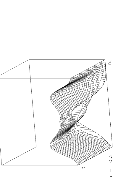
Figure 2: Probability distribution $P(\mbox{\boldmath$n$},t)\equiv P(n_{1},N-n_{1};t)$ of the socioconfiguration $n$ for varying values of the control parameter $\kappa$. For $\kappa=0$ a phase transition occurs: Whilst for $\kappa<0$ both strategies are used by about one half of the individuals, for $\kappa>0$ very probably one of the strategies will be prefered after some time. That means, a behavioral convention develops by social self-organization.

We will now examine if our behavioral model can explain this symmetry breaking (the fact that $P_{1}\neq P_{2}$). Figure 2 shows some computational results for $C=1$ and different values of $W/\nu$. If

$$\kappa:=1-\frac{4W}{\nu C}<0\,,$$ (15)

the configurational distribution is unimodal and symmetrical with respect to $n_{1}=N/2=n_{2}$, i.e. both strategies will be chosen by about one half of the individuals. At the critical point $\kappa=0$ there appears a phase transition (bifurcation). This is indicated by the broadness of the probability distribution $P(\mbox{\boldmath$n$},t)\equiv P(n_{1},n_{2};t)=P(n_{1},N-n_{1};t)$ which comes from socalled critical fluctuations (cf. Haken, 1983). The term ‘critical fluctuations’ denotes the fact that the fluctuations become particularly large at a critical point since the system behavior is unstable, then. Whereas the individuals behave more or less independently before the phase transition ($\kappa<0$), around the critical point the individuals begin to act correlated due to their (imitative) interactions. However, the spontaneous strategy changes (represented by $W$) still prevent the formation of a behavioral preference. Above the critical point (i.e. for $\kappa>0$) the correlation of individual behaviors is strong enough for the self-organization (emergence) of a behavioral convention: The configurational distribution becomes multimodal in the course of time with maxima at $n_{1}\neq N/2$ so that one of the two equivalent strategies will very probably be chosen by a majority of individuals. In this connection one also speaks of symmetry breaking (Haken, 1979, 1983).

Behavioral conventions often obtain a law-like character after some time. Which one of two equivalent strategies will win the majority is completely random. It is possible, that conventions differ from one region to another. This is, for example, the case for the prescribed driving direction of cars.

The model of this section can also be applied to the competition between the two video systems VHS and BETA MAX which were equivalent with respect to technology and price at the beginning (Hauk, 1994). In the course of time VHS won this rivalry since (for reasons of compatibility concerning copying, selling or hiring of video tapes) it was advantageous for new purchasers to decide for that video system which gained a small majority at some moment. Other examples for the emergence of a behavioral convention are the revolution direction of clock hands, the direction of writing, etc. A generalization of the above model to the case of more than two alternative strategies is easily possible. Of course, the model can also be adapted to situations where one behavioral alternative is superior to the others. However, the formation of a behavioral convention is trivial, then.

Finally, some related models should be mentioned which were proposed during the recent years for the description of symmetry breaking phenomena in economics: Orléan (1992, 1993) and Orléan and Robin (1992) presented a phase transition model using polynomial transition rates which base on a Bayesian rationale. Durlauf (1989, 1991) used Markovian fields to explain the non-ergodic (i.e. path-dependent) behavior of some economic systems. Föllmer (1974) applied the Ising model paradigm (1925) to model an economy of many interacting agents and discussed under which conditions a symmetry breakdown occurs. A similar model for polarization effects in opinion formation was already suggested by Weidlich (1972). Last but not least Topol (1991) presented a Fokker-Planck equation model for the explanation of bubbles in stock markets by mimetic contagion (i.e. some kind of imitative interactions) between agents.

4 Most probable and expected strategy distribution

Because of the huge number of possible socioconfigurations $n$, in more complex cases than in Section 3.3 the master equation for the determination of the configurational distribution $P(\mbox{\boldmath$n$},t)$ is usually difficult to solve (even with a computer). However,

• in cases of the description of single or rare social processes the most probable strategy distribution

  $$P_{i}^{a}(t):=\frac{\widehat{n}_{i}^{a}(t)}{N_{a}}$$ (16)

  is the quantity of interest whereas

• in cases of frequently occuring social processes the interesting quantity is the expected strategy distribution

  $$P_{i}^{a}(t):=\frac{\langle n_{i}^{a}\rangle_{t}}{N_{a}}\,.$$ (17)

$P_{i}^{a}(t)$ is the proportion of individuals within subpopulation $a$ using strategy $i$ so that

$$P_{i}^{a}(t)\geq 0\qquad\mbox{and}\qquad\sum_{i}P_{i}^{a}(t)=1\,.$$

Equations for the most probable occupation numbers $\widehat{n}_{i}^{a}(t)$ can be deduced from a Langevin equation (1908) for the temporal development of the socioconfiguration $\mbox{\boldmath$n$}(t)$. For the mean values $\langle n_{i}^{a}\rangle_{t}$ of the occupation numbers $n_{i}^{a}$ normally only approximate closed equations can be derived. A measure for the reliability of $\widehat{n}_{i}^{a}(t)$ and $\langle n_{i}^{a}\rangle_{t}$ with respect to the possible temporal developments of $n_{i}^{a}(t)$ are the variances $\sigma_{ii}^{aa}(t)$ of $n_{i}^{a}(t)$. If the standard deviation $\sqrt{\sigma_{ii}^{aa}(t)}$ becomes comparable to $0.12\widehat{n}_{i}^{a}(t)$ or $0.12\langle n_{i}^{a}\rangle_{t}$, the values of $\widehat{n}_{i}^{a}(t)$ and $\langle n_{i}^{a}\rangle_{t}$ respectively are not representable for $n_{i}^{a}(t)$ any more (cf. Section 4.1.5). In the case of $P(\mbox{\boldmath$n$},t)$ being normally distributed this would imply a probability of 34% (5%) that the value of $n_{i}^{a}(t)$ deviated more than 12% (24%) from $\widehat{n}_{i}^{a}(t)$ and $\langle n_{i}^{a}\rangle_{t}$ respectively. Moreover, if the variances $\sigma_{ii}^{aa}(t)$ become large, this may indicate a phase transition, i.e. a non-ergodic (path-dependent) temporal evolution of the system (see Figure 2).

4.1 Mean value and covariance equations

The mean value of a function $f(\mbox{\boldmath$n$},t)$ is defined by

$$\langle f(\mbox{\boldmath$n$},t)\rangle_{t}\equiv\langle f(\mbox{\boldmath$n$},t)\rangle:=\sum_{n}f(\mbox{\boldmath$n$},t)P(\mbox{\boldmath$n$},t)\,.$$

From master equation (4) can be derived that the mean values of the occupation numbers $f(\mbox{\boldmath$n$},t)=n_{i}^{a}$ are determined by the equations

$$\frac{d\langle n_{i}^{a}\rangle}{dt}=\langle m_{i}^{a}(\mbox{\boldmath$n$},t)\rangle$$ (18)

with the drift coefficients

$$m_{i}^{a}(\mbox{\boldmath$n$},t) := \sum_{n^{\prime}}(n^{\prime}{}_{i}^{a}-n_{i}^{a})w(\mbox{\boldmath$n$}^{\prime}|\mbox{\boldmath$n$};t)$$ (19)

$$= \sum_{i^{\prime}}\Big{[}\overline{w}^{a}(i|i^{\prime};t)n_{i^{\prime}}^{a}-\overline{w}^{a}(i^{\prime}|i;t)n_{i}^{a}\Big{]}$$

and the effective transition rates

$$\overline{w}^{a}(i^{\prime}|i;t):=\widehat{w}_{a}(i^{\prime}|i;t)+\sum_{b}\sum_{j^{\prime}}\sum_{j}\widehat{w}_{ab}(i^{\prime},j^{\prime}|i,j;t)n_{j}^{b}$$ (20)

(cf. Helbing, 1992, 1992a). Obviously, the contributions $\widehat{w}_{ab}(i^{\prime},j^{\prime}|i,j;t)n_{j}^{b}$ due to pair interactions are proportional to the number $n_{j}^{b}$ of possible interaction partners.

4.1.1 Approximate mean value equations

Equations (18) are no closed equations, since they depend on the mean values $\langle n_{i}^{a}n_{j}^{b}\rangle$, which are not determined by (18). We have, therefore, to find a suitable approximation. Using a first order Taylor approximation we obtain the approximate mean value equations

$$\frac{\partial\langle n_{i}^{a}\rangle}{\partial t} \approx \Bigg{\langle}m_{i}^{a}(\langle\mbox{\boldmath$n$}\rangle,t)+\sum_{b,j}(n_{j}^{b}-\langle n_{j}^{b}\rangle)\frac{\partial m_{i}^{a}(\langle\mbox{\boldmath$n$}\rangle,t)}{\partial\langle n_{j}^{b}\rangle}\Bigg{\rangle}$$ (21)

$$= m_{i}^{a}(\langle\mbox{\boldmath$n$}\rangle,t)\,.$$

These are applicable if the configurational distribution $P(\mbox{\boldmath$n$},t)$ has only small covariances

$$\sigma_{ij}^{ab} := \Big{\langle}(n_{i}^{a}-\langle n_{i}^{a}\rangle)(n_{j}^{b}-\langle n_{j}^{b}\rangle)\Big{\rangle}$$ (22)

$$= \langle n_{i}^{a}n_{j}^{b}\rangle-\langle n_{i}^{a}\rangle\langle n_{j}^{b}\rangle\approx 0\,.$$

Condition (22) corresponds to the limit of statistical independence $\langle n_{i}^{a}n_{j}^{b}\rangle=\langle n_{i}^{a}\rangle\langle n_{j}^{b}\rangle$ of the occupation numbers (and, therefore, of the individual behaviors).

4.1.2 Boltzmann-like equations

Inserting (17), (19), and (20) into (21) the resulting approximate equations for the expected strategy distribution $P_{i}^{a}(t)$ are

$$\frac{d}{dt}P_{i}^{a}(t)=\sum_{i^{\prime}}\Big{[}w^{a}(i|i^{\prime};t)P_{i^{\prime}}^{a}(t)-w^{a}(i^{\prime}|i;t)P_{i}^{a}(t)\Big{]}$$ (23)

with the mean transition rates

$$w^{a}(i^{\prime}|i;t)=\widehat{w}_{a}(i^{\prime}|i;t)+\sum_{b}\sum_{j^{\prime}}\sum_{j}N_{b}\,\widehat{w}_{ab}(i^{\prime},j^{\prime}|i,j;t)P_{j}^{b}(t)\,.$$ (24)

Equations (23), (24) are called Boltzmann-like equations (Boltzmann, 1964; Helbing, 1992, 1992a) since the mean transition rates (24) depend on the strategy distributions $P_{j}^{b}(t)$ due to pair interactions. Assuming (3.1), (8), and (9) we obtain the formula

$$w^{a}(i|i^{\prime};t)=\widehat{w}_{a}(i|i^{\prime};t)+R_{a}(i|i^{\prime};t)\sum_{b}\nu_{ab}f_{ab}P_{i}^{b}(t)$$ (25)

with $R_{a}(i|i^{\prime};t):=\widehat{R}_{a}(i|i^{\prime};\langle\mbox{\boldmath$n$}\rangle;t)$ for the mean transition rates. (23) and (25) are a special case of more general equations introduced by Helbing (1992, 1992b, 1994) for the temporal development of the expected strategy distribution in a social system consisting of a huge number $N\gg 1$ of individuals.

4.1.3 Approximate covariance equations

In many cases, the configuration $\mbox{\boldmath$n$}_{0}$ at an initial time $t_{0}$ is known by empirical evaluation, i.e. the initial distribution is

$$P(\mbox{\boldmath$n$},t_{0})=\delta_{nn_{0}}\,.$$

As a consequence, the covariances $\sigma_{ij}^{ab}$ vanish at time $t_{0}$ and remain small during a certain time interval. For the temporal development of $\sigma_{ij}^{ab}$, the equations

$$\frac{d\sigma_{ij}^{ab}}{dt}=\Big{\langle}m_{ij}^{ab}(\mbox{\boldmath$n$},t)\Big{\rangle}+\Big{\langle}(n_{i}^{a}-\langle n_{i}^{a}\rangle)m_{j}^{b}(\mbox{\boldmath$n$},t)\Big{\rangle}+\Big{\langle}(n_{j}^{b}-\langle n_{j}^{b}\rangle)m_{i}^{a}(\mbox{\boldmath$n$},t)\Big{\rangle}$$ (26)

can be derived from master equation (4) (cf. Helbing, 1992, 1992a). Here,

$$m_{ij}^{ab}(\mbox{\boldmath$n$},t) := \sum_{n^{\prime}}(n^{\prime}{}_{i}^{a}-n_{i}^{a})(n^{\prime}{}_{j}^{b}-n_{j}^{b})w(\mbox{\boldmath$n$}^{\prime}|\mbox{\boldmath$n$};t)$$ (27)

$$= \delta_{ab}\bigg{(}\delta_{ii^{\prime}}\sum_{j}\Big{[}n_{j}^{a}\overline{w}^{a}(i|j;t)+n_{i}^{a}\overline{w}^{a}(j|i;t)\Big{]}$$

$$\qquad-\;\Big{[}n_{i^{\prime}}^{a}\overline{w}^{a}(i|i^{\prime};t)+n_{i}^{a}\overline{w}^{a}(i^{\prime}|i;t)\Big{]}\bigg{)}$$

$$+ \sum_{j^{\prime}}\sum_{j}\Big{[}n_{j}^{a}n_{j^{\prime}}^{b}\widehat{w}_{ab}(i,i^{\prime}|j,j^{\prime};t)+n_{i}^{a}n_{i^{\prime}}^{b}\widehat{w}_{ab}(j,j^{\prime}|i,i^{\prime};t)\Big{]}\vphantom{\sum_{j}}$$

$$- \sum_{j^{\prime}}\sum_{j}\Big{[}n_{i}^{a}n_{j^{\prime}}^{b}\widehat{w}_{ab}(j,i^{\prime}|i,j^{\prime};t)+n_{j}^{a}n_{i^{\prime}}^{b}\widehat{w}_{ab}(i,j^{\prime}|j,i^{\prime};t)\Big{]}\qquad$$

are diffusion coefficients. Equations (26) are again no closed equations. However, a first order Taylor approximation of the drift and diffusion coefficients $m_{..}^{..}(\mbox{\boldmath$n$},t)$ leads to the equations

$$\frac{\partial\sigma_{ij}^{ab}}{\partial t}\approx m_{ij}^{ab}(\langle n\rangle,t)+\sum_{c,k}\Bigg{(}\sigma_{ik}^{ac}\frac{\partial m_{j}^{b}(\langle\mbox{\boldmath$n$}\rangle,t)}{\partial\langle n_{k}^{c}\rangle}+\sigma_{jk}^{bc}\frac{\partial m_{i}^{a}(\langle\mbox{\boldmath$n$}\rangle,t)}{\partial\langle n_{k}^{c}\rangle}\Bigg{)}\qquad$$ (28)

(cf. Helbing, 1992, 1992a) which are solvable together with (21). The approximate covariance equations (28) allow the determination of the time interval during which the approximate mean value equations (21) are valid (cf. Section 4.1.5 and Figures 5a, 5b). They are also useful for the calculation of the reliability (or representativity) of descriptions made by equations (21). Moreover, they are necessary for corrections of approximate mean value equations (21).

4.1.4 Corrected mean value and covariance equations

Equations (21) and (28) are only valid for the case

$$\Big{|}\sigma_{ij}^{ab}\Big{|}\ll\langle n_{i}^{a}\rangle\langle n_{j}^{b}\rangle$$ (29)

where the absolute values of the covariances $\sigma_{ij}^{ab}$ are small, i.e. where the configurational distribution $P(\mbox{\boldmath$n$},t)$ is sharply peaked. For increasing covariances a better approximation of (18) and (26) should be taken. A second order Taylor approximation of (18) and (26) respectively results in the corrected mean value equations

$$\frac{\partial\langle n_{i}^{a}\rangle}{\partial t}\approx m_{i}^{a}(\langle\mbox{\boldmath$n$}\rangle,t)+\frac{1}{2}\sum_{b,j}\sum_{c,k}\sigma_{jk}^{bc}\frac{\partial^{2}m_{i}^{a}(\langle\mbox{\boldmath$n$}\rangle,t)}{\partial\langle n_{j}^{b}\rangle\partial\langle n_{k}^{c}\rangle}\qquad$$ (30)

and the corrected covariance equations

$$\frac{d\sigma_{ij}^{ab}}{dt} \approx m_{ij}^{ab}(\langle n\rangle,t)+\frac{1}{2}\sum_{c,k}\sum_{d,l}\sigma_{kl}^{cd}\frac{\partial^{2}m_{ij}^{ab}(\langle\mbox{\boldmath$n$}\rangle,t)}{\partial\langle n_{k}^{c}\rangle\partial\langle n_{l}^{d}\rangle}\qquad$$ (31)

$$+ \sum_{c,k}\Bigg{(}\sigma_{ik}^{ac}\frac{\partial m_{j}^{b}(\langle\mbox{\boldmath$n$}\rangle,t)}{\partial\langle n_{k}^{c}\rangle}+\sigma_{jk}^{bc}\frac{\partial m_{i}^{a}(\langle\mbox{\boldmath$n$}\rangle,t)}{\partial\langle n_{k}^{c}\rangle}\Bigg{)}$$

(Helbing, 1992, 1992a). Note that the corrected mean value equations explicitly depend on the covariances $\sigma_{ij}^{ab}$, i.e. on the fluctuations due to the stochasticity of the processes described. They cannot be solved without solving the covariance equations. A comparison of (30) with (21) shows that the approximate mean value equations only agree with the corrected ones in the limit $\sigma_{ij}^{ab}$ of negligible corvariances (cf. also (22)). However, the calculation of the covariances is always recommendable since they are a measure for the reliability (or representativity) of the mean value equations. If the covariances become large in the sense of equation (33) this may indicate a phase transition.

4.1.5 Computational results

A comparison of exact, approximate and corrected mean value and variance equations is given in Figures 3 to 4a. These show computational results corresponding to the example of Section 3.3 (cf. Figure 2). Exact mean values $\langle n_{1}\rangle$ and variances $\sigma_{11}$ are represented by solid lines whereas approximate results according to (21), (28) are represented by dotted lines and corrected results according to (30), (31) by broken lines.

For $\kappa\geq 0$ the approximate mean value equations (21) become useless since the variances are growing due to the phase transition. As expected, the corrected mean value equations yield better results than the approximate mean value equations and they are valid for a longer time interval.

A criterium for the validity of the approximate equations (21), (28) and the corrected equations (30), (31) respectively are the relative central moments

$$C_{m}(t)\equiv C_{i_{1}}^{a_{1}}{}_{\dots}^{\dots}{}_{i_{m}}^{a_{m}}(t):=\frac{\Big{\langle}(n_{i_{1}}^{a_{1}}-\langle n_{i_{1}}^{a_{1}}\rangle)\cdot\dots\cdot(n_{i_{m}}^{a_{m}}-\langle n_{i_{m}}^{a_{m}}\rangle)\Big{\rangle}}{\langle n_{i_{1}}^{a_{1}}\rangle\cdot\dots\cdot\langle n_{i_{m}}^{a_{m}}\rangle}\,.$$

Whereas the approximate equations (21), (28) already fail, if

$$|C_{m}(t)|\leq 0.04$$ (32)

is violated for $m=2$ (compare to (29), (22)), the corrected equations (30), (31) presuppose condition (32) only for $3\leq m\leq l$ with a certain, well-defined value $l$ (cf. Helbing, 1992, 1992a for details). However, even the corrected equations (30), (31) become useless if the probability distribution $P(\mbox{\boldmath$n$},t)$ becomes multimodal, i.e. if a phase transition occurs. This is the case if

$$|C_{2}(t)|=\left|\frac{\sigma_{ij}^{ab}(t)}{\langle n_{i}^{a}\rangle\langle n_{j}^{b}\rangle}\right|\leq 0.12$$ (33)

is violated (cf. Figure 4).

4.2 Equations for the most probable strategy distribution

After the transformation of master equation (2) into a Fokker-Planck equation by a second order Taylor approximation, it can be reformulated in terms of a Langevin equation (1908) (cf. Weidlich and Haag, 1983; Helbing, 1992). The latter reads

$$\frac{d}{dt}n_{i}^{a}(t)\stackrel{{\scriptstyle N_{a}\gg 1}}{{=}}m_{i}^{a}(\mbox{\boldmath$n$},t)+\mbox{\em fluctuations}$$ (34)

and describes the temporal development of the socioconfiguration $\mbox{\boldmath$n$}(t)$ in dependence of process immanent fluctuations (that are determined by the diffusion coefficients $m_{ij}^{ab}$). As a consequence,

$$\frac{d}{dt}\widehat{n}_{i}^{a}(t)\stackrel{{\scriptstyle N_{a}\gg 1}}{{=}}m_{i}^{a}(\widehat{\mbox{\boldmath$n$}},t)$$ (35)

are the equations governing the temporal development of the most probable occupation numbers $\widehat{n}_{i}^{a}(t)$. Equations (35) look exactly like approximate mean value equations (21). Therefore, if $N_{a}\gg 1$, the approximate mean value equations have an interpretation even for large variances since they also describe the most probable strategy distribution.

5 The game dynamical equations

5.1 ‘Macroscopic’ derivation

Before we will connect the stochastic behavioral model to the game dynamical equations, we will discuss their derivation from a collective level of behavior. Let $E_{a}(i,t):=\widehat{E}_{a}(i,\langle\mbox{\boldmath$n$}\rangle;t)$ be the expected success of strategy $i$ for an individual of subpopulation $a$ and

$$\overline{E_{a}}(t):=\sum_{i}E_{a}(i,t)P_{i}^{a}(t)$$ (36)

the mean expected success. If the relative increase

$$\frac{dP_{i}^{a}/dt}{P_{i}^{a}(t)}$$

of the proportion $P_{i}^{a}(t)$ is assumed to be proportional to the difference $[E_{a}(i,t)-\overline{E_{a}}(t)]$ between the expected and the mean expected success, one obtains the game dynamical equations

$$\frac{d}{dt}P_{i}^{a}(t)=\nu_{a}P_{i}^{a}(t)\Big{[}E_{a}(i,t)-\overline{E_{a}}(t)\Big{]}\,.$$ (37)

According to these equations the proportions of strategies with an expected success that exceeds the average $\overline{E_{a}}(t)$ are growing, whereas the proportions of the remaining strategies are falling. For the expected success $E_{a}(i,t)$ one often takes the form

$$E_{a}(i,t):=\sum_{b}\sum_{j}A_{ab}(i,j)P_{j}^{b}(t)$$ (38)

where the quantities $A_{ab}(i,j)$ have the meaning of payoffs which are exogeneously determined. Consequently, the matrices

$$\underline{A}_{ab}:=\Big{(}A_{ab}(i,j)\Big{)}$$

are called payoff matrices. Inserting (36) and (38) into (37), one obtains the explicit form

$$\frac{d}{dt}P_{i}^{a}(t)=\nu_{a}P_{i}^{a}(t)\Bigg{[}\sum_{b,j}A_{ab}(i,j)P_{j}^{b}(t)-\sum_{i^{\prime}}\sum_{b,j}P_{i^{\prime}}^{a}(t)A_{ab}(i^{\prime},j)P_{j}^{b}(t)\Bigg{]}$$ (39)

of the game dynamical equations. Equations of this kind are very useful for the investigation and understanding of the competition or cooperation of individuals (cf. e.g. Hofbauer and Sigmund, 1988; Schuster et.al., 1981). Due to their nonlinearity they may have a complex dynamical solution, e.g. an oscillatory one (Hofbauer et.al., 1980; Hofbauer and Sigmund, 1988) or even a chaotic one (Schnabl et.al., 1991).

A slightly generalized form of (37),

$$\frac{d}{dt}P_{i}^{a}(t) = \sum_{i^{\prime}}\Big{[}\widehat{w}_{a}(i|i^{\prime};t)P_{i^{\prime}}^{a}(t)-\widehat{w}_{a}(i^{\prime}|i;t)P_{i}^{a}(t)\Big{]}$$ (40a)

$$+ \nu_{a}P_{i}^{a}(t)\Big{[}E_{a}(i,t)-\overline{E_{a}}(t)\Big{]}\,,\qquad$$ (40b)

is also known as selection mutation equation (Hofbauer and Sigmund, 1988): (40b) can be understood as effect of a selection (if $E_{a}(i,t)$ is interpreted as fitness of strategy $i$), and (40a) can be understood as effect of mutations. Equation (5.1) is a powerful tool in evolutionary biology (cf. Eigen, 1971; Fisher, 1930; Eigen and Schuster, 1979; Hofbauer and Sigmund, 1988; Feistel and Ebeling, 1989). In game theory, the mutation term could be used for the description of trial and error behavior or accidental variations of the strategy.

5.2 Derivation from the stochastic behavioral model

In this section we will look for a connection between the stochastic behavioral model of Section 3 and the game dynamical equations. For this purpose we compare the approximate mean value equations of this stochastic behavioral model, i.e. the Boltzmann-like equations (23), (25) with the game dynamical equations (5.1). Both equations will be identical only if

$$\nu_{ab}f_{ab}=\nu_{a}\delta_{ab}\,.$$

This condition corresponds to (12) if

$$\nu_{a}=\nu_{aa}\,.$$

Inserting assumptions (10) to (12) into the Boltzmann-like equations (23), (25) the game dynamical equations (5.1) result. We have only to introduce the identifications

$$A_{ab}(i,j):=r_{ab}E_{ab}(i,j)\,,$$

$$E_{a}(i,t):=\widehat{E}_{a}(i,\langle\mbox{\boldmath$n$}\rangle;t)=\sum_{b}\sum_{j}r_{ab}E_{ab}(i,j)P_{j}^{b}(t)\,,$$

and to apply the relation

$$\max\Big{(}E_{a}(i,t)-E_{a}(j,t),0\Big{)}-\max\Big{(}E_{a}(j,t)-E_{a}(i,t),0\Big{)}=E_{a}(i,t)-E_{a}(j,t)\,.$$

The game dynamical equations (including their properties and generalizations) are more explicitly discussed elsewhere (Helbing, 1992). An interesting application to a case with two subpopulations can be found in the book of Hofbauer and Sigmund (1988: pp. 137–146). In the following, we will again examine the example of Section 3.3 where we have one subpopulation and two equivalent strategies. The game dynamical equations (5.1) corresponding to (13) and (14) have, then, the explicit form

$$\frac{d}{dt}P_{i}(t)=-2\left(P_{i}(t)-\frac{1}{2}\right)\Big{[}W+\nu CP_{i}(t)\Big{(}P_{i}(t)-1\Big{)}\Big{]}\,.$$ (41)

According to (41), $P_{i}=1/2$ is a stationary solution. This solution is stable for

$$\kappa=1-\frac{4W}{\nu C}<0\,,$$

i.e. if spontaneous strategy changes are dominating and, therefore, prevent a self-organization process.

At the critical point $\kappa=0$ symmetry breaking appears: For $\kappa>0$ the stationary solution $P_{i}=1/2$ is unstable and the game dynamical equations (41) can be rewritten in the form

$$\frac{d}{dt}P_{i}(t)=-2\left(P_{i}(t)-\frac{1}{2}\right)\left(P_{i}(t)-\frac{1+\sqrt{\kappa}}{2}\right)\left(P_{i}(t)-\frac{1-\sqrt{\kappa}}{2}\right)\,.$$ (42)

This means, for $\kappa>0$ we have two additional stationary solutions $P_{i}=(1+\sqrt{\kappa})/2$ and $P_{i}=(1-\sqrt{\kappa})/2$ which are stable. Depending on initial fluctuations, one strategy will win a majority of $100\cdot\sqrt{\kappa}$ percent. This majority is the greater the smaller the rate $W$ of spontaneous strategy changes is.

6 Modified game dynamical equations

At first glance the crease of $P(n_{1},N-n_{1};t)$ at $n_{1}=N/2=n_{2}$ in the illustrations of Figure 2 appears somewhat surprising. A mathematical analysis shows that this is a consequence of the crease of the function $\widehat{R}_{a}(j|i;t)=\max(\widehat{E}_{a}(j,t)-\widehat{E}_{a}(i,t),0)$. It can be avoided by using the modified approach

$$\widehat{R}_{a}(j,i;t):=\frac{1}{2}\exp[\widehat{E}_{a}(j,t)-\widehat{E}_{a}(i,t)]\,.$$ (43)

(43) also leads to a phase transition for $\kappa=0$ (cf. Figure 6) and very similar results for the approximate mean value equations since the game dynamical equations result as Taylor approximation of those. According to (43), imitative strategy changes from $i$ to $j$ will again occur the more frequent the greater the expected increase $\Delta_{ji}\widehat{E}_{a}=\widehat{E}_{a}(j,t)-\widehat{E}_{a}(i,t)$ of success is.

Approach (43) originally stems from physics where the exponential function for the transition probability is due to the need to obtain the Boltzmann distribution (1964) as stationary distribution. Its application to behavioral changes was suggested by Weidlich (1971, 1972) in connection with a Ising-like (1925) opinion formation model. Meanwhile, related models were also proposed for economic systems (Haag et. al., 1993; Weidlich and Braun, 1992; Durlauf, 1989, 1991). In contrast to this, Orléan (1992, 1993) and Orléan and Robin (1992) prefer a transition probability which has the form of a polynomial of degree two and bases on a Bayesian rationale.

The advantage of (43) is that it guarantees the non-negativity of $\widehat{R}_{a}(j|i;t)$. Moreover, the exponential approach factorizes into a pull-term $\exp[\widehat{E}_{a}(j,t)]$ and a push-term $\exp[-\widehat{E}_{a}(i,t)]$. Relevant for strategy changes is not the absolute success $\widehat{E}_{a}(j,t)$ of an available strategy $j$ but the relative success $[\widehat{E}_{a}(j,t)-\widehat{E}_{a}(i,t)]$ with respect to the pursued strategy $i$.

Furthermore, approach (43) can be related to a decision theoretical model for choice under risk. For this let us assume that the utility of a strategy change from $i$ to $j$ is given by a known part

$$U_{a}(j|i;t):=\Big{[}\widehat{E}_{a}(j,t)-\widehat{E}_{a}(i,t)\Big{]}$$

and an unknown part $\epsilon_{j}$ (i.e. an error term) which comes from the uncertainty about the exact value of $[\widehat{E}_{a}(j,t)-\widehat{E}_{a}(i,t)]$ (since $\widehat{E}_{a}(i,t)$ like $n_{j}^{b}$ is subject to fluctuations). If the individual choice behavior is the result of a maximization process (i.e. if an individual chooses the alternative $j$ for which $U_{a}(j|i;t)+\epsilon_{j}>U_{a}(i^{\prime}|i;t)+\epsilon_{i^{\prime}}$ holds in comparison with all other available alternatives $i^{\prime}$) and if the error terms are identically and independently Weibull distributed, the choice probabilities $p_{a}(j|i;t)$ are given by the well-known multinomial logit model (Domencich and McFadden, 1975). It reads

$$p_{a}(j|i;t)=\frac{\exp[\widehat{E}_{a}(j,t)-\widehat{E}_{a}(i,t)]}{\displaystyle\sum_{i^{\prime}}\exp[\widehat{E}_{a}(i^{\prime},t)-\widehat{E}_{a}(i,t)]}\,.$$

(For a more detailed discussion cf. Helbing, 1992.)

Approach (43) can also be derived by entropy maximization (Helbing, 1992) or from the law of relative effect in combination with the Fechnerian law of psychophysics (Luce, 1959; Helbing, 1992).

7 Summary and Outlook

A quite general model for changes of behavioral strategies has been developed which takes into account spontaneous changes and changes due to pair interactions. Three kinds of pair interactions can be distinguished: imitative, avoidance and compromising processes. The game dynamical equations result for a special case of imitative processes. They can be interpreted as equations for the most probable strategy distribution or as approximate mean value equations of a stochastic version of evolutionary game theory. In order to calculate correction terms for the game dynamical equations as well as to determine the reliability or the time period of validity of game dynamical descriptions, one has to evaluate the corresponding covariance equations. Therefore, covariance equations have been derived for a very general class of master equations.

The model can be extended in a way that takes into account the expectations about the future temporal evolution of the expected successes $E_{a}(i,t)$ (the ‘shadow of the future’). For this purpose, in (5.1) $E_{a}(i,t)$ must be replaced by a quantity $E_{a}^{*}(i,t)$ which represents the expectations about the future success of strategy $i$ on the basis of its success $E_{a}(i,t^{\prime})$ at past times $t^{\prime}\leq t$. Different ways of mathematically specifying the future expectations $E_{a}^{*}(i,t)$ were discussed by Topol (1991), Glance and Huberman (1992) as well as Helbing (1992).

II. Institute of Theoretical Physics
Pfaffenwaldring 57/III
70550 Stuttgart
Germany

Figure 1: (a) For pedestrians with an opposite direction of motion it is advantageous if both prefer either the right hand side or the left hand side when trying to pass each other. Otherwise, they would have to stop in order to avoid a collision. The probability $P_{1}$ of choosing the right hand side is usually different from the probability $P_{2}=1-P_{1}$ of choosing the left hand side.
(b) Opposite directions of motion normally use separate lanes. Avoidance maneuvers are indicated by arrows.

Figure 3: Exact (—), approximate ($\cdots$) and corrected (– –) mean values (upper curves) and variances (lower curves) for a small configurational distribution $P(\mbox{\boldmath$n$},t)$: The simulation results for the approximate equations are acceptable, those for the corrected equations very well.

Figure 4: As Figure 3, but for a broad configurational distribution: The corrected equations still yield useful results, whereas the approximate equations already fail since the variances are not negligible.

Figure 5a: As Figure 3, but for a multimodal configurational distribution: Not only the approximate but also the corrected equations fail after a certain time interval. However, whereas the approximate mean value and variance become unreliable already for $t>1$, the corrected mean value and variance remain valid as long as $t\leq 3$.

Figure 5b: The relative central moments $C_{m}(t)$ are a criterium for the validity of the approximate respectively the corrected mean value and covariance equations: If $|C_{2}(t)|$ (—) exceeds the value 0.04, the approximate equations fail. The corrected equations fail if $|C_{3}(t)|$ (– –) or $|C_{4}(t)|$ ($\cdots$) exceed the value 0.04. This is the case if $|C_{2}(t)|$ becomes greater than 0.12 (indicating a phase transition).

Figure 6: Probability distribution $P(\mbox{\boldmath$n$},t)\equiv P(n_{1},N-n_{1};t)$ of the socioconfiguration $n$ according to the modified stochastic game dynamical equations. The results are similar to those in Figure 2. For $\kappa<0$ both strategies are used by about one half of the individuals, for $\kappa>0$ very probably one of the strategies will be prefered after some time. Again, for $\kappa=0$ a phase transition occurs.

References

- [1] Arthur, W. B.: 1988, ‘Competing Technologies: An Overview’, in: Dosi, R. et. al. (eds.), Technical Change and Economic Theory, Pinter Publishers, Londres and New York.
- [2] Arthur, W. B.: 1989, ‘Competing Technologies, Increasing Returns, and Lock-In by Historical Events’, The Economic Journal 99, 116–131.
- [3] Axelrod, R.: 1984, The Evolution of Cooperation, Basic Books, New York.
- [4] Boltzmann, L.: 1964, Lectures on Gas Theory, University of California, Berkeley.
- [5] Domencich, T. A. and McFadden, D.: 1975, Urban Travel Demand. A Behavioral Analysis, North-Holland, Amsterdam, pp. 61-69.
- [6] Durlauf, S.: 1989, ‘Locally Interacting Systems, Coordination Failure, and the Long Run Behavior of Aggregate Activity’, Working Paper No. 3719, National Bureau of Economic Research, Cambridge, MA.
- [7] Durlauf, S.: 1991, ‘Nonergodic Economic Growth’, mimeo Stanford University.
- [8] Eigen, M.: 1971, ‘The Selforganization of Matter and the Evolution of Biological Macromolecules’, Naturwissenschaften 58, 465.
- [9] Eigen, M. and Schuster, P.: 1979, The Hypercycle, Springer, Berlin.
- [10] Feistel, R. and Ebeling, W.: 1989, Evolution of Complex Systems, Kluwer Academic, Dordrecht.
- [11] Fisher, R. A.: 1930, The Genetical Theory of Natural Selection, Oxford University, Oxford.
- [12] Fokker, A. D.: 1914, Annalen der Physik 43, 810ff.
- [13] Föllmer, H.: 1974, ‘Random Economics with Many Interacting Agents’, Journal of Mathematical Economics 1, 51–62.
- [14] Gardiner, C. W.: 1983, Handbook of Stochastic Methods, Springer, Berlin.
- [15] Glance, N. S. and Huberman, B. A.: 1992, ‘Dynamics with Expectations’, Physics Letters A 165, 432–440.
- [16] Haag, G., Hilliges, M., and Teichmann, K.: 1993, ‘Towards a Dynamic Disequilibrium Theory of Economy’, in: Nijkamp, P. and Reggiani, A., Nonlinear Evolution of Spatial Economic Systems, Springer, Berlin.
- [17] Haken, H.: 1975, ‘Cooperative Phenomena in Systems Far from Thermal Equilibrium and in Nonphysical Systems’, Reviews of Modern Physics 47, 67–121.
- [18] Haken, H.: 1979, Synergetics. An Introduction, Springer, Berlin.
- [19] Haken, H.: 1983, Advanced Synergetics, Springer, Berlin.
- [20] Hauk, M.: 1994, Evolutorische Ökonomik und private Transaktionsmedien, Lang, Frankfurt/Main.
- [21] Helbing, D.: 1991, ‘A Mathematical Model for the Behavior of Pedestrians’, Behavioral Science 36, 298-310.
- [22] Helbing, D.: 1992, Stochastische Methoden, nichtlineare Dynamik und quantitative Modelle sozialer Prozesse, PhD thesis, University of Stuttgart. Published 1993 by Shaker, Aachen. Corrected and enlarged English edition: Quantitative Sociodynamics. Stochastic Methods and Models of Social Interaction Processes published 1995 by Kluwer Academic, Dordrecht.
- [23] Helbing, D.: 1992a, ‘Interrelations between Stochastic Equations for Systems with Pair Interactions’, Physica A 181, 29-52.
- [24] Helbing, D.: 1992b, ‘A Mathematical Model for Attitude Formation by Pair Interactions’, Behavioral Science 37, 190-214.
- [25] Helbing, D.: 1994, ‘A Mathematical Model for the Behavior of Individuals in a Social Field’, Journal of Mathematical Sociology 19, 189–219.
- [26] Hofbauer, J., Schuster, P., and Sigmund, K.: 1979, ‘A Note on Evolutionarily Stable Strategies and Game Dynamics’, J. theor. Biology 81, 609-612.
- [27] Hofbauer, J., Schuster, P., Sigmund, K., and Wolff, R.: 1980, ‘Dynamical Systems under Constant Organization’, J. Appl. Math. 38, 282-304.
- [28] Hofbauer, J. and Sigmund, K.: 1988, The Theory of Evolution and Dynamical Systems, Cambridge University, Cambridge.
- [29] Ising, E.: 1925, Zeitschrift für Physik 31, 253ff.
- [30] Kramers, H. A.: 1940, Physica 7, 284ff.
- [31] Langevin, P.: 1908, Comptes. Rendues 146, 530ff.
- [32] Luce, R. D. and Raiffa, H.: 1957, Games and Decisions, Wiley, New York.
- [33] Luce, R. D.: 1959, Individual Choice Behavior, Wiley, New York, Chap. 2.A: ‘Fechner’s Problem’.
- [34] Moyal, J. E.: 1949, J. R. Stat. Soc. 11, 151–210.
- [35] von Neumann, J. and Morgenstern, O.: 1944, Theory of Games and Economic Behavior, Princeton University, Princeton.
- [36] Nicolis, G. and Prigogine, I.: 1977, Self-Organization in Nonequilibrium Systems, Wiley, New York.
- [37] Orléan, A.: 1992, ‘Contagion des Opinions et Fonctionnement des Marchés Financiers’, Revue Économique 43, 685–698.
- [38] Orléan, A.: 1993, Dezentralized Collective Learning and Imitation: A Quantitative Approach’, mimeo CREA.
- [39] Orléan, A. and Robin, J.-M.: 1992, ‘Variability of Opinions and Speculative Dynamics on the Market of a Storable Goods’, mimeo CREA.
- [40] Pauli, H.: 1928, in: Debye, P. (ed.), Probleme der Modernen Physik, Hirzel, Leipzig.
- [41] Planck, M.: 1917, in Sitzungsber. Preuss. Akad. Wiss., pp. 324ff.
- [42] Prigogine, I.: 1976, ‘Order through Fluctuation: Self-Organization and Social System’, in: Jantsch, E. and Waddington, C. H. (eds.), Evolution and Consciousness. Human Systems in Transition, Addison-Wesley, Reading, MA.
- [43] Rapoport, A. and Chammah, A. M.: 1965, Prisoner’s Dilemma. A Study in Conflict and Cooperation, University of Michigan Press, Ann Arbor.
- [44] Schnabl, W., Stadler, P. F., Forst, C., and Schuster, P.: 1991, ‘Full Characterization of a Strange Attractor’, Physica D 48, 65-90.
- [45] Schuster, P., Sigmund, K., Hofbauer, J., and Wolff, R.: 1981, ‘Selfregulation of Behavior in Animal Societies’, Biological Cybernetics 40, 1-25.
- [46] Stratonovich, R. L.: 1963, 1967, Topics in the Theory of Random Noise, Vols. 1 & 2, Gordon and Breach, New York.
- [47] Taylor, P. and Jonker, L.: 1978, ‘Evolutionarily Stable Strategies and Game Dynamics’, Math. Biosciences 40, 145-156.
- [48] Topol, R.: 1991, ‘Bubbles and Volatility of Stock Prices: Effect of Mimetic Contagion’, The Economic Journal 101, 786–800.
- [49] Weidlich, W.: 1971, ‘The Statistical Description of Polarization Phenomena in Society’, Br. J. Math. Stat. Psychol. 24, 51ff.
- [50] Weidlich, W.: 1972, ‘The Use of Statistical Models in Sociology’, Collective Phenomena 1, 51–59.
- [51] Weidlich, W.: 1991, ‘Physics and Social Science—The Approach of Synergetics’, Physics Reports 204, 1-163.
- [52] Weidlich, W. and Braun, M.: 1992, ‘The Master Equation Approach to Nonlinear Economics’, Journal of Evolutionary Economics 2, 233–265.
- [53] Weidlich, W. and Haag, G.: 1983, Concepts and Models of a Quantitative Sociology. The Dynamics of Interacting Populations, Springer, Berlin.
-
[54]
Zeeman, E. C.: 1980, ‘Population Dynamics from Game Theory’,
in: Global Theory of Dynamical Systems, Lecture Notes in Mathematics
819.