PREPRINT:            Date: 05/25/1998            Rev: 1.1            Status: to be published in Phys. Stat. Sol. B 208           

Ferromagnetism within the periodic Anderson model:
A new approximation scheme

D. Meyerand W. Nolting

Institut für Physik, Humboldt-Universität zu Berlin, 10115 Berlin, Germany

G. G. Reddy and A. Ramakanth

Department of Physics, Kakatiya-University, Warangal-506009, India

1 Introduction

The lanthanides and actinides, and their compounds, show a great variety of interesting physical properties. Some of these have to be ascribed to the most unexpected and least understood phenomena in condensed matter physics. Probably, the most diverse physical characteristics are found in the heavy-fermion (HF) and intermediate valence (IV) materials. A comprehensive review is given in ref. [1].

Prototypes are the Cerium (Ce) and Uranium (U) intermetallics. In these materials, incompletely filled inner $4f$-shells (in cerium, $5f$ in uranium) are responsible for the unusual physical properties. Worth to mention are, of course, the name-giving heavy fermion phenomenum which is characterized by an enormous effective mass of crystal electrons and the anomalous superconductivity which is called anomalous due to its coexistence with magnetic ordering. The magnetic phase diagrams of these materials are quite extraordinary in their large variety of different phases, ranging from simple paramagnetic states to various kinds of magnetic ordering.

Ferromagnetism is found in several Kondo lattice and HF materials. For instance, in $CeSi_{x}$ phase transitions as functions of the $Si$ concentration were observed [2], or in the heavy fermion compound $CePd_{2}Ga_{3}$, ferromagnetic ordering breaks down as function of external pressure [3]. For $CeSi_{x}$, the magnetic phase diagram with respect to the $Si$ concentration $x$ seems quite clear, but some effects accompaying the magnetic ordering, like the irregular resistivity behaviour, are not yet understood. For the second material, $CePd_{2}Ga_{3}$, not even the magnetic phase diagram is settled yet. The pressure-induced suppression of ferromagnetism could be followed by some other magnetically ordered phase. Besides of the above mentioned, a lot more materials showing ferromagnetic ordering were found.

Most attempts to understand HF- or IV-materials theoretically are based on the Anderson model [4]. This model describes a system of uncorrelated conduction electrons which hybridizes with either a single localized electronic level (single impurity Anderson model, SIAM) or a lattice of localized levels (periodic Anderson model, PAM).

Many approximation schemes for these models have been proposed. At least for the SIAM, there is enough confidence in some of these approximations that most of the results are widely accepted. The so-called non-crossing approximation (NCA)[5] has proven to be in many aspects equivalent to quasi-exact QMC calculations [6]. In addition, by means of Bethe ansatz [7] and renormalization group theories, many exact results could be obtained.

For the PAM, the situation is not yet comparable. Even though many approximation schemes exist, beginning with the mean-field-approximation [8], second order perturbation theory in $U$ [9] or in the hybridization [10, 11], a modification of the non crossing approximation (LNCA) [12, 13], and various dynamic mean-field theories [14, 15], none of these are completely satisfactory in all aspects of the PAM. Some of the approximations, namely the LNCA [12, 13] are restricted to the Kondo regime of the Anderson model. In this parameter regime, denoted by a half-filled low-lying localized state, it is possible to map the PAM onto the $s$-$f$ model in which the localized states are reduced to their spin degrees of freedom [16].

So, despite of all efforts done in this field, no fully satisfactory theoretical understanding of the $4f$-materials is developed yet. Even on the experimental side, not everything has been clarifed. For instance, it is currently intensely discussed, whether the Kondo resonance should be seen in photoemission studies on periodic crystals [17, 18, 19]. But these disputs will probably be settled in the near future.
For the theoretical side, it still seems neccessary to develope better theories which help to understand at least partial aspects of the PAM.

In this paper, we will introduce a novel approximation scheme for the periodic Anderson model using an exact mapping of the PAM onto an effective Hubbard model. The model parameters within this effective model will be such that results obtained in a strong-coupling perturbational theory are significant. These motivate the spectral density approach (SDA) [20, 21, 22] to solve the effective Hubbard model. This approximation scheme has proven, at least for the Hubbard model, to be trustworthy concerning the magnetic properties of the system.
This approximation scheme will allow to solve the PAM for a wide range of system parameters, the crossover from the Kondo limit to the intermediate valence region will be subject of our investigation. Although due to numerical simplicity, all our results were obtained under the assumption of a $\vec{k}$-independent selfenergy, this method is in principle not restricted to the local approximation as dynamical mean-field approaches are. Furthermore, even if based on exact results obtained in the limit $U\rightarrow\infty$, it is not of perturbative character, therefor not restricted to this limit. The major drawback is the neglection of quasiparticle damping, and therewith the impossibility to show fermi liquid behaviour.

We will develope our approximation scheme in the next section of the paper. In section three, the results obtained with this method concerning ferromagnetism in the periodic Anderson model are presented.

2 Theory

2.1 Model Hamiltonian and its many-body problem

Starting point is the periodic Anderson Hamiltonian

$$H= \sum_{i,j,\sigma}T_{i,j}s_{i,\sigma}^{\dagger}s_{j,\sigma}+\sum_{i,\sigma}\epsilon_{f}f_{i,\sigma}^{\dagger}f_{i,\sigma}+$$ (1)

$$V\sum_{i,\sigma}(f_{i,\sigma}^{\dagger}s_{i,\sigma}+s_{i,\sigma}^{\dagger}f_{i,\sigma})+\frac{1}{2}U\sum_{i,\sigma}n_{i,\sigma}^{(f)}n_{i,-\sigma}^{(f)}$$

$s_{i,\sigma}$ ($f_{i,\sigma}$) and $s_{i,\sigma}^{\dagger}$ ($f_{i,\sigma}^{\dagger}$) are the annihilation and creation operators for an electron in a non-degenerate conduction band state (localized $f$-state), and $n_{i,\sigma}^{(f)}=f_{i,\sigma}^{\dagger}f_{i,\sigma}$ is the occupation number operator for the $f$-states. The hopping integral $T_{i,j}=\frac{1}{N}\Sigma_{\vec{k}}e^{-i\vec{k}(\vec{R}_{i}-\vec{R}_{j})}\epsilon(\vec{k})$ describes the propagation of free, i.e. unhybridized conduction electrons from site $j$ to site $i$, $\epsilon_{f}$ is the position of the free $f$-level relative to the center of mass of the conduction band density of states. The hybridization $V$ is taken as a real constant, and finally $U$ is the Coulomb repulsion between two $f$-electrons on the same lattice site. By use of the commutators

$$[s_{i,\sigma},H]_{-} =\sum_{m}T_{i,m}s_{m,\sigma}+Vf_{i,\sigma}$$ (2)

$$[f_{i,\sigma},H]_{-} =\epsilon_{f}f_{i,\sigma}+Vs_{i,\sigma}+Uf_{i,\sigma}n_{i,-\sigma}^{(f)}$$ (3)

we find for the single-$s$,$f$ electron Green’s functions

$$\langle\!\langle f_{i,\sigma};f_{j,\sigma}^{\dagger}\rangle\!\rangle_{E} =\frac{1}{N}\sum_{\vec{k}}e^{-i\vec{k}(\vec{R}_{i}-\vec{R}_{j})}\langle\!\langle f_{\vec{k},\sigma};f_{\vec{k},\sigma}^{\dagger}\rangle\!\rangle_{E}$$ (4)

$$=\frac{1}{N}\Sigma_{\vec{k}}e^{-i\vec{k}(\vec{R}_{i}-\vec{R}_{j})}G_{\vec{k},\sigma}^{(f)}(E)$$

$$\langle\!\langle s_{i,\sigma};s_{j,\sigma}^{\dagger}\rangle\!\rangle_{E} =\frac{1}{N}\sum_{\vec{k}}e^{-i\vec{k}(\vec{R}_{i}-\vec{R}_{j})}\langle\!\langle s_{\vec{k},\sigma};s_{\vec{k},\sigma}^{\dagger}\rangle\!\rangle_{E}$$ (5)

$$=\frac{1}{N}\Sigma_{\vec{k}}e^{-i\vec{k}(\vec{R}_{i}-\vec{R}_{j})}G_{\vec{k},\sigma}^{(s)}(E)$$

the following equations of motion:

$$\sum_{m}(E\delta_{i,m}-T_{i,m})\langle\!\langle s_{m,\sigma};s_{j,\sigma}^{\dagger}\rangle\!\rangle_{E}=$$

$$\hskip 77.49976pt\hbar\delta_{i,j}+V\langle\!\langle f_{i,\sigma};s_{j,\sigma}^{\dagger}\rangle\!\rangle_{E}$$

$$(E-\epsilon_{f})\langle\!\langle f_{i,\sigma};f_{j,\sigma}^{\dagger}\rangle\!\rangle_{E}=$$

$$\hbar\delta_{i,j}+V\langle\!\langle s_{i,\sigma};f_{j,\sigma}^{\dagger}\rangle\!\rangle_{E}+U\langle\!\langle f_{i,\sigma}n_{i,-\sigma}^{(f)};f_{j,\sigma}^{\dagger}\rangle\!\rangle_{E}$$

After Fourier transformation these equations read:

$$(E-\epsilon(\vec{k}))G_{\vec{k},\sigma}^{(s)}(E)=\hbar+V\langle\!\langle f_{\vec{k},\sigma};s_{\vec{k},\sigma}^{\dagger}\rangle\!\rangle_{E}$$ (8)

$$(E-\epsilon_{f})G_{\vec{k},\sigma}^{(f)}(E)=$$

$$\hskip 43.05542pt\hbar+V\langle\!\langle s_{\vec{k},\sigma};f_{\vec{k},\sigma}^{\dagger}\rangle\!\rangle_{E}+UD_{\vec{k},\sigma}(E)$$

The “higher” Green’s function $D_{\vec{k},\sigma}(E)$,

$$D_{\vec{k},\sigma}(E)=\frac{1}{N}\sum_{\vec{p},\vec{q}}\langle\!\langle f_{\vec{p},-\sigma}^{\dagger}f_{\vec{q},-\sigma}f_{\vec{p}+\vec{k}-\vec{q},\sigma};f_{\vec{k},\sigma}^{\dagger}\rangle\!\rangle_{E}$$ (10)

prevents a direct solution of the equations of motion. However, the “mixed” function in (8) and (2.1), respectively, can easily be eliminated using the respective equation of motion:

$$\begin{split}\langle\!\langle s_{\vec{k},\sigma};f_{\vec{k},\sigma}^{\dagger}\rangle\!\rangle_{E}&=\frac{V}{E-\epsilon(\vec{k})}G_{\vec{k},\sigma}^{(f)}(E)\\ &\equiv\langle\!\langle f_{\vec{k},\sigma};s_{\vec{k},\sigma}^{\dagger}\rangle\!\rangle_{E}\end{split}$$ (11)

So we are left with the following set of equations of motion:

$$\begin{split}(E-\epsilon(\vec{k}))&G_{\vec{k},\sigma}^{(s)}(E)=\\ &\hbar+\frac{V}{E-\epsilon(\vec{k})}G_{\vec{k},\sigma}^{(f)}(E)\end{split}$$ (12)

$$\begin{split}(E-\epsilon_{f}-\frac{V^{2}}{E-\epsilon(\vec{k})})&G_{\vec{k},\sigma}^{(f)}(E)=\\ &\hbar+UD_{\vec{k},\sigma}(E)\end{split}$$ (13)

which tells us that the determination of the $f$-Green’s function (4) solves the problem.

The introduction of a selfenergy $\Sigma_{\vec{k},\sigma}(E)$ by

$$\Sigma_{\vec{k},\sigma}(E)G_{\vec{k},\sigma}^{(f)}(E)=UD_{\vec{k},\sigma}(E)$$ (14)

allows a formal solution of the equations of motion (12) and (13):

$$G_{\vec{k},\sigma}^{(s)}(E) =\hbar\frac{E-\Sigma_{\vec{k},\sigma}(E)-\epsilon_{f}}{(E-\Sigma_{\vec{k},\sigma}(E)-\epsilon_{f})(E-\epsilon(\vec{k}))-V^{2}}$$ (15)

$$G_{\vec{k},\sigma}^{(f)}(E) =\frac{\hbar}{E-\epsilon_{f}-\frac{V^{2}}{E-\epsilon(\vec{k})}-\Sigma_{\vec{k},\sigma}(E)}$$ (16)

From these we derive the quasiparticle densities of states (QDOS):

$$\rho_{s,\sigma}(E) =\frac{1}{\hbar N}\sum_{\vec{k}}\left(-\frac{1}{\pi}\Im G_{\vec{k},\sigma}^{(s)}(E+i0^{+})\right)$$ (17)

$$\rho_{f,\sigma}(E) =\frac{1}{\hbar N}\sum_{\vec{k}}\left(-\frac{1}{\pi}\Im G_{\vec{k},\sigma}^{(f)}(E+i0^{+})\right)$$ (18)

In the case of a local selfenergy,

$$\Sigma_{\vec{k},\sigma}(E)\equiv\Sigma_{\sigma}(E)$$ (19)

simple manipulations yield the following structures of the densities of states:

$$\rho_{s,\sigma}(E)= \rho_{0}\left(E-\frac{V^{2}}{E-\Sigma_{\sigma}(E)-\epsilon_{f}}\right)$$ (20)

$$\begin{split}\rho_{f,\sigma}(E)=&\frac{V^{2}}{(E-\Sigma_{\sigma}(E)-\epsilon_{f})^{2}}\\ &\times\rho_{0}\left(E-\frac{V^{2}}{E-\Sigma_{\sigma}(E)-\epsilon_{f}}\right)\end{split}$$ (21)

with $\rho_{0}(E)=\frac{1}{N}\Sigma_{\vec{k}}\hbar\delta\left(E-\epsilon(\vec{k})\right)$ being the free $s$-electron Bloch density of states.

The full problem is then obviously solved as soon as we have found the selfenergy $\Sigma_{\vec{k},\sigma}(E)$, defined by (14). Our approximation scheme is developed in the next two sections.

2.2 Effective medium approach

The basic idea of the approximation is a mapping of the periodic Anderson model onto an effective medium Hubbard model. This effective Hamiltonian will have an energy-dependent one-particle term, containing the influence of the hybridization of the localized states with the conduction band and a Hubbard-like Coulomb term for the respective quasiparticles and has the following structure:

$$\tilde{H}(\eta)=\sum_{\vec{k},\sigma}\Delta_{\vec{k}}(\eta)a_{\vec{k},\sigma}^{\dagger}a_{\vec{k},\sigma}+\frac{1}{2}U\sum_{i,\sigma}n_{i,\sigma}^{(a)}n_{i,-\sigma}^{(a)}$$ (22)

with

$$\Delta_{\vec{k}}(\eta) =\frac{V^{2}}{\eta-\epsilon(\vec{k})}+\epsilon_{f}$$ (23)

$$\Delta_{i,j}(\eta) =\frac{1}{N}\sum_{\vec{k}}\Delta_{\vec{k}}(\eta)e^{i\vec{k}(\vec{R}_{i}-\vec{R}_{j})}$$ (24)

being the effective band dispersion and $n_{i,\sigma}^{(a)}=a_{i,\sigma}^{\dagger}a_{i,\sigma}$. $\eta$ has to be understood as a parameter with the dimension of energy. Throughout the paper, we will denote quantities which are defined in the effective medium, with a tilde (~). All these quantities depend on the parameter $\eta$ which will often be omitted for readability. The Green’s function for the system described by (22), $\tilde{G}_{\vec{k},\sigma}^{(\eta)}(E)=\langle\!\langle a_{\vec{k},\sigma};a_{\vec{k},\sigma}^{\dagger}\rangle\!\rangle_{E}$ can be determined by the equation of motion:

$$\left(E-\Delta_{\vec{k}}(\eta)\right)\tilde{G}_{\vec{k},\sigma}^{(\eta)}(E)=\hbar+U\tilde{D}_{\vec{k},\sigma}^{(\eta)}(E)$$ (25)

The higher Green’s function $\tilde{D}_{\vec{k},\sigma}^{(\eta)}(E)$ is defined analogously to (10) and can be expressed in terms of a properly defined selfenergy:

$$\tilde{\Sigma}_{\vec{k},\sigma}^{(\eta)}(E)\tilde{G}_{\vec{k},\sigma}^{(\eta)}(E)=U\tilde{D}_{\vec{k},\sigma}^{(\eta)}(E)$$ (26)

By comparision of the two equations of motion (13) and (25), it follows that

$$\left.\tilde{G}_{\vec{k},\sigma}^{(\eta)}(E)\right|_{\eta=E}=G_{\vec{k},\sigma}^{(f)}(E)$$ (27)

and equivalently for the respective selfenergies

$$\left.\tilde{\Sigma}_{\vec{k},\sigma}^{(\eta)}(E)\right|_{\eta=E}=\Sigma_{\vec{k},\sigma}(E)$$ (28)

Thus, by solving the effective problem defined via (22) for all values of $\eta$, one can obtain the $f$-Green’s function of the periodic Anderson model. The original problem has been mapped onto an “effective” Hubbard problem.

Since the Hubbard model, at least in more than one dimension, is not yet solved exactly, the advantage of the mapping is not seen immediately. But a closer analysis of the effective medium will show that the mapping allows for a rather well motivated approximation.

The “free” band dispersion $\Delta_{\vec{k}}(\eta)$ changes with $\eta$ being, however, for reasonable $V$-values always very narrow. The respective “free” density of states

$$\begin{split}\tilde{\rho}_{0}^{(\eta)}(E)&=\frac{1}{N}\sum_{\vec{k}}\hbar\delta(E-\Delta_{\vec{k}}(\eta))\\ &=\frac{V^{2}}{(E-\epsilon_{f})^{2}}\rho_{0}\left(\eta-\frac{V^{2}}{E-\epsilon_{f}}\right)\end{split}$$ (29)

is plotted in figure 1 for some typical examples of $\eta$.

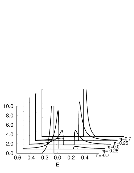
Figure 1: Effective density of states for different values of $\eta$. The free Bloch density of states is taken to be semielliptic of unit width and center of gravity at $E=0$. The hybridization is $V=0.2$ and the $f$-level $e_{f}=-0.02$

The effective dispersion $\Delta_{\vec{k}}(\eta)$ diverges for $\epsilon(\vec{k})=\eta$, i.e. when $\eta$ falls into the band region ($\min\epsilon(\vec{k})\leq\eta\leq\max\epsilon(\vec{k})$). The resulting density of states extends from $-\infty$ to $\infty$. But since $\tilde{\rho}_{0}^{(\eta)}(E)\sim\frac{1}{E^{2}}$, the respective weight vanishes. Thus, the effective width $\tilde{W}$ is very small scaling with the hybridization $V$ which must be considered for all realistic situations as a small parameter, at least very much smaller than the Coulomb interaction $U$. The “Hubbard problem” which is given by the effective Hamiltonian (22) is therefore to be ascribed to the strong coupling regime: $\frac{U}{\tilde{W}}\ggg 1$.

At this point, the advantage of the mapping onto the effective model is clear. We have replaced the periodic Anderson model, which is, though a minimal, still a two-band model with an effective single band Hubbard model, for which some standard approximation methods exist. By construction of the effective medium, the single band model turns out to belong to the strong coupling regime, thus results obtained in a $\frac{W}{U}$ perturbational theory [23] can help constructing an appropriate approximation scheme

2.3 Spectral density approach

We use a selfconsistent spectral density approach (SDA)[20, 21, 22] to find an approximate solution of the “effective” Hubbard problem defined by the Hamiltonian $\tilde{H}(\eta)$ in (22). The method is based on a physically motivated ansatz for the single-electron spectral density. Its main advantages are the physically simple concept and the non-perturbative character being not restricted to Fermi-systems but also working for Bose- and even classical systems [24, 25, 26]. Recent applications of the SDA concern the attractive ($U<0$) Hubbard model [27], the $t-J$ model [28], the magnetism and electronic structure of systems of reduced dimensions as thin films and surfaces [29, 30, 31]. It is also used for the investigation of high-$T_{c}$ superconductivity [32, 33]. In this paper we apply the SDA to the “effective medium”-Hubbard model (22).

The single-electron spectral density is defined by

$$\tilde{S}_{\vec{k},\sigma}(E)=\frac{1}{N}\Sigma_{i,j}e^{\vec{k}(\vec{R}_{i}-\vec{R}_{j})}\tilde{S}_{i,j,\sigma}(E)\\ \tilde{S}_{i,j,\sigma}(E)=\frac{1}{2\pi}\,\int\limits_{-\infty}^{+\infty}dE\,e^{-\frac{i}{\hbar}Et}\,\langle[a_{i,\sigma}(t);a_{j,\sigma}^{\dagger}(0)]_{+}\rangle$$ (30)

where $[\dots;\dots]_{+}$ denotes the anticommutator and $\langle\dots\rangle$ the thermodynamic average. The construction operators are taken to be in the Heisenberg time-dependent picture.

In an exact spectral-moment analysis in the limit $U\rightarrow\infty$, Harris and Lange have shown that the spectral density essentially consists of a two-peak structure [23]. The effective Hubbard model (22) must be considered in the strong-coupling regime. Therefore it seems appropriate to make the following ansatz for the spectral density:

$$\tilde{S}_{\vec{k},\sigma}(E)=\sum_{j=1,2}\hbar\,\tilde{\alpha}_{\vec{k},\sigma}^{(j)}\,\delta(E-\tilde{E}_{\vec{k},\sigma}^{(j)})$$ (31)

The still unknown parameters $\tilde{E}_{j,\sigma}$ and $\tilde{\alpha}_{j,\sigma}$, the quasiparticle energy and spectral weight, can be calculated by use of the first four moments of the spectral density:

$$\begin{split}\tilde{M}_{\vec{k},\sigma}^{(n)}=&\int\limits_{-\infty}^{+\infty}dE\,E^{n}\,\tilde{S}_{\vec{k},\sigma}(E)=\\ &\langle[\underbrace{[...[a_{\vec{k},\sigma},\tilde{H}]_{-},...,\tilde{H}]_{-}}_{\text{$n$-fold commutator}},a_{\vec{k},\sigma}^{\dagger}]_{+}\rangle\end{split}$$ (32)

This procedure is identical to the one performed in [22] for the real Hubbard problem. An explicit description of the calculation is presented there.

Despite its obvious restrictions, e.g. the complete neglection of quasiparticle damping, the two-pole approximation together with the moment method to calculate the free parameters is able to describe the magnetic properties of the Hubbard model surprisingly well [22, 34].

As a result one obtains a selfenergy of the following structure:

$$\tilde{\Sigma}_{\vec{k},\sigma}^{(\eta)}(E)=U\,\langle n_{i,-\sigma}^{(a)}\rangle\\ \times\frac{E-\tilde{B}_{-\sigma}-\tilde{F}_{\vec{k},-\sigma}}{E-\tilde{B}_{-\sigma}-\tilde{F}_{\vec{k},-\sigma}-U(1-\langle n_{i,-\sigma}^{(a)}\rangle)}$$ (33)

The decisive terms are $\tilde{B}_{-\sigma}$ and $\tilde{F}_{\vec{k},-\sigma}$ which distinguish this selfenergy from the Hubbard-I solution [35]. These terms, mainly consisting of higher correlation functions, may provoke a spin-dependent shift and/or deformation of the bands and may therefore be responsible for the existence of spontaneous magnetism [22, 36, 37].

The $\vec{k}$-dependent term $\tilde{F}_{\vec{k},-\sigma}$ seems to be of minor importance for the magnetic behaviour. Since $\Sigma_{\vec{k}}\tilde{F}_{\vec{k},-\sigma}=0$, it does not change the center of gravity of the density of states being mainly responsible for a deformation and narrowing of the bands. We have neglected this term in the following calculations. A detailed inspection of the influence of this term, as well as quasiparticle damping will be the subject of future investigations.

The term $\tilde{B}_{-\sigma}$ has the following structure:

$$\tilde{B}_{-\sigma}=\Delta_{0}+\frac{1}{\langle n_{i,-\sigma}^{(a)}\rangle(1-\langle n_{i,-\sigma}^{(a)}\rangle)}b_{-\sigma}\\ \begin{split}b_{-\sigma}=&\frac{1}{N}\sum_{i,j}^{i\neq j}\Delta_{i,j}\langle a_{i,-\sigma}^{\dagger}a_{j,-\sigma}(2n_{i,\sigma}^{(a)}-1)\rangle\\ =&\frac{1}{N}\int\limits_{-\infty}^{+\infty}\sum_{\vec{k}}f_{-}(E)\left(\Delta_{\vec{k}}(\eta)-\Delta_{0}\right)\\ &\left(\frac{2}{U}(E-\Delta_{\vec{k}}(\eta))-1\right)\tilde{S}_{\vec{k},\sigma}(E-\mu)\end{split}$$ (34)

$\Delta_{0}$ denotes the center of gravity of the effective electron hopping $\Delta_{i,j}$ (see equation (24)). In the case of a $\vec{k}$-independent, real selfenergy, as we have obtained with our approximation, the spectral density can be expressed as:

$$\tilde{S}_{\vec{k},\sigma}(E)=\hbar\delta\left(E-\Delta_{\vec{k}}(\eta)+\mu-\tilde{\Sigma}_{\sigma}^{(\eta)}(E)\right)$$ (35)

Together with the spectral theorem:

$$\langle n_{\sigma}^{(a)}\rangle=\frac{1}{N}\int\limits_{-\infty}^{+\infty}\sum_{\vec{k}}f_{-}(E)\tilde{S}_{\vec{k},\sigma}(E-\mu)$$ (36)

the equations (34), (33) and (35) form a closed set of equations which has to be solved selfconsistently.

After retransforming from the effective to the real medium according to equations (27) and (28) respectively, one finally obtains a solution for the periodic Anderson model.

3 Results

In the following sections, the results of the above developed theory will be presented. The system is determined by the following parameters: The free conduction band is described by a semi-elliptic density of states of the width $W=1$ and center of gravity at $E=0$, thus defining the energy scale. The $f$-level is characterized by the parameters $e_{f}$, its relative position with respect to the center of mass of the conduction band, and the on-site Coulomb interaction $U$. The hybridization $V$ is taken as a relatively small parameter, in all cases examined below, we chose $V=0.2$. Of crucial importance is the total number of electrons per lattice site, $n_{tot}=n_{f}+n_{s}$. Calculations will be made for the ground state ($T=0$) and for finite temperatures.

3.1 The paramagnetic system

In figure 2 the paramagnetic quasiparticle density of states is plotted for different values of $e_{f}$. The interaction constant is chosen to be $U=1.5$, the total occupation number is $n_{tot}=1.5$. The arrows point to the position of $\mu$, the chemical potential.

Figure 2: $s$-(dashed line) and $f$(solid line)-density of states. The parameters are $U=1.5$, $V=0.2$, $T=0$ and $n_{tot}=1.5$. The chemical potential $\mu$ is indicated by the arrows.

It can be clearly seen that the density of states is divided into three structures. With the $f$-level positioned within the free conduction band, the lower two structures exhibit band-like behavior, while the third structure, the upper “Hubbard-band” of the $f$-level, retains its atomic shape.

The gap which separates the lower two peaks, is induced by the hybridization. Its position is related to the position of the free $f$-level, and its size scales with the hybridization strength $V$.

Contrary to the upper “Hubbard-band” which is almost of pure $f$-character, these lower structures show strong mixing of $s$- and $f$-states. For $e_{f}$ approaching one of the band-edges of the free $s$-band, a strong peak of $f$-states develops.

In the example shown in figure 2, there is always a peak close to the Fermi energy. This coincidence originates from the chosen system parameters, more precisely from the number of electrons $n_{tot}$.
Due to the simple concept of the two-pole approximation used for solving the effective Hubbard model, we do not see a Kondo resonance. A Kondo resonance would strongly influence the low energy properties of the system. But as already discussed in the theory section, for describing the magnetic properties, the correct high energy behaviour of the selfenergy is of importance [37]. Therefore, we do believe in our results concerning magnetism at least for situations and temperatures where a Kondo effect is not important.

3.2 The magnetic ground state properties

In figure 3, we have drawn a magnetic phase diagram of the periodic Anderson model derived within the above developed theory. This phase diagram consists of an area where ferromagnetism is stable whereas in the remaining parameter space ($n_{tot}$ and $e_{f}$ being the variables) the ground state is paramagnetic. Antiferromagnetic ordering was not considered.

Figure 3: Magnetic phase diagram for the periodic Anderson model at $T=0$ with $U=10$ and $V=0.2$. The shaded region is ferromagnetic, the surrounding paramagnetic.

For a fixed total number of electrons $n_{tot}$ ferromagnetism can only exist if the $f$-level lies in a certain range somewhere around the lower half of the conduction band. For energetically lower positions of the $f$-level, the ferromagnetic solution of the set of equations still exists. But since the paramagnetic solution has a lower energy, the ground state is paramagnetic. With the $f$-level approaching higher energies relative to the conduction band, the number of electrons in $f$-states, $\langle n_{f}\rangle$ reduces, and the $f$-density of states broadens. It is commonly accepted that both effects reduce the stability of ferromagnetism in the system. So it is not surprising to see the system become paramagnetic with higher values of $e_{f}$.

Figure 4: $f$- and $s$-magnetization and the occupation number $n_{f}$ of the $f$-level as functions of $e_{f}$ for different total occupation numbers $n_{tot}$. ($U=10$, $V=0.2$, $T=0$)

In the following, we want to focus on the intermediate valence regime (IV) of the periodic Anderson model. Intermediate valence is characterized by non-integer values of $n_{f}$, the $f$-level occupation number. Per definitionem, an “atomic-like” level can contain either none, one or two electrons. Due to the rather high value of $U$, the local part of the Coulomb repulsion, double occupancy is suppressed. So a non-integer value of $n_{tot}$ describes mainly fluctuations between the non-occupied and the single-occupied state. The condition for IV is found for $e_{f}$ lying within the conduction band, more specific, the closer $e_{f}$ and $\mu$ are, the higher are the charge fluctuations within the $f$-states, the average $n_{f}$ occupation number is lower.

For describing rare earth materials, a total occupation number $n_{tot}$ lower than $n_{tot}=1$ is not of interest. So we will confine our investigations to the parameter range which builds up the upper right hand side of the phase diagram in figure 3. In this region, there is a “bay” in the ferromagnetic isle. For a total number of electrons around $1.75$, ferromagnetism first disappears with rising $f$-level, but reappears for little higher $f$-levels, until the system finally becomes paramagnetic again.

This is shown in more detail in figure 4, presenting the magnetization as a function of $e_{f}$ for three different electron densities $n_{tot}=\{1.5,1.6,1.7\}$. For $n_{tot}=1.7$ the two separate regions of stable ferromagnetism can be seen, but already for the lower occupation numbers, two distinct regions of ferromagnetism can be distinguished from each other.

The first of these, appearing for low values of $e_{f}$, sets in with a first order phase transition at $e_{f,\text{crit}}^{\text{lower,1}}$ and is stable up to $e_{f,\text{crit}}^{\text{upper,1}}$. The existence of a first order phase transition seems unusual. But since $e_{f,\text{crit}}^{\text{lower,1}}$ is a quantum critical point, not a thermodynamic critical point, first order phase transitions are not forbidden. At least for transitions from antiferromagnetic to paramagnetic states, first order phase transitions were experimentally observed [38].

This region, usually called Kondo regime, is characterized by almost half filled $f$-levels forming relatively large local moments. According to the Schrieffer-Wolff-transformation [16], one expects to find antiferromagnetic coupling between the $f$-moments and the conduction band moments. This behaviour is clearly seen in figure 4. But the uncorrelated conduction band shows only a weak magnetic polarization. Thus, the indirect interaction between the local moments via the conduction band is responsible for the magnetic ordering. This region of ferromagnetism could be called “local moment magnetism” (LMM), since the electrons forming the relativly large local moments are energetically far away from the Fermi energy. Thus, they do not participate in transport phenomena.

Figure 5: $f$- ($s$-) quasiparticle density of states for different values of $e_{f}$ in the upper (lower) row (full line: spin-$\uparrow$, dotted line: spin-$\downarrow$). The arrow denotes the position of the chemical potential. The total number of electrons is $n_{tot}=1.5$, the other system parameters are $V=0.2$, $T=0$, and $U=10$.

The second region of ferromagnetic ordering belongs to the intermediate valence regime of the PAM. This is specified by $f$-level occupation numbers $n_{f}$ away from half filling, and a typical broadening of the $f$-levels to bands. The average magnetic moment at each $f$-site is strongly reduced. Furthermore, the coupling between the $f$-levels and the conduction band is not always antiferromagnetic, but, depending on the system parameter, can be ferromagnetic. So, intermediate valence magnetism (IVM) is in many aspects different from the LMM.

The crossover from the LMM into the IVM regime depends on the electron density. As already mentioned, for higher $n_{tot}$, ferromagnetic order disappears at $e_{f,\text{crit}}^{\text{upper,1}}$ to reappear at $e_{f,\text{crit}}^{\text{lower,2}}$ in a second order phase transition. For $n_{tot}=1.6$, the two critical points coincide, i.e. $e_{f,\text{crit}}^{\text{upper,1}}=e_{f,\text{crit}}^{\text{lower,2}}$, thus an immediate transition between the two regions of ferromagnetism is seen. For even lower occupation numbers, e.g. $n_{tot}=1.5$ there is a crossover region with linear behaviour of the magnetization.

Figure 6: Same as figure 5, but $n_{tot}=1.6$.

Figure 7: Same as figure 5, but $n_{tot}=1.7$.

The reason for these different kinds of crossover behaviour can be found in the quasi particle densities of state (QDOS), as shown in figures 5 to 7. These QDOS correspond to the three cases presented in figure 4 with $n_{tot}=\{1.5,1.6,1.7\}$, respectively. In all three cases, the crossover region coincides with the region where the chemical potential $\mu$ crosses the hybridization gap. In case of ferromagnetism, the hybridization gap of the majority spin direction band is decisive.

For $n_{tot}=1.5$ (figure 5), the chemical potential lies in the flat region of the minority band, thus a small change of $e_{f}$ will, for constant $n_{tot}$, have only minor effects on the quasiparticle densities of states.
At $n_{tot}=1.6$ (figure 6), the different behaviour is provoked by the fact that the spin-$\downarrow$ band has a rather sharp peak around $\mu$, so already small parameter changes can have a strong impact on the system.
Finally, for $n_{tot}=1.7$ (figure 7), ferromagnetism breaks down.

It is worth to mention the possibility of a metal-insulator transition due to the hybridization gap. For $n_{tot}=1.7$, we see such a transition for $e_{f}\approx 0.1$ as the system becomes paramagnetic. On the contrary, for $n_{tot}=1.5$ or $n_{tot}=1.6$, the system stays ferromagnetic during the transition, and only spin-$\downarrow$-electrons can contribute to conductivity. But no metal-insulator transition is seen in this case.

Another fairly striking result of our calculations is the possibility of ferromagnetic coupling between the conduction band and the $f$-states.

The Schrieffer-Wolff transformation maps the PAM onto the Kondo model [16]. This model considers only a spin-exchange interaction between the conduction band and the system of $f$-levels. The effective coupling between the different electron systems is antiferromagnetic. So, one would expect to find the conduction band spin-polarized anti-parallel to the $f$-states.

As already mentioned above, we do find parameter sets, where the conduction band and the localized levels are ferromagnetically coupled. This can be seen in figure 4, and in more detail in figure 8. There, the $f$- and $s$-magnetization as well as the $f$-occupation number $n_{f}$ is plotted as a function of $n_{tot}$ for three different values of $e_{f}$ all very close to the center of gravity of the free conduction band, thus belonging to the intermediate valence regime. Dependent on $n_{tot}$ the conduction band is polarized either in the same spin direction as the $f$-system (ferromagnetic coupling), or in opposite direction (antiferromagnetic coupling). For higher $n_{f}$, the tendency is clearly towards antiferromagnetic coupling.

Figure 8: $s$- ($f$-) magnetization $m_{s}$ ($m_{f}$) and the $f$-occupation $n_{f}$ as a function of the total occupation number $n_{tot}$. In all four cases the free $f$-level $e_{f}$ is close to the center of mass of the free conduction band. The other system parameters are $U=10$, $V=0.2$ and $T=0$.

If one keeps in mind that the Schrieffer-Wolff transformation is only valid in the Kondo limit of the PAM, i.e. for half filled $f$-levels, no discrepancy is found.

The mechanism which controls the direction of spin-polarization of the conduction band can be seen in the densities of state (figures 9 to 11). While for $\rho_{f,\sigma}(E)$ the weight in each of the quasiparticle bands is distributed very asymmetric, $\rho_{s,\sigma}(E)$ is always rather flat. But due to the hybridization, the partial $s$-electron QDOS expierences the same spin-dependent bandshift as the respective $f$-QDOS. So, especially, when the lower band is not yet filled (i.e. low $n_{tot}$), the spin-$\uparrow$ $s$-band outweighs the respective spin-$\downarrow$ band. Beginning with $\mu$ crossing the upper band edge of the lower band, the spin-$\downarrow$ $s$-band gets filled, thus the QDOS induced tendency towards ferromagnetic coupling gets reduced and the antiferromagnetic exchange dominates.

Figure 9: $f$- ($s$-) quasiparticle density of states for different values of $n_{tot}$ in the upper (lower) row (full line: spin-$\uparrow$, dotted line: spin-$\downarrow$). The arrow denotes the position of $\mu$, the chemical potential. The free $f$-level is located at $e_{f}=-0.02$, the other system parameters are $V=0.2$, $T=0$, and $U=10$.

The antiferromagnetic exchange expresses itself in $\rho_{s,\sigma}(E)$ by the fact that for spin $\uparrow$ the lower of the hybridization bands has less, for spin $\downarrow$ more weight than the upper hybridization band.

Figure 10: Same as figure 9, but with $e_{f}=0.00$.

Figure 11: Same as figure 9, but with $e_{f}=0.02$.

The change of sign of the conduction band polarization provokes another interesting question. There is a dedicated set of parameters for which the $s$-band is not polarized at all, but the $f$-moments order ferromagnetically. This suggests that the spin polarization of the $s$-system is not responsible for the magnetic ordering of the $f$-levels.

In the LMM regime, the situation is clear. A strong antiferromagnetic spin exchange between localized levels and conduction band states leads to an indirect coupling of the $f$-moments, thus to ferromagntic ordering.

On the contrary, in the IVM regime, ferromagnetism in the $f$-system is obviously independent of a magnetic ordering in the conduction band. Otherwise one would expect to see some effects on the $f$-magnetization at the critical occupation number $n_{tot}$ where $m_{s}=0$. In figure 8 nothing like this can be observed. So in our opinion, spin exchange processes between the conduction band and the localized levels cannot be the major effect for producing the ferromagnetic ordering in the $f$-system. Of course, spin fluctuations are still present, thus inducing the magnetic ordering in the conduction band. But there must be a different mechanism leading to the ferromagnetic ordering of the $f$-moments. We propose a single band effect within an effective $f$-band. Due to charge fluctuations between $f$- and $s$-system, an effective $f$-$f$-hopping is possible. This leads to the formation of a narrow band analogously to a single-band Hubbard model. In the latter, ferromagnetism is, at least under certain conditions, expected to exist [39, 40, 41, 42], favored by a rather small band which should show a divergence at a band edge, and an occupation number not too far away from half filling. By examining the $f$-electron QDOS (see for example figure 9, one sees that these conditions are fullfilled in the effective $f$-band.

3.3 Finite Temperatures

When examining magnetism, the temperature dependence of several quantities is of major interest. In this section, the magnetization curves as well as the Curie-temperatures $T_{c}$ for different system parameters are presented.

When the bandwidth of the free conduction band is taken to be $W=1$, the temperatures are given in Kelvin. The figures 12 and 13 show the temperature dependence of the $s$- and $f$-magnetization for two electron densities and various $f$-level positions $e_{f}$. The $T=0$-properties for these parameters were presented in figure 4.

Figure 12: $s$- and $f$-magnetization as function of the temperature $T$ for $n_{tot}=1.5$, $U=10$ and $V=0.2$. The temperature scale is explained in the text.

Figure 13: Same as figure 12, but for $n_{tot}=1.7$. In the inset, the $f$-magnetization is shown for $e_{f}=-0.3$ (solid line) and $e_{f}=-0.2$ (dotted line).

For $n_{tot}=1.5$, as presented in figure 12, the magnetization vanishes continuously at $T_{c}$, whereas for $n_{tot}=1.7$ (see fig. 13) two different behaviours can be seen according to the two different regions of magnetism: the local moment magnetism (LMM) and the intermediate valence magnetism (IVM). For low $e_{f}$, i.e. in the LMM regime (see inset of figure 13), the phase transition is of first order, for $e_{f}$ in the IVM regime of second order. So the two distinct regions of ferromagnetism seen in figure 4 show a different temperature dependent behaviour.

In figure 12, two interesting features can be observed. There can be a temperature driven increase in $f$-magnetization, and the magnetic polarization of the conduction band can change sign as function of temperature.

A magnetization increasing with temperature seems to be quite extraordinary, and at first sight, unplausible for thermodynamic reasons. But on second sight, even a temperature-driven spontaneous ordering from a paramagnetic to a ferromagnetic state is possible [43]. In our case, the system does not undergo a phase transition, only the magnetization increases slightly for certain parameters. This can be easily understood as a quasiparticle densities of states effect: If the system parameters are chosen, such that the lower edge of the upper hybridization spin $\uparrow$-band is close to, but still above the Fermi energy, these states are unoccupied for $T=0$. But already a small softening of the Fermi function can induce a strong increase in occupied spin-$\uparrow$ states since this band edge generically consists of a rather sharp peak. The ratio of spin-$\uparrow$ electrons to spin-$\downarrow$ electrons increases, the magnetization rises.

The other feature is observed in the lower picture of figure 12 showing the conduction band polarization. As already seen for $T=0$, it can either be parallel (ferromagnetic coupling) or antiparallel (antiferromagnetic coupling) to the $f$-magnetization, but sometimes, e.g. for $e_{f}=-0.05$, it can also cross the $m_{s}=0$-axis at some temperature $T^{\star}$. Quite remarkable is the behaviour of the $f$-magnetization which is continuous even at $T=T^{\star}$. This resembles the $T=0$ behaviour of the magnetization as function of $n_{tot}$ in the IV regime discussed in the previous section. Again, it is indicated that the coupling mechanism responsible for the alignment of the $f$-moments in the intermediate valence regime does not depend on the explicit polarization of the conduction band. This polarization has to be understood as a consequence, and not the cause of the ordering of the $f$-system.

Figure 14: $f$-electron quasiparticle density of state (QDOS) as a function of energy for different temperatures (solid line: spin $\uparrow$, dashed line: spin $\downarrow$). The system parameters are $n_{tot}=1.7$, $e_{f}=-0.2$, $U=10$ and $V=0.2$. The corresponding magnetization curve is presented in the inset of figure 13. The system shows a first order phase transition at $T_{c}\approx 208$.

In the figures 14 and 15, the demagnetization behaviour is examined by means of the quasi particle densities of states. These illustrate both the first order transition in the LMM regime ($e_{f}=-0.2$: figure 14) and the second order transition in the IV region ($e_{f}=-0.05$: figure 15). In both cases, the demagnetization is characterized by two effects, a bandshift and a weight transfer mechanism. The bandshift between spin $\uparrow$ and spin $\downarrow$ band decreases with increasing temperature while at the same time a transfer of spectral weight between the hybridization bands occurs. For the spin $\uparrow$-bands, weight is transferred from the lower to the upper band, for the spin $\downarrow$-bands just the contrary takes place.

For $e_{f}=-0.2$, ferromagnetism breaks down at $T=T_{c}\approx 208$, we see a first order phase transition. Contrarily, for $e_{f}=-0.05$, the demagntization behaves smoothly up to $T=T_{c}\approx 114$, thus a second order phase transition occurs.

Figure 15: same as figure 14, but for $e_{f}=-0.05$. This corresponds to the dashed line in figure 13, with $T_{c}\approx 114$.

Finally, in figure 16, the Curie-temperatures as function of $n_{tot}$ (upper figure) and $e_{f}$ (lower figure) are presented. The continuous vanishing of $T_{c}$ as a function of $n_{tot}$ corresponds to the second order phase transitions seen in figure 8.

Comparing figure 8 and the Curie temperature as a function of $n_{tot}$ in the IV regime (figure 16), one observes that the maximum of $T_{c}(n_{tot})$ coincides neither with the maximum of $m_{f}(n_{tot})$ not the maximum of $m_{s}$ at $T=0$. Taking the Curie temperature as a measure of the thermodynamic stability of ferromagnetism, this indicates again that the magnetic polarization of the conduction band does not directly cause the magnetic ordering of the $f$-moments. Thus, we conclude that the magnetic polarization of the conduction band is rather induced by the magnetically ordered atomic levels than responsible for the ordering itself. This supports our proposition that the magnetic ordering of the $f$-moments in the intermediate valence regime is rather a single band effect within the $f$-system than caused by a spin-exchange between $f$-levels and conduction band.

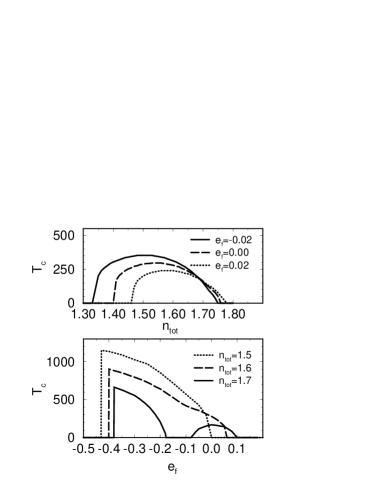
Figure 16: Curie-temperature $T_{c}$ in the upper picture, as function of $n_{tot}$, and in the lower as function of $e_{f}$ ($U=10$ and $V=0.2$)

In figure 16 showing $T_{c}$ as a function of $e_{f}$, the splitting of the two regions of ferromagnetism for $n_{tot}\gtrapprox 1.7$ can be seen again. The lowest boundary of ferromagnetism with respect to $e_{f}$ is given by the first order phase transition at the quantum critical point $e_{f,\text{crit}}^{\text{lower},1}$. Right above this critical point, both the Curie temperature as well as $m_{f}(T=0)$ show their maximum. Here, in the LMM regime, the Schrieffer-Wolff transformation suggests that an effective coupling of $f$-moments is possible only via an (antiferro-) magnetic exchange with the conduction band. But again, for the IVM region, no connection can be made between the $T=0$ moments of the two electronic subsystems and the Curie temperature $T_{c}$.

4 Conclusions

In this paper, we have presented a new approach to the periodic Anderson model. Our approximation is based on an exact mapping of the PAM onto an effective Hubbard model. Since this effective model is clearly located in the strong coupling regime, a for this limit rather well motivated approximation,the SDA is used to find self-consistent solutions. Even though the particular low-temperature properties of the Anderson model like a formation of a Kondo resonance are not accessible within our approximation, it is trustworthy concerning magnetism. A major advantage of this approach is its numerical simplicity, enabling calculations for the full parameter range and the accessibility of all major quantities of interest via the selfenergy given on the real axis.

Using this method we have shown the $T=0$ phase diagram and have found two distinct regions of ferromagnetism. The first of these is best described by the term “local moment magnetism” (LMM) while the other located within the intermediate valence region (IVM) displays itinerant character.

The local moment region is close to the Kondo regime of the PAM. The magnetic moments within the $f$-system are fully polarized, the coupling between $f$-moments and conduction band is antiferromagnetic, as expected from the Schrieffer-Wolff transformation. The Curie temperatures are rather high.

On the other side, the magnetism in the intermediate valence regime is quite weak, in a sense that the average magnetic moment per site is low and the Curie temperatures are smaller than in the LMM region. The magnetic polarization of the conduction band can either be parallel or antiparallel to the $f$-moments, at some isolated points, the conduction band is not polarized at all. This means, the polarization of the conduction band should be of minor importance to the magnetic ordering of the $f$-moments.

We conclude that the mechanism resposible for the ferromagnetic ordering is different for the LMM and the IVM regime. Whereas in the LMM regime, a spin-exchange according to the Schrieffer-Wolff transformation causes ferromagnetic ordering of the $f$-moments, in the IV regime, the spin fluctuations still lead to a spin polarization of the conduction band, but rather more important for the ferromagnetic ordering in the $f$-levels are the charge fluctuations leading to an effective broadening of the $f$-levels to a band. This band has those properties expected to form ferromagnetism within a single-band Hubbard model.

References

- [1] N. Grewe and F. Steglich, Handbook on the Physics and Chemistry of Rare Earth 14, 343 1991.
- [2] P. Hill, F. Willis, and N. Ali, J. Phys.: Condens. Matter 4, 5015 1992.
- [3] T. Burghadt, E. Hallmann, and A. Eichler, Physica B 230-232, 214 1997.
- [4] P. W. Anderson, Phys. Rev. 124(1), 41 1961.
- [5] T. Pruschke and N. Grewe, Z. Phys. B 74, 439 1989.
- [6] T. Pruschke, D. L. Cox, and M. Jarrell, Phys. Rev. B 47(7), 3553 1993.
- [7] A. M. Tsvelick and P. B. Wiegmann, Advances in Physics 32(4), 453 1983.
- [8] H.J. Leder and B. Mühlschlegel, Z. Phys. B 29, 341 1978.
- [9] E. Halvorsen and G. Czycholl, J. Phys.: Condens. Matter 8, 1775 1996.
- [10] T. Venkatappa Rao, G. Gangadhar Reddy, and A. Ramakanth, Solid State Commun. 81(9), 795 1992.
- [11] T. Venkatappa Rao, G. Gangadhar Reddy, and A. Ramakanth, J. Phys. Chem. Solids 55(2), 175 1994.
- [12] N. Grewe, T. Pruschke, and H. Keiter, Z. Phys. B 71, 75 1988.
- [13] N. Grewe, Solid State Commun. 66(10), 1053 1988.
- [14] A. Georges, G. Kotliar, W. Krauth, and M. J. Rozenberg, Rev. Mod. Phys. 68(1), 13 January 1996.
- [15] A.N. Tahvildar-Zadeh, M. Jarrell, and J.K. Freericks, Phys. Rev. B 55(6), R3332 1997.
- [16] J. R. Schrieffer and P. A. Wolff, Phys. Rev. 149(2), 491 1966.
- [17] D. Malterre, M. Grioni, and Y. Baer, Adv. Phys. 45(4), 299 1996.
- [18] S. Hüfner, Ann. Phys. 5, 453 1996.
- [19] A.J. Arko et al, Physica B 230-232, 16 1997.
- [20] W. Nolting, Phys. Lett. 38A, 417 1972.
- [21] W. Nolting and W. Borgieł, Phys. Rev. B 39(10), 6962 1989.
- [22] T. Herrmann and W. Nolting, J. Magn. Mat. 170, 253 1997.
- [23] A. Harris and R. Lange, Phys. Rev. 157(2), 295 1967.
- [24] W. Nolting and A. M. Oles, Physica 143A, 296 1983.
- [25] Campana et al, Physica 123A, 279 1984.
- [26] L.A.B. Benandes et al, phys.stat.sol.(b) 135, 581 1986.
- [27] T. Schneider, M. H. Pederson, and J. J. Rodriguez-Nunez, Z.Phys. B 100, 263 1996.
- [28] M. Maske, Phys.Rev.B 48, 1160 1993.
- [29] M. Potthoff and W. Nolting, J. Phys.: Condens. Matter 8, 4937 1996.
- [30] M. Potthoff and W. Nolting, Surf. Sci. 377-379, 457 1997.
- [31] M. Potthoff and W. Nolting, Phys. Rev. B 55, 2741 1997.
- [32] J. Beenen and D. M. Edwards, Phys. Rev. B 52(18), 13636 1995.
- [33] B. Mehlig, H. Eskes, R. Hayn, and M.B.J. Meinders, Phys. Rev. B 52(4), 2463 1995.
- [34] T. Herrmann and W. Nolting, Solid State Commun. 103(6), 351 1997.
- [35] J. Hubbard, Proc. R. Soc. London, Ser. A 276, 238 1963.
- [36] M. Potthoff, T. Wegner, and W. Nolting, Phys. Rev. B 55(24), 55 97.
- [37] M. Potthoff, T. Herrmann, T. Wegner, and W. Nolting, to be published 1998.
- [38] F. Steglich et al, Physica B 223&224, 1 1996.
- [39] M. Ulmke, Eur. Phys. J. B 1, 301 1998.
- [40] H. Tasaki, preprint cond-mat/9712219.
- [41] J. Wahle et al, preprint cond-mat/9711242 1997.
- [42] D. Vollhardt et. al., preprint cond-mat/9701150 1997.
- [43] S. V. Vonsovsky, Yu. P. Irkhin, V. Yu. Irkhin, and M. I. Katsnelson, Journal de Physique C8, 253 1988.