Exact Eigenstates of Tight-Binding Hamiltonians on the Penrose Tiling

Abstract

We investigate exact eigenstates of tight-binding models on the planar rhombic Penrose tiling. We consider a vertex model with hopping along the edges and the diagonals of the rhombi. For the wave functions, we employ an ansatz, first introduced by Sutherland, which is based on the arrow decoration that encodes the matching rules of the tiling. Exact eigenstates are constructed for particular values of the hopping parameters and the eigenenergy. By a generalized ansatz that exploits the inflation symmetry of the tiling, we show that the corresponding eigenenergies are infinitely degenerate. Generalizations and applications to other systems are outlined.

I Introduction

The discovery of quasicrystals by Shechtman et al. [1] stimulated wide interest in the physics of these materials which are intermediate between periodic and random structures. Besides icosahedral quasicrystals, which are aperiodic in all three dimensions of space, also periodically layered structures with planar quasiperiodic order and non-crystallographic rotational symmetries were found, comprising dodecagonal,[2] decagonal,[3] and octagonal [4] phases with twelve-, ten-, and eightfold symmetry, respectively. Although the fundamental question “where are the atoms?”, raised e.g. in Ref. [5], has only been answered partially to date, most structure models of quasicrystals are based on two- or three-dimensional quasiperiodic tilings or their disordered versions (random tilings).

An important and exciting problem in condensed-matter physics is whether the quasiperiodic structure leads to new and unexpected physical properties. In particular transport properties, as for instance electric or heat conductance, are strongly effected by the non-periodic order. Indeed, many quasicrystalline alloys are characterized by very high values of electric resistivity, by a negative temperature coefficient of resistivity, and by a low electronic contribution to the specific heat which points to a small density of states at the Fermi energy. It is difficult to explain these striking features, because a rigorous theory of the electronic structure of quasiperiodic materials does not exist. For want of a simple analogy of Bloch theory for quasicrystals, one either carries out numerical calculations for as large clusters as possible, or one tries to make exact statements about the electronic wave functions in simple models.

We consider tight-binding models on the two-dimensional rhombic Penrose tiling.[6] Our models are so-called vertex models because we locate the atoms at the vertices of the tiling. Interactions are taken into account only between neighboring vertices connected by edges or by diagonals of the rhombi. In our calculations, we restrict ourselves to a single $s$-type atomic orbital per vertex. This makes the transfer integrals $t_{ij}$ independent of the angular orientation and leads to the following Hamiltonian

$$H\;=\;\sum_{i}|i\rangle\,\varepsilon_{i}\,\langle i|\;+\;\sum\limits_{i,j}|i\rangle\,t_{ij}\,\langle j|$$ (1)

where $|i\rangle$ denotes a Wannier state localized at vertex $i$, and $\varepsilon_{i}$ are on-site energies. For the hopping integrals $t_{ij}$, we choose five different values $1$, $d_{1}$, $d_{2}$, $d_{3}$, $d_{4}$, depending on the distance of the vertices $i$ and $j$, see Fig. 1. Here, $t_{ij}=1$ for vertices connected by an edge of the tiling, $t_{ij}=d_{1}$ ($d_{2}$) for the long (short) diagonal of the ‘fat’ rhombus, and $t_{ij}=d_{3}$ ($d_{4}$) for the long (short) diagonal of the ‘thin’ rhombus, respectively.

As the Penrose tiling is arguably the most popular among the quasiperiodic tilings, it is not surprising that tight-binding models defined on the Penrose tiling have been investigated rather thoroughly. Besides the vertex model,[7, 8, 9, 10, 11, 12, 13, 14, 15, 16, 17, 18, 19] the so-called center model was considered,[20, 21, 22, 23, 24] where atoms are located in the center of the rhombi, and hopping may occur between adjacent tiles — this is nothing but a vertex model on the dual graph of the Penrose tiling. However, most results rely on numerical approaches, and only few exact results on the spectrum of the tight-binding Hamiltonian are known. In particular, so-called ‘confined states’ have been investigated in detail, both for the vertex [9, 14] and the center model.[22] These are infinitely degenerate, strictly localized eigenstates corresponding to a particular value of the energy, which occur as a consequence of the local topology of the tiling, see also Ref. [18]. Furthermore, for a Hamiltonian (1) with particular on-site energies $\varepsilon_{i}$ chosen according to the vertex type at site $i$, the exact self-similar ground state could be constructed.[10] Based on the same idea, several non-normalizable eigenstates of the center model and their multifractal properties were obtained exactly.[23] These solutions, restricted to special values of the hopping integrals, were derived from a suitable ansatz for the eigenfunctions. According to this ansatz, the wave function at a site depends only on its neighborhood and on a certain integer number associated to the site, a ‘potential’, which is derived from the matching rules of the Penrose tiling.[10]

In this paper, we apply the same ansatz to the vertex model on the Penrose tiling. The solution is more complicated than for the center model, where the coordination number (i.e., the number of neighbors) is always equal to four, whereas for the vertex model it varies between three and seven, or between six and fourteen if we include neighbors along diagonals, respectively. For suitably chosen transfer integrals, we derive exact eigenstates of the Hamiltonian (1) and analyze their multifractal behavior. As observed for the center model,[23] we find that these states are infinitely degenerate, i.e., for fixed value of the energy the eigenfunctions still involve one free parameter. In order to show this, we need to generalize the ansatz exploiting the inflation symmetry of the Penrose tiling.

Our paper is organized as follows. In the subsequent section, we discuss the labeling of the rhombi with two kind of arrows and the associated potentials. In Sec. III, we introduce the ansatz for the wave function and solve the tight-binding equations for two cases, the first one with $\varepsilon_{i}=0$ and $d_{i}\neq 0$, and the second one with $d_{i}=0$ but various on-site energies. A generalized ansatz, based on the inflation symmetry of the tiling, is considered in Sec. IV. In Sec. V, we perform a fractal analysis of the wave functions, i.e., we calculate the generalized dimensions. Finally, we conclude in Sec. VI.

II Edge-labeling and Potentials

Following de Bruijn,[25] we mark the rhombi with single and double arrows as shown in Fig. 2. The matching rules require that arrows on adjacent edges match. Fixing a certain site $O$ as the origin, we assign to a site $i$ two integers $n(i)$ and $m(i)$ which count the number of single and double arrows, respectively, along an arbitrary path connecting the origin $O$ and site $i$. This is well-defined because, along any closed path, the total number of single and double arrows vanishes, as can be seen from Fig. 2. We refer to these integers $n(i)$ and $m(i)$ as ‘potentials’ at site $i$ because they are integrals of the two vector fields defined by the arrows. The distributions of the potentials are rather irregular and show the following properties:

• The single-arrow potential $n(i)$ is directly related to the sum $t(i)\in\{1,2,3,4\}$ of the five-dimensional indices denoting the translation class of the site $i$. It takes only two values: $n(i)=0$ if $t(i)\in\{2,3\}$ and $n(i)=1$ if $t(i)\in\{1,4\}$ (provided the origin has translation class $t(O)\in\{2,3\}$).

• The double-arrow potential $m(i)$ is unbounded. Its distribution on a finite patch is shown in Fig. 3. For a detailed discussion of the distribution, see Ref. [10].

The potential $m(i)$ is the key ingredient in the construction of exact eigenfunctions of tight-binding Hamiltonians on the Penrose tiling.

III Solutions of the tight-binding equations

We want to construct solutions of the tight-binding equations

$$\sum_{j}t_{ij}\,\phi_{j}\;=\;(E-\varepsilon_{i})\>\phi_{i}\;,$$ (2)

where we sum over all neighbors $j$ of the site $i$. As an ansatz, we demand that the wave function amplitude $\phi_{i}$ at site $i$ depends solely on the vertex type $\nu(i)\in\{1,2,\ldots,8\}$ and on the potential $m(i)$. This leads to the following ansatz

$$\phi_{i}\;=\;A_{\nu(i)}\,\beta^{\,m(i)}\;.$$ (3)

The eight vertex types of the Penrose tiling are shown in the top row of Fig. 4. The corresponding eight amplitudes $A_{\nu}$ and $\beta$ are parameters.

A The case $\varepsilon_{i}=0$

For simplicity, we first concentrate on the case with on-site energies $\varepsilon_{i}=0$. With the ansatz (3), the infinite set of equations (2) reduces to a finite set comprising as many equations as there are second-order vertex types in the tiling. By a second-order vertex type we mean the neighborhood of a site up to its second coordination zone. There are 31 different second-order vertex types in the Penrose tiling, these are shown in Fig. 4, grouped together according to the first-order vertex type of the central site given in the top row. Thus, we have $31$ linear equations in the 14 variables $A_{\nu}$ ($\nu=1,\ldots,8$), $\beta$, $d_{1}$, $d_{2}$, $d_{3}$, $d_{4}$, and $E$. As it is straightforward to derive the equations from the second-order vertex types of Fig. 4, we refrain from listing them here. Instead, we consider as an example only the second-order vertex types in the first column of Fig. 4, which we show again in Fig. 5 (rotated by 90 degrees) together with the corresponding values of the potential $m(i)$. This yields the following four equations

$$EA_{1} = d_{4}A_{3}\beta+2(A_{2}+A_{3})+d_{1}(A_{2}+A_{5}+A_{7})\beta^{-1}$$ (4)

$$= d_{4}A_{3}\beta+2(A_{2}+A_{3})+d_{1}(A_{2}+A_{5}+A_{5})\beta^{-1}$$ (5)

$$= d_{4}A_{3}\beta+2(A_{2}+A_{3})+d_{1}(A_{2}+A_{7}+A_{5})\beta^{-1}$$ (6)

$$= d_{4}A_{3}\beta+2(A_{2}+A_{3})+d_{1}(A_{2}+A_{7}+A_{7})\beta^{-1}$$ (7)

two of which (the first and the third) are identical because the corresponding patterns are mirror images of each other.

At first sight, as the number of variables, $14$, is much smaller than the number of equations, $31$, one might expect that only the trivial solution ($\phi_{i}\equiv 0$) exists. However, this is not the case, for suitably chosen values of the hopping parameters $d_{1}$, $d_{2}$, $d_{3}$, $d_{4}$, and the energy $E$, non-trivial solutions exist, because the equations are not independent. To see this, note that the second-order vertex types within one column of Fig. 4 differ only slightly from each other, which means that the corresponding equations are also very similar as can be seen in the example (LABEL:eq:system_of_equations). Thus, they can be substantially simplified by subtraction. For example, the differences between the equations in (LABEL:eq:system_of_equations) result in the single equation

$$d_{1}(A_{5}-A_{7})\;=\;0$$ (9)

which implies $A_{5}=A_{7}$ (unless $d_{1}$ vanishes). From the analogous equations for the other vertex types, it turns out that the amplitudes $A_{\nu(i)}$ depend only on the translation class $t(i)$ of the site $i$, rather than on its specific vertex type $\nu(i)$. This means

$$A_{1}\,=\,A_{4}\,=\,A_{6}\qquad(t\in\{1,4\})$$ (10)

$$A_{2}\,=\,A_{3}\,=\,A_{5}\,=\,A_{7}\,=\,A_{8}\qquad(t\in\{2,3\})\;.$$ (11)

With this, all equations corresponding to second-order vertex types with the same central vertex reduce to a single equation, and one is left with the following eight equations

$$EA_{1} = d_{4}A_{2}\beta+4A_{2}+3d_{1}A_{2}\beta^{-1}$$ (12)

$$= 5A_{2}+5d_{1}A_{2}\beta^{-1}$$ (13)

$$= 2d_{4}A_{2}\beta+3A_{2}+d_{1}A_{2}\beta^{-1}$$ (14)

$$EA_{2} = (d_{1}A_{1}+2A_{2})\beta+2A_{1}+2(d_{2}+d_{3})A_{2}+A_{2}\beta^{-1}$$ (15)

$$= A_{1}+2d_{2}A_{2}+(2A_{2}+d_{4}A_{1})\beta^{-1}$$ (16)

$$= (3d_{1}A_{1}+5A_{2})\beta+2A_{1}+4d_{3}A_{2}$$ (17)

$$= (4d_{1}A_{1}+5A_{2})\beta+A_{1}+2d_{3}A_{2}$$ (18)

$$= (5d_{1}A_{1}+5A_{2})\beta$$ (19)

for central vertices of type $1$, $4$, $6$, and $2$, $3$, $5$, $7$, $8$, respectively.

For this system of equations, we obtain three sets of non-trivial solutions, expressed in terms of the parameter $\beta$ which may be chosen freely. Here, we introduce

$$b_{\pm}\;:=\;\frac{1}{\beta\pm\beta^{-1}}$$ (20)

to abbreviate the formulae below.
Solution (1): The wave function has the form

$$\phi_{i}\;=\;\left\{\begin{array}[]{ll}(1-2\beta^{2})\beta^{\,m(i)}&\mbox{for $t(i)\in\{1,4\}$}\\ \beta^{\,m(i)+1}&\mbox{for $t(i)\in\{2,3\}$}\end{array}\right.$$ (21)

for transfer integrals and energy given by

$$d_{1}=\frac{1}{2}b_{-} d_{2}=-\frac{3}{4}b_{-}+b_{-}^{-1}$$ (22)

$$d_{3}=-\frac{1}{4}b_{-}+\frac{1}{2}b_{-}^{-1} d_{4}=b_{-}$$ (23)

$$E\,=-\frac{5}{2}b_{-}$$ (24)

Solution (2): Here,

$$\phi_{i}\;=\;\left\{\begin{array}[]{ll}\beta^{\,m(i)+1}&\mbox{for $t(i)\in\{1,4\}$}\\ \beta^{\,m(i)}&\mbox{for $t(i)\in\{2,3\}$}\end{array}\right.$$ (25)

with

$$d_{1}=-b_{+} d_{2}=\frac{3}{2}b_{+}-\frac{1}{2}b_{+}^{-1}$$ (26)

$$d_{3}=-(\frac{1}{2}+\beta^{2})b_{+} d_{4}=(1-\beta^{-2})b_{+}$$ (27)

$$E\,=5b_{+}$$ (28)

Solution (3): Finally,

$$\phi_{i}\;=\;\left\{\begin{array}[]{ll}\beta^{\,m(i)}&\mbox{for $t(i)\in\{1,4\}$}\\ \beta^{\,m(i)+1}&\mbox{for $t(i)\in\{2,3\}$}\end{array}\right.$$ (29)

where

$$d_{1}=-(\frac{1}{2}+\beta^{2})b_{+} d_{2}=\frac{1}{4}b_{+}-\frac{1}{2}b_{+}^{-1}$$ (30)

$$d_{3}=-(\frac{1}{4}+\beta^{-2})b_{+} d_{4}=-b_{+}$$ (31)

$$E\,=\frac{5}{2}b_{+}$$ (32)

For each of these solutions, there exists an additional solution for a slightly generalized ansatz

$$\tilde{\phi}_{i}=\tilde{A}_{\nu(i),t(i)}\>\tilde{\beta}^{\,m(i)}$$ (33)

that involves the translation class $t(i)$ at site $i$. Note that for each vertex type there are only two possible values, $t(i)\in\{1,4\}$ for $\nu(i)\in\{1,4,6\}$ and $t(i)\in\{2,3\}$ for $\nu(i)\in\{2,3,5,7,8\}$, which were not distinguished in our previous ansatz, see Eq. (11). The wave functions differ from the solutions given in Eqs. (21), (25), and (29) only by an alternating sign which depends on the translation class

$$\tilde{\phi}_{i}=(-1)^{t(i)}\phi_{i}$$ (34)

and by a sign change in the parameters, i.e., $\tilde{d_{1}}=-d_{1}$, $\tilde{d_{2}}=-d_{2}$, $\tilde{d_{3}}=-d_{3}$, $\tilde{d_{4}}=-d_{4}$, and $\tilde{E}=-E$. Note that the two models differing by this sign change are not trivially related, because the hopping parameter along the edges of the tiles does not change its sign — it is always equal to $1$. These six solutions exhaust all non-trivial solutions in terms of the ansatz (33), but we note that for a given set of hopping parameters, i.e., for a given Hamiltonian, this yields at most one single solution. Some examples of the wave functions (21) for different values of $\beta$ are presented in Fig. 6.

B The case $\varepsilon_{i}\neq 0$

In order to obtain the eigenstates described above, we introduced parameters in the Hamiltonian (1) and determined them by requiring that the ansatz (3) fulfills the tight-binding equations (2). In Eq. (1), we already included the possibility of site-dependent on-site energies $\varepsilon_{i}$. In the present case, it is natural to choose the on-site energies $\varepsilon_{i}$ according to the vertex type of site $i$. That is, $\varepsilon_{i}=\mu_{\nu(i)}$ with eight parameters $\mu_{1},\ldots,\mu_{8}$ according to the eight vertex types of the Penrose tiling.

Of course, we can perform the same analysis as above for the more general problem — it just amounts to replacing the left-hand side of the first three lines of Eqs. (19) by $(E-\mu_{\nu})A_{1}$ with $\nu=1,4,6$, and in the remaining five lines by $(E-\mu_{\nu})A_{2}$ with $\nu=2,3,5,7,8$, respectively. We do not show the explicit solution of the full problem because it is rather lengthy. Although the general solution contains a few free parameters, for a given Hamiltonian we still find at most one exact eigenstate.

In order to compare with Sutherland’s result,[10] we consider the case without hopping along the diagonals of the rhombi, i.e., $d_{1}=d_{2}=d_{3}=d_{4}=0$. We can express the solutions in terms of the three parameters $E$, $\beta$, and $\gamma:=A_{2}/A_{1}$:

$$\makebox[123.0pt][l]{$\displaystyle\mu_{1}=E-4\gamma$}\mu_{2}=E-2\beta-\beta^{-1}-2\gamma^{-1}$$ (35)

$$\makebox[123.0pt][l]{$\displaystyle\mu_{3}=E-2\beta^{-1}-\gamma^{-1}$}\mu_{4}=E-5\gamma$$ (36)

$$\makebox[123.0pt][l]{$\displaystyle\mu_{5}=E-5\beta-2\gamma^{-1}$}\mu_{6}=E-3\gamma$$ (37)

$$\makebox[123.0pt][l]{$\displaystyle\mu_{7}=E-5\beta-\gamma^{-1}$}\mu_{8}=E-5\beta$$ (38)

Setting $\gamma=1$ one recovers Sutherland’s solution.[10]

Taking into account that we have introduced eight parameters $\mu_{\nu}$ in our the Hamiltonian, it was almost obvious that solutions exist. It would be, however, more interesting to introduce additional parameters in the ansatz for the wave function. In this way, one might perhaps be able to obtain several eigenstates of a given Hamiltonian and thus come closer to the general solution of our problem. This is the subject of the following section.

IV Generalized ansatz for the eigenfunctions

The Penrose tiling possesses a so-called inflation/deflation symmetry.[6, 10] In an inflation step, the two types of rhombi are dissected into smaller pieces that again constitute a rhombic Penrose tiling, but on a smaller scale with all lengths divided by the golden ratio $\tau=(1+\sqrt{5})/2$. The inverse procedure, in which tiles are combined to form larger tiles, is known as deflation.

The idea now is to generalize the ansatz (3) for the wave function by using the vertex types and potentials of the deflated tiling in addition to those of the original tiling. Even more general, one may consider a sequence of $n$ tilings obtained by successive deflation steps, probing the original tiling on larger and larger length scales. In this way, we assign to each vertex $i$ of the original tiling a sequence of integers $\{\nu_{k}(i)\}$, $k=0,1,\ldots,n$, where $\nu_{k}(i)$ specifies the corresponding vertex type in the $k$-fold deflated tiling, with $k=0$ referring to the original tiling. This leads to the following generalized ansatz for the wave function

$$\phi_{i}^{[n]}\;=\;A_{\{\nu_{k}(i)\}}\>\prod_{k=0}^{n}\beta_{k}^{\,m_{k}(i)}$$ (39)

where $m_{k}$ denotes the double-arrow potential in the $k$-fold deflated tiling, and $\beta_{k}$ are $n+1$ free parameters.

It is not completely obvious how to assign the vertex type $\nu_{k}(i)$ of a site $i$ in the $k$-fold deflated tiling. Here, we decided to use the concept of the Voronoi cell. We are looking for a Voronoi cell of the deflated tiling that covers the Voronoi cell of our site $i$ in the original tiling completely, or at least its largest part. In Fig. 7, we show how the Voronoi cells of the original and the two-fold deflated tiling relate to each other. If a cell of the original tiling is shared between several larger cells, we assign the vertex to the cell with the maximum overlap. However, there are still ambiguities when overlaps of equal area occur. For instance, let us concentrate on the case $n=2$. In the example shown in Fig. 8, one recognizes that the cell corresponding to vertex type $1$ (cf. Fig. 4) may be dissected equally between the cells corresponding to vertex types $2$ or $3$ of the deflated tiling. In this case, we cannot assign the deflated vertex type unequivocally. Therefore, we demand that the corresponding terms in the ansatz (39) are equal. In our example, this yields the equation $A_{221}=A_{321}$ for the amplitudes $A_{\nu_{2}\nu_{1}\nu_{0}}$ in the ansatz (39), labeled by three digits according to the three vertex types. Considering also the first deflation step, not shown in Fig. 7, one finds another condition $A_{222}=A_{232}$.

We now use the ansatz (39) to find solutions of the tight-binding equations. Here, we restrict ourselves to the case $n=2$. In order to set up the equations, we need to consider larger patches which may be obtained by two-fold inflation of the $31$ second-order vertex types of Fig. 4. Each of these patches then leads to a number of equations. Of the $8^{3}$ possible combinations of indices $\nu_{2},\nu_{1},\nu_{0}$, only $25$ occur in the Penrose tiling. Altogether we have to deal with a system of $97$ equations in 32 variables, namely $25$ amplitudes $A_{\nu_{2}\nu_{1}\nu_{0}}$, three variables $\beta_{2}$, $\beta_{1}$, $\beta_{0}$, the four hopping parameters $d_{1}$, $d_{2}$, $d_{3}$, $d_{4}$, and the energy $E$. We used Mathematica[26] to solve this system. As above, we find three sets of solutions, which we express in terms of $\beta_{20}:=\beta_{2}\beta_{0}$ and $\beta_{1}$. They have the following form.
Solution (1’): The $25$ amplitudes, without normalization, are

$$A_{221}=A_{321}=-\beta_{20}\,(2\beta_{20}^{2}-\beta_{1}^{2})\,\beta_{0}$$ (40)

$$A_{222}=A_{322}=A_{232}=A_{532}=A_{732}=A_{832}=\beta_{20}^{2}\,\beta_{1}\,\beta_{0}$$ (41)

$$A_{233}=A_{333}=\beta_{20}^{2}\,\beta_{0}$$ (42)

$$A_{123}=A_{423}=A_{623}=A_{133}=A_{633}=\beta_{20}^{3}$$ (43)

$$A_{654}=A_{174}=A_{484}=-\beta_{20}^{2}\,(2\beta_{20}^{2}-\beta_{1}^{2})$$ (44)

$$A_{365}=A_{217}=A_{548}=A_{748}=A_{848}=\beta_{20}\,\beta_{1}^{2}\,\beta_{0}^{2}$$ (45)

$$A_{236}=A_{336}=-(2\beta_{20}^{2}-\beta_{1}^{2})\,\beta_{0}^{2}$$ (46)

and the transfer integrals and the energy are given by the same expressions (24) as for solution (1), where now

$$b_{\pm}\;:=\;\frac{\beta_{20}\,\beta_{1}}{\beta_{20}^{2}\pm\beta_{1}^{2}}\;.$$ (47)

In contrast to the amplitudes, the transfer integrals and the energy are hence expressed exclusively in terms of $\beta_{20}$ and $\beta_{1}$, that is, the hopping parameters and the energy depend on $\beta_{2}$ and $\beta_{0}$ only via the product $\beta_{20}$.
Solution (2’): Here, the amplitudes read

$$A_{221}=A_{321}=\beta_{20}^{2}\,\beta_{0}$$ (48)

$$A_{222}=A_{322}=A_{232}=A_{532}=A_{732}=A_{832}=\beta_{20}\,\beta_{1}\,\beta_{0}$$ (49)

$$A_{233}=A_{333}=\beta_{20}\,\beta_{0}$$ (50)

$$A_{123}=A_{423}=A_{623}=A_{133}=A_{633}=\beta_{20}^{2}$$ (51)

$$A_{654}=A_{174}=A_{484}=\beta_{20}^{3}$$ (52)

$$A_{365}=A_{217}=A_{548}=A_{748}=A_{848}=\beta_{1}^{2}\,\beta_{0}^{2}$$ (53)

$$A_{236}=A_{336}=\beta_{20}\,\beta_{0}^{2}$$ (54)

and the parameters now follow from the expressions (28) for solution (2) with $b_{+}$ given by Eq. (47) and

$$\beta\;:=\;\frac{\beta_{20}^{2}}{\beta_{1}^{2}}\;;$$ (55)

thus again they depend on $\beta_{0}$ and $\beta_{2}$ only via $\beta_{20}$.
Solution (3’): Finally,

$$A_{221}=A_{321}=\beta_{20}\,\beta_{1}^{2}\,\beta_{0}$$ (56)

$$A_{222}=A_{322}=A_{232}=A_{532}=A_{732}=A_{832}=\beta_{20}^{2}\,\beta_{1}\,\beta_{0}$$ (57)

$$A_{233}=A_{333}=\beta_{20}^{2}\,\beta_{0}$$ (58)

$$A_{123}=A_{423}=A_{623}=A_{133}=A_{633}=\beta_{20}^{3}$$ (59)

$$A_{654}=A_{174}=A_{484}=\beta_{20}^{2}\,\beta_{1}^{2}$$ (60)

$$A_{365}=A_{217}=A_{548}=A_{748}=A_{848}=\beta_{20}\beta_{1}^{2}\,\beta_{0}^{2}$$ (61)

$$A_{236}=A_{336}=\beta_{1}^{2}\,\beta_{0}^{2}$$ (62)

where again the transfer integrals and the energy follow from the previous expressions (32) for solution (3) by replacing $b_{+}$ by Eq. (47) and $\beta$ by Eq. (55).

These solutions comprise those found in the previous section. Indeed, setting $\beta_{2}=\beta_{1}=1$ ($\beta_{20}=\beta_{0}$), we recover the solutions (21)–(32), apart from a common normalization factor $\beta_{0}^{2}$ in the amplitudes. In addition, Eqs. (46)–(62) show that the corresponding energy eigenvalues are infinitely degenerate. For given values of $\beta_{20}$ and $\beta_{1}$, the Hamiltonian and the energy $E$ are fixed, but the eigenfunctions still involve the free parameter $\beta_{0}$. In other words, each choice of $\beta_{2}$ and $\beta_{0}$ with the same product yields an eigenstate to the same eigenvalue. We note that infinite degeneracies in the spectrum were previously observed in tight-binding models on the Penrose tilings. One example is given by the confined degenerate states located at the energy $E=0$ in the vertex model with $d_{1}\!=\!d_{2}\!=\!d_{3}\!=\!d_{4}\!=\!0$.[14, 18] Also some of the critical, self-similar eigenstates found in the center model appear to be infinitely degenerate.[23]

It is a question whether a larger number of deflation steps, i.e., a larger value of $n$ in the ansatz (39), leads to further solutions of the tight-binding equations. The larger $n$, the larger is the number of sequences $\{\nu_{k}\}_{0\leq k\leq n}$ that occur, and hence the number of independent amplitudes. Indeed, for $n=2$ we had $25$ sequences, for $n=3$ and $n=4$ there are $49$ and $104$, respectively. One might suspect that in the limit $n\rightarrow\infty$, when the quantity of sequences tends to infinity, every site is uniquely determined by its sequence, and hence one should arrive at the complete solution in the limiting case. However, this is not the case, which follows from the fact that — looking at it from the opposite point of view — the dissection of a cell under inflation may contain several copies of the same cell type. Therefore, it is doubtful whether larger values of $n$ will lead to new wave functions. For $n\leq 4$, no solutions beyond (46)–(62) were found. Nevertheless, this does not prove that further generalizations might not be more rewarding.

V Multifractal Analysis

Already a glimpse at Fig. 6 gives the impression that the wave functions are self-similar. Let us therefore investigate this property more thoroughly. To do this, we have to understand the distribution of the double-arrow potential $m$ on the tiling. Sutherland [10] considered the transformation of single and double arrows under two-fold inflation, and proved that the value of the double-arrow potential changes at most by $2l$ under a $2l$-fold inflation.

For definiteness, let us consider a vertex of type 8 which has double arrows pointing outwards in all five directions. In Fig. 9, we show this patch together with its two-fold inflation. For the original patch, the values of the double-arrow potential are $0$ at the center by our choice of normalization, and $1$ elsewhere. In the inflated version, the potential takes values between $0$ and $3$, compare Fig. 3. In what follows, we use $2l$-fold inflations of this particular patch for the multifractal analysis. In this case, the values of the double-arrow potential grow linearly with the number of inflation steps. This may be different if one starts from other initial patches, for example, starting from vertex type $4$ results in a decreasing double-arrow potential, corresponding to a different choice of the reference point for the potential in the infinite tiling. We note that Refs. [10] and [23] used vertex type $4$, together with the opposite direction of the arrows, which then also gives an increasing potential.

Following Refs. [23] and [27], we define a partition function for the $2l$-fold inflated system

$$\Gamma(q,\omega;2l)\;:=\;\frac{1}{N^{2q}}\sum_{i}\frac{|\phi_{i}|^{2q}}{{S_{i}}^{\omega/2}}\;,$$ (63)

where $N$ is the norm of the wave function on the finite patch, i.e., $N^{2}=\sum_{i}|\phi_{i}|^{2}$. Here, $S_{i}$ denotes the area of the Voronoi cell of vertex $i$. For a given $q$, there exists a certain number $\omega(q)$ such that the partition function (63) is bounded (from above and below) in the limit $l\rightarrow\infty$, i.e., it neither vanishes nor diverges. The generalized dimensions

$$D_{q}\;:=\;\frac{\omega(q)}{q-1}$$ (64)

completely describe the multifractal properties of the wave function $\phi$.

In an inflation step, the edge lengths of the rhombi are scaled by a factor $\tau^{-1}$. Therefore, the area $S_{\nu}^{(2l)}$ of a Voronoi cell corresponding to vertex type $\nu$ of the $2l$-fold inflated tiling is given by

$$S_{\nu}^{(2l)}\;=\;\tau^{-4l}S_{\nu}^{(0)}\;.$$ (65)

For simplicity, we restrict our analysis to the ansatz (3) for the wave function. In fact, since only the absolute values of the wave function amplitudes enter in Eq. (63), this also applies to the solutions (34). Substituting the ansatz into Eq. (63) yields

$$\Gamma(q,\omega;2l) = \frac{1}{N^{2q}}\sum_{i}\frac{|A_{\nu(i)}\beta^{\,m(i)}|^{2q}}{\tau^{-2l\omega}\bigl{(}S_{\nu(i)}^{(0)}\bigr{)}^{\frac{\omega}{2}}}$$ (66)

$$= \sum_{\nu=1}^{8}\biggl{[}\frac{|A_{\nu}|^{2q}\,\tau^{2l\omega}}{\bigl{(}S_{\nu}^{(0)}\bigr{)}^{\frac{\omega}{2}}N^{2q}}\!\sum_{m=0}^{2l}|\beta|^{2qm}\,V_{\nu}(m;2l)\biggr{]}$$ (67)

where $V_{\nu}(m;2l)$ denotes the number of vertices of type $\nu$ with potential $m$ multiplied by the area of the corresponding Voronoi cell after $2l$ inflation steps.

In order to calculate $V_{\nu}(m;2l)$, we consider the transformation of the Voronoi cells of the eight vertex types under a two-fold inflation, compare Figs. 4 and 7. From this, one derives recursion relations for the distributions $V_{\nu}(m;2l)$ by counting the number of inflated cells that are covered by the original cell. For example, as shown in the lower right corner of Fig. 7, the Voronoi cell corresponding to the vertex type $8$ with a potential $m$ turns into: (i) one cell of type $8$ with potential $m$; (ii) five cells of type $2$ with potential $m+1$; and (iii) five fractional parts (each with an area fraction of $(4-\tau)/11\approx 0.216542$) of type-$6$ cells with potential $m+1$. Conversely, a cell of type $8$ in the inflated patch may stem from a vertex of type $5$, $7$, or $8$, each of those yielding precisely one complete cell of type $8$. Considering all vertex types, and computing the fractional areas involved, one arrives at recursion relations

$$V_{\nu}(m;2l+2)\;=\;\sum_{\sigma=-1}^{1}\sum_{\mu=1}^{8}M^{(\sigma)}_{\nu,\mu}\,V_{\mu}(m+\sigma;2l)$$ (68)

with three $8\times 8$ matrices $M^{(-1)}$, $M^{(0)}$, and $M^{(1)}$. The quantities we need are certain transforms $\tilde{V}_{\nu}(\beta;2l)$ of $V_{\nu}(m;2l)$, defined as

$$\tilde{V}_{\nu}(\beta;2l)\;:=\;\sum_{m=0}^{2l}\beta^{m}V_{\nu}(m;2l)$$ (69)

see Eq. (67). From the recursion relations (68), one finds that the transforms $\tilde{V}_{\nu}(\beta;2l)$ for two successive inflation steps are related by

$$\tilde{V}_{\nu}(\beta;2l+2)\;=\;\sum_{\mu=1}^{8}\tilde{M}_{\nu,\mu}(\beta)\,\tilde{V}_{\mu}(\beta;2l)\;.$$ (70)

where the matrix $\tilde{M}(\beta)$ reads as follows

$$\tilde{M}(\beta)=\left(\begin{array}[]{@{}cccccccc@{}}\scriptstyle{\frac{21+6\tau}{59}\beta}&\scriptstyle{\frac{52-2\tau}{59}\beta^{-1}}&\scriptstyle{\frac{52-2\tau}{59}\beta^{-1}}&\scriptstyle{\frac{35+10\tau}{59}\beta}&\scriptstyle{0}&\scriptstyle{\frac{7+2\tau}{59}\beta}&\scriptstyle{0}&\scriptstyle{0}\\ \scriptstyle{\frac{-16+20\tau}{29}\beta}&\scriptstyle{\frac{95-10\tau}{29}\beta^{-1}}&\scriptstyle{\frac{33-5\tau}{29}\beta^{-1}}&\scriptstyle{\frac{-20+25\tau}{29}\beta}&\scriptstyle{\frac{153-10\tau}{29}\beta^{-1}}&\scriptstyle{\frac{-12+15\tau}{29}\beta}&\scriptstyle{\frac{149-5\tau}{29}\beta^{-1}}&\scriptstyle{5\beta^{-1}}\\ \scriptstyle{\frac{140-6\tau}{31}}&\scriptstyle{2\beta^{-1}}&\scriptstyle{\frac{77+6\tau}{31}\beta^{-1}}&\scriptstyle{5}&\scriptstyle{0}&\scriptstyle{\frac{125-12\tau}{31}}&\scriptstyle{0}&\scriptstyle{0}\\ \scriptstyle{1}&\scriptstyle{0}&\scriptstyle{0}&\scriptstyle{1}&\scriptstyle{0}&\scriptstyle{1}&\scriptstyle{0}&\scriptstyle{0}\\ \scriptstyle{0}&\scriptstyle{0}&\scriptstyle{1}&\scriptstyle{0}&\scriptstyle{0}&\scriptstyle{0}&\scriptstyle{0}&\scriptstyle{0}\\ \scriptstyle{0}&\scriptstyle{\frac{7+\tau}{11}+\frac{8-2\tau}{11}\beta^{-1}}&\scriptstyle{\frac{14+2\tau}{11}}&\scriptstyle{0}&\scriptstyle{\frac{20-5\tau}{11}\beta^{-1}}&\scriptstyle{0}&\scriptstyle{\frac{20-5\tau}{11}\beta^{-1}}&\scriptstyle{\frac{20-5\tau}{11}\beta^{-1}}\\ \scriptstyle{0}&\scriptstyle{1}&\scriptstyle{0}&\scriptstyle{0}&\scriptstyle{0}&\scriptstyle{0}&\scriptstyle{0}&\scriptstyle{0}\\ \scriptstyle{0}&\scriptstyle{0}&\scriptstyle{0}&\scriptstyle{0}&\scriptstyle{1}&\scriptstyle{0}&\scriptstyle{1}&\scriptstyle{1}\end{array}\right)$$ (71)

compare Ref. [10]. It is related to the matrices $M^{(\sigma)}$ (68) by

$$\tilde{M}(\beta)\;=\;\sum_{\sigma=-1}^{1}\beta^{-\sigma}\,M^{(\sigma)}$$ (72)

hence the elements of $M^{(\sigma)}$ are nothing but the coefficients of $\beta^{-\sigma}$ of the elements of $\tilde{M}(\beta)$.

The asymptotic behavior (for $l\rightarrow\infty$) of $\tilde{V}(\beta;2l)$ is governed by the eigenvalue $\Omega(\beta)$ of $\tilde{M}(\beta)$ with largest modulus

$$\tilde{V}_{\nu}(\beta;2l)\;\sim\;\Omega^{l}(\beta)f_{\nu}(\beta)$$ (73)

where $f(\beta)$ is the corresponding eigenvector. For positive values of $\beta$, the largest eigenvalue (in absolute value) is positive and unique, because the third power of $\tilde{M}(\beta)$ is a positive matrix. Calculating the norm

$$N^{2} = \sum_{i}|\phi_{i}|^{2}\;=\;\sum_{\nu=1}^{8}|A_{\nu}|^{2}\tilde{V}_{\nu}(|\beta|^{2};2l)$$ (74)

$$\sim \Omega^{l}(|\beta|^{2})$$ (75)

and substituting the asymptotic behavior of $\tilde{V}_{\nu}(\beta;2l)$ into (67)

$$\Gamma(q,\omega;2l) = \sum_{\nu=1}^{8}\frac{|A_{\nu}|^{2q}\,\tau^{2l\omega}}{\bigl{(}S_{\nu}^{(0)}\bigr{)}^{\omega/2}N^{2q}}\tilde{V}_{\nu}(|\beta|^{2q};2l)$$ (76)

$$\sim \left[\frac{\tau^{2\omega}\Omega(|\beta|^{2q})}{\Omega^{q}(|\beta|^{2})}\right]^{l}$$ (77)

leads us to the conclusion that the partition function $\Gamma(q,\omega;2l)$ can be bounded if and only if

$$\omega(q)\;=\;\frac{1}{2\log{\tau}}\;\log{\left[\frac{\Omega^{q}(|\beta|^{2})}{\Omega(|\beta|^{2q})}\right]}\;.$$ (78)

In Fig. 10, we present the fractal exponent $D_{q}$ (64) for several values of $\beta$. For $\beta=1$, the wave function does not depend on the potential $m$ and takes at most four different values according to the translation class of the site. In this case $D_{q}$ is constant. The smaller $|\beta|$, the faster the wave function decays, leading to a steeper curve $D_{q}$ as a function of $q$.

Concerning the matrix $\tilde{M}(\beta)$ (71), we remark that its eigenvalues and eigenvectors are connected to the frequencies of the vertex types, which count how often a certain vertex type occurs in the Penrose tiling. Indeed, if we set $\beta=1$, we obtain a substitution matrix for the inflation rules in the Penrose tiling. Therefore, according to the Perron-Frobenius theorem, the eigenvector $f(1)$ corresponding to the the eigenvalue with largest modulus $\Omega(1)$ should reproduce the relative frequencies of the vertex types in the tiling. We calculated numerically $f(1)$ and found perfect agreement with the known frequencies.[28, 29]

We note that the multifractal analysis can be carried out for the generalized eigenstates (46)–(62) analogously. However, it becomes more complicated because we have to consider the substitution matrix of vertices labeled by the inflated vertex types, which results in a $25\times 25$ matrix.

VI Conclusions

We constructed exact non-normalizable eigenfunctions for certain vertex-type tight-binding models on the rhombic Penrose tiling. The construction is based on a potential $m$ derived from the matching rules of the Penrose tiling that had been introduced in a similar context previously.[10, 23] We consider several generalizations of the ansatz for the wave functions, which show that the eigenstates we found are infinitely degenerate. Further generalizations can be investigated in a systematic way, and may lead to a wider class of accessible wave functions. We hope to report on this, and on the application of this ansatz to other quasiperiodic tight-binding models (particularly for the three-dimensional case) in the future.

From the ansatz, it is apparent that the eigenfunctions (21), (25) and (29) reflect the distribution of the potential $m$ on the lattice. The multifractal analysis of the eigenstates therefore reduces to the analysis of the distribution of the potential which was already considered by Sutherland.[10] It shows that the wave functions are critical, i.e., neither extended nor exponentially localized, as typically expected in two-dimensional quasiperiodic tight-binding models.

The present work is a generalization of the ideas of Refs. [10] and [23], and we recover the solutions found by Sutherland[10] as a special case. In Ref. [23], the authors considered a center model on the Penrose tiling, where they also found infinitely degenerate critical eigenstates. It is interesting to note that all exactly known eigenstates in such models, including the confined states,[9, 14, 22] appear at energies with infinite degeneracy. At present, we do not know whether there is a deeper reason for this observation.

FIG. 1.: The two types of rhombi in the Penrose tiling and the assignment of hopping integrals $d_{1}$, $d_{2}$, $d_{3}$, and $d_{4}$ to their diagonals. The hopping integral along the edges is chosen as 1.

FIG. 2.: Arrow decoration of the Penrose rhombi. Note that our decoration differs from that used in Refs. [10] and [23] in the direction of the arrows.

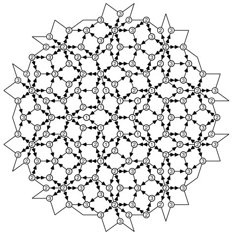
FIG. 3.: The double-arrow potential for a patch of the Penrose tiling.

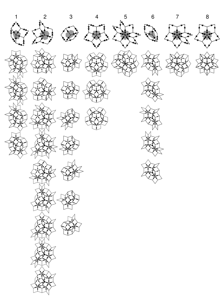
FIG. 4.: The eight vertex types of the Penrose tiling (top row) with the corresponding Voronoi cells (shaded), and the corresponding second-order vertex types (below).

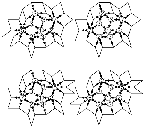
FIG. 5.: Second-order vertex types corresponding to a central vertex of type 1. Here, the encircled numbers denote the vertex types, not the potential.

FIG. 6.: Wave functions (21) for four different values $\beta=0.1$, $0.2$, $0.6$, and $0.9$. On a finite patch of ${\cal N}=16\,757$ vertices obtained by sevenfold inflation of a vertex of type $4$, the wave function has been normalized to $\sum_{i}|\phi_{i}|^{2}=1$. The radii of the circles encode $|\phi_{i}|^{2}$, in units of the edge length they have been chosen as $R=0$ for ${\cal N}|\phi|^{2}<10^{-2}$, $R=1.8\log(10^{2}{\cal N}|\phi|^{2})/\log(10^{4})$ for $10^{-2}\leq{\cal N}|\phi|^{2}\leq 10^{2}$ and $R=1.8$ for ${\cal N}|\phi|^{2}>10^{2}$.

FIG. 7.: Relation of the Voronoi cells of the Penrose tiling (thin lines) and their two-fold deflation (thick lines). The eight patches are obtained by a two-fold inflation of the eight vertex types (see Fig. 4). The numbers denote the change of the double-arrow potential with respect to the central Voronoi cell.

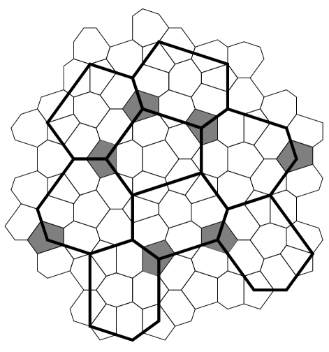
FIG. 8.: Voronoi cells of a patch of the Penrose tiling (thin lines) and of its two-fold deflation (thick lines). Shaded cells corresponding to vertex type 1 cannot be uniquely assigned to a cell of the deflated tiling.

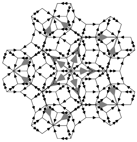
FIG. 9.: A vertex of type 8 (grey) together with its two-fold inflation (black).

FIG. 10.: The generalized dimensions $D_{q}$ for several values of $\beta$.

- [1] D. Shechtman, I. Blech, D. Gratias, and J.W. Cahn, Phys. Rev. Lett. 53, 1951 (1984).
- [2] T. Ishimasa, H.-U. Nissen, and Y. Fukano, Phys. Rev. Lett. 55, 511 (1985).
- [3] L. Bendersky, Phys. Rev. Lett. 55, 1461 (1985).
- [4] N. Wang, H. Chen, and K. H. Kuo, Phys. Rev. Lett. 59, 1010 (1987).
- [5] P. Bak, Phys. Rev. Lett. 56, 861 (1986).
- [6] R. Penrose, Bull. Inst. Math. Applications 10, 266 (1974); Eureka 39, 16 (1978), reprinted in: Math. Intell. 2, 32 (1979).
- [7] T.C. Choy, Phys. Rev. Lett. 55, 2915 (1985).
- [8] T. Odagaki and D. Nguyen, Phys. Rev. B 33, 2184 (1986).
- [9] M. Kohmoto and B. Sutherland, Phys. Rev. Lett. 56, 2740 (1986); Phys. Rev. B 34, 3849 (1986).
- [10] B. Sutherland, Phys. Rev. B 34, 3904 (1986).
- [11] T. Odagaki, Solid State Comm. 60, 693 (1986).
- [12] V. Kumar and G. Athithan, Phys. Rev. B 35, 906 (1987).
- [13] M. Kohmoto, Int. J. Mod. Phys. B 1, 31 (1987).
- [14] M. Arai, T. Tokihiro, T. Fujiwara, and M. Kohomoto, Phys. Rev. B 38, 1621 (1988).
- [15] Y. Liu and P. Ma, Phys. Rev. B 43, 1378 (1991).
- [16] J.Q. You, J.R. Yan, J.X. Zhong, and X.H. Yan, Europhys. Lett. 17, 231 (1992).
- [17] G.G. Naumis, R.A. Barrio, and C. Wang, Phys. Rev. B 50, 9834 (1994).
- [18] T. Rieth and M. Schreiber, Phys. Rev. B 55, 15827 (1995).
- [19] T. Rieth and M. Schreiber, J. Phys.: Condens. Matter 10, 783 (1998).
- [20] H. Tsunetsugu, T. Fujiwara, K. Ueda, and T. Tokihiro, J. Phys. Soc. Japan 55, 1420 (1986).
- [21] M. Arai, T. Tokihiro, and T. Fujiwara, J. Phys. Soc. Japan 56, 1642 (1987).
- [22] T. Fujiwara, M. Arai, T. Tokihiro, M. Kohomoto, Phys. Rev. B 37, 2797 (1988).
- [23] T. Tokihiro, T. Fujiwara, and M. Arai, Phys. Rev. B 38, 5981 (1988).
- [24] H. Tsunetsugu, T. Fujiwara, K. Ueda, and T. Tokohiro, Phys. Rev. B 43, 8879 (1991).
- [25] N.G. de Bruijn, Proc. Kon. Ned. Akad. Wet. A (Indagationes Mathematicae) 84, 39 and 53 (1981).
- [26] S. Wolfram, Mathematica: A System for Doing Mathematics by Computer (2nd edition), Addison–Wesley, Reading, Massachusetts (1991).
- [27] T.C. Halsey, M.H. Jensen, L.P. Kadanoff, I. Procaccia, and B.I. Shraiman, Phys. Rev. A 33, 1141 (1986).
- [28] M.V. Jarić, Phys. Rev. B 34, 4685 (1986).
- [29] M. Baake, P. Kramer, M. Schlottmann, and D. Zeidler, Int. J. Mod. Phys. B 4, 2217 (1990).