Magnetic properties of the three-band Hubbard model

Abstract

We present magnetic properties of the three-band Hubbard model in the para- and antiferromagnetic phase on a hypercubic lattice calculated with the Dynamical Mean-Field Theory (DMFT). To allow for solutions with broken spin-symmetry we extended the approach to lattices with AB-like structure. Above a critical sublattice magnetization $m_{d}\approx 0.5$ one can observe rich structures in the spectral-functions similar to the $t$-$J$ model which can be related to the well known bound states for one hole in the Neél-background. In addition to the one-particle properties we discuss the static spin-susceptiblity in the paramagnetic state at the points $\bf{q}=0$ and $\bf{q}=(\pi,\pi,\pi,\cdots)$ for different dopings $\delta$. The $\delta$-$T$-phase-diagram exhibits an enhanced stability of the antiferromagnetic state for electron-doped systems in comparison to hole-doped. This asymmetry in the phase diagram is in qualitative agreement with experiments for high-T_c materials.

1 Introduction and Model

One of the few undisputed facts about high-T_c materials is that all undoped high-$T_{c}$ compounds are insulators with antiferromagnetic ordering in the $\rm{CuO_{2}}$-planes at low enough temperatures Alm . Doping of the systems leads to a strong suppression of the antiferromagnetic order and eventually

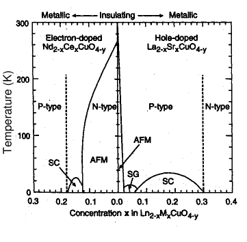
Figure 1: Experimental phase diagram for high-T_c compounds (taken from Alm ).

superconductivity sets in. While the explanation of this transition and the proximity of antiferromagnetism and superconductivity surely is the most fascinating aspect in the high-T_c compounds, there are a variety of other peculiarities that call for an explanation. One of these side aspects is the observation that, although the basic scenario is the same, hole and electron doped materials show an apparent qualitative difference in that the magnetic phase in the latter appears to be much more stable for the latter (cf. Fig. 1).

The physics in the insulating phase is well described by a Heisenberg model since charge fluctuations are suppressed by strong local correlations and, to a first approximation, one is left with the $\rm Cu$-spin degrees of freedom only. The exchange parameter of the resulting effective Heisenberg model is obtained from standard superexchange processes Anderson ; Zhang , induced by virtual hopping of a hole from one $\rm Cu$-ion to the neighbouring one over a nonmagnetic $\rm O$-ion.

At any finite doping one has to consider at least also the charge degrees of freedom on the copper sites and would then be left with the usual one-band Hubbard or $t$-$J$ model to describe the interplay between magnetic exchange and itinerancy. However, this scenario completely neglects the existence of the oxygen sites. That they are indeed important, at least for the magnetic properties, can be seen from the following qualitative argument: Due to the strong local correlations at the $\rm Cu$-sites, additional doped holes mainly occupy $\rm O$-sites. The spin of the hole at the $\rm O$-site induces an effective ferromagnetic interaction Aha between the neighbouring $\rm Cu$-spins, so that the antiferromagnetic ordering is strongly suppressed with increasing hole-doping. In the case of electron doping, on the other hand, the additional particle has to go to the copper sites due to Pauli’s principle, which effectively means that free spins are removed from the system. This obviously also leads to a suppression of magnetic order, but in a weaker fashion. Thus, in order to obtain a more realistic description of the physics of high-T_C compounds one has to take into account also the oxygen degrees of freedom and therefore one-band models like the standard Hubbard or $t$-$J$ model become inadequate.

The simpliest model which includes both the effect of strong correlations and the influence of the oxygen sites, is the three-band Hubbard model or Emery model Emer . The three-band Hubbard Hamiltonian reads

$$H = \sum\limits_{i,\sigma}\varepsilon_{d}d_{i\sigma}^{\dagger}d_{i\sigma}+\sum\limits_{j,\sigma}\varepsilon_{p}p_{j\sigma}^{\dagger}p_{j\sigma}$$ (1)

$$+ \sum\limits_{\langle ij\rangle,\sigma}t_{ij}\left(d_{i\sigma}^{\dagger}p_{j\sigma}+h.c.\right)+\sum\limits_{i}U_{d}\,n_{i\uparrow}^{d}n_{i\downarrow}^{d}\quad\mbox{,}$$

where the vacuum is defined as all orbitals in (1) filled with electrons. With this convention $d_{i\sigma}^{\dagger}(p_{j\sigma}^{\dagger})$ creates a hole in a $\rm{Cu}\,3d_{x^{2}-y^{2}}$-($\rm{O}\,2p_{x/y}$)-orbital at site $i(j)$ with spin $\sigma$ and $\varepsilon_{d}(\varepsilon_{p})$ are the corresponding on-site energies. $t_{ij}=\pm t$ denotes the nearest-neighbour hopping matrix-element between $\rm Cu$- and $\rm O$-sites and $U_{d}$ stands for the Coulomb-interaction of two holes, residing at the same $\rm Cu$-site $i$ with number operators $n_{i\sigma}^{d}$.

In this paper we want to study magnetic properties of the Hamiltonian (1) in the framework of the DMFT. In this theory the dynamical renormalizations of the one particle properties become purely local Metzner ; Mueller , so that they can be obtained from an effective impurity problem coupled to a self-consistent medium. Due to the additional orbital degreee of freedom in (1) the mapping on the corresponding effective impurity model is not unique. In order to treat local spin and charge fluctuations between the $\rm Cu$-site and the surrounding $\rm O$-sites better than on a mean-field level we use the approach, developed in ref. Schmalian , where a cluster of one $\rm{Cu}\,d$-orbital and a normalized bonding combination of the four surrounding $\rm O$-orbitals is coupled to the effective medium. This method indeed leads to the anticipated physics on the one-particle level, namely the formation of a low-lying singlet state – the Zhang-Rice singlet Zhang – and at half filling to a charge-transfer insulator Schmalian ; Zaanen ; Zoelfl in contrast to the Mott-Hubbard scenario for the one-band model. So far, however, only the paramagnetic state has been studied in ref. Schmalian . In ref. Doniach the metal-insulator (MI) transiton was studied with Quantum Monte Carlo in the context of the DMFT. There the model was also embedded on a bipartite lattice in order to take into account the antiferromagnetic symmetry breaking, but in this article the attention was called to the MI-transition.

In order to obtain the phase diagram or look at the behaviour in the antiferromagnetically ordered state the method has to be extended to allow for the calculation of susceptibilities or solve the DMFT equations for lattices with AB-like structure, respectively. A short review of this generalization together with the technique of calculating the magnetic susceptibility will be given in the next section, followed by the discussion of our results in section 3. The paper will conclude with a summary and outlook in section 4.

2 Method

2.1 The DMFT for the three-band model

Let us begin by summarizing the basic concepts introduced in Schmalian for the three-band Hubbard model. In order to construct the DMFT for a Cu-O plaquette, it is convenient to introduce the Fourier transform of the kinetic part of the Hamiltonian (1) after generalization to $d$ dimensions, which then reads Schmalian

$$H=\sum\limits_{{\bf k},\sigma}h_{\sigma}({\bf k})+\sum\limits_{i}U_{d}\,n_{i\uparrow}^{d}n_{i\downarrow}^{d}+H_{\rm non-bond}\quad\mbox{,}$$ (2)

with

$$h_{\sigma}({\bf k}) = \varepsilon_{d}d_{{\bf k}\sigma}^{\dagger}d_{{\bf k}\sigma}+\varepsilon_{p}p_{{\bf k}\sigma}^{\dagger}p_{{\bf k}\sigma}$$ (3)

$$+ \sqrt{2d}t\gamma_{\bf k}\left(d_{{\bf k}\sigma}^{\dagger}p_{{\bf k}\sigma}+h.c.\right)\quad\mbox{.}$$

Here, $d_{{\bf k}\sigma}$ is the Fourier transform of $d_{i\sigma}$ and $p_{{\bf k}\sigma}$ is the orthonormalized Fourier transform of the hybridizing combination of the oxygen orbitals surrounding a given copper site Zhang ; Schmalian . The $d-1$ linear combinations, which are orthogonal to $p_{{\bf k}\sigma}$ were collected into $H_{\rm non-bond}$ and will be dropped in the following, because they are decoupled from the remainder of the system. Finally, $\gamma_{\bf k}$ is given by $\gamma_{\bf k}^{2}=1-\frac{1}{d}\sum\limits_{\nu=1}^{d}\cos k_{\nu}$. In ref. Schmalian it was shown, that the rescaling

$$\sqrt{2d}t\gamma_{\bf k}\rightarrow 2t^{*}\gamma_{\bf k}^{*}$$ (4)

with $\gamma_{\bf k}^{*}=\sqrt{1-\frac{\varepsilon_{\bf k}}{\sqrt{2d}}}$, $t^{*}=\mbox{const.}\equiv 1$ and $\varepsilon_{\bf k}=\sum_{\nu=1}^{d}\cos k_{\nu}$ leads to a nontrivial limit for $d\rightarrow\infty$. The $d$-Green’s function in the DMFT now takes the form

$$G^{d}_{{\bf k}\sigma}(z)=\left[z-\varepsilon_{d}-\Sigma^{d}_{\sigma}(z)-\frac{4t^{*^{2}}-\frac{4t^{*^{2}}}{\sqrt{2d}}\varepsilon_{\bf k}}{z-\varepsilon_{p}}\right]^{-1}$$ (5)

The new ansatz by Schmalian et al. was to write the local $d$-Green’s function to be of the form Schmalian

$$G^{d}_{\sigma}(z)\begin{array}[t]{l}\displaystyle=\frac{1}{N}\sum\limits_{\bf k}G^{d}_{{\bf k}\sigma}(z)\\[14.22636pt] \displaystyle\stackrel{{\scriptstyle!}}{{=}}\Big{[}z-\varepsilon_{d}-\Sigma^{d}_{\sigma}(z)-\frac{4t^{*^{2}}}{z-\varepsilon_{p}-\Delta_{\sigma}(z)}\Big{]}^{-1}\;\;.\end{array}$$ (6)

In the DMFT the effective Cu-O cluster lives in a so-called effective medium, defined via

$${\cal G}_{\sigma}(z)^{-1}=G^{d}_{\sigma}(z)^{-1}+\Sigma^{d}_{\sigma}(z)=z-\varepsilon_{d}-\frac{4t^{*2}}{z-\varepsilon_{p}-\Delta_{\sigma}(z)}\;\;.$$ (7)

Note that in this form the coupling to the rest of the system, which is described by $\Delta_{\sigma}(z)$ happens through the $p$-states only. This representation of the local Green’s function is obviously not unique. One could also choose a representation for the local $d$-Green’s function of the form $G^{d}_{\sigma}(z)=\Big{[}z-\varepsilon_{d}-\Sigma^{d}_{\sigma}(z)-\Delta_{\sigma}(z)\Big{]}^{-1}$ where the resonance at $z=\varepsilon_{p}$ is included in $\Delta_{\sigma}(z)$. But from a numerical point of view the form (6) is more convenient because the singularity at $z=\varepsilon_{p}$ is not included in the hybridization function which therefore becomes smooth as a function of frequency. The form (6) of the local Green’s function is just the Dyson equation of an effective impurity problem consisting of one $d$- and one $p$-orbital, where only the $p$-orbital hybridizes with the conduction electrons (see eq. 13 in ref. Schmalian ).

2.2 DMFT for the Néel state

In the antiferromagnetic phase the period of the unit cell of the lattice is doubled due to the reduced translational symmetry. Consequently, the volume of the magnetic Brillouin zone (MBZ) is reduced to one-half of the volume in the paramagnetic state and the vector ${\bf Q}=(\pi,\pi,\pi,\cdots)$ becomes a reciprocal lattice vector. These changes in the symmetries of the system can be simply taken into account by introduction of an AB-sublattice structure Brand and reformulating the theory on an enlarged unit cell containing exactly one A- and one B-site. Since this procedure does not affect the local two-particle interaction in the Hamiltonian (2) we will concentrate on the kinetic part for the derivation of the resulting Hamilton matrix. We first split the kinetic part of (2) in the following way:

$$H={\sum\limits_{{\bf k}\in{\rm MBZ},\sigma}}\left\{h_{\sigma}({\bf k})+h_{\sigma}({\bf k+Q})\right\}$$ (8)

Note that the $\bf k$-sum runs over ${\bf k}$-points in the reduced Brillouin zone only! Rewriting (8) in terms of the linear combinations

$$\begin{array}[]{lcl}\displaystyle d_{A/B{\bf k}\sigma}&=&\frac{1}{\sqrt{2}}\left(d_{{\bf k}\sigma}\pm d_{{\bf k+Q}\sigma}\right)\\[14.22636pt] \displaystyle p_{A/B{\bf k}\sigma}&=&\frac{1}{\sqrt{2}}\left(p_{{\bf k}\sigma}\pm p_{{\bf k+Q}\sigma}\right)\quad\mbox{,}\end{array}$$ (9)

acting on the A- or B-sublattice, respectively, one obtains

$$H={\sum\limits_{{\bf k}\in{\rm MBZ},\sigma}}\Psi_{{\bf k}\sigma}^{\dagger}\underline{\underline{H}}_{\sigma}({\bf k})\Psi_{{\bf k}\sigma}\;\;.$$ (10)

For simplicity we introduced a spinor notation for the operators $\Psi_{{\bf k}\sigma}^{\dagger}=(d_{A{\bf k}\sigma}^{\dagger}\,p_{A{\bf k}\sigma}^{\dagger}\,d_{B{\bf k}\sigma}^{\dagger}\,p_{B{\bf k}\sigma}^{\dagger})$ and the Hamilton matrix on the sublattices

$${\underline{\underline{H}}}_{\sigma}({\bf k})=\left(\begin{array}[]{cccc}\varepsilon_{d}+\Sigma_{A}^{\sigma}&\Pi^{+}_{{\bf k}}&0&\Pi^{-}_{{\bf k}}\\ \Pi^{+}_{{\bf k}}&\varepsilon_{p}&\Pi^{-}_{{\bf k}}&0\\ 0&\Pi^{-}_{{\bf k}}&\varepsilon_{d}+\Sigma_{B}^{\sigma}&\Pi^{+}_{{\bf k}}\\ \Pi^{-}_{{\bf k}}&0&\Pi^{+}_{{\bf k}}&\varepsilon_{p}\end{array}\right)\quad\mbox{.}$$ (11)

The quantities $\Sigma_{A/B}^{\sigma}$ denote the local self-energies due to the two particle term in (2) on A/B-sublattice sites, which are different in the antiferromagnetic state. Furthermore $\Pi^{\pm}_{{\bf k}}=\frac{2t^{*}}{\sqrt{2}}\left(\gamma_{\bf k}^{*}\pm\gamma_{\bf k+Q}^{*}\right)$. For the $d$-components of the Green’s function matrix we finally obtain

$$\underline{\underline{G}}_{d}^{\sigma}({\bf k},z)=C_{{\bf k}\sigma}\left(\begin{array}[]{cc}\xi_{B}^{\sigma}&-\frac{\displaystyle 4t^{*^{2}}\varepsilon_{\bf k}}{\displaystyle\sqrt{2d}\xi_{p}}\\ -\frac{\displaystyle 4t^{*^{2}}\varepsilon_{\bf k}}{\displaystyle\sqrt{2d}\xi_{p}}&\xi_{A}^{\sigma}\end{array}\right)$$ (12)

with $C_{{\bf k}\sigma}=\left[\xi_{A}^{\sigma}\xi_{B}^{\sigma}-\left(\frac{4t^{*^{2}}\varepsilon_{\bf k}}{\sqrt{2d}\xi_{p}}\right)^{2}\right]^{-1}$, $\xi_{p}=z+\mu-\varepsilon_{p}$ and $\xi_{A/B}^{\sigma}=z+\mu-\varepsilon_{d}-\Sigma_{A/B}^{\sigma}-\frac{4t^{*^{2}}}{\xi_{p}}$. The local Green’s function is obtained by taking one of the diagonal elements and summing over $\bf k$ with the result

$$G_{d,A/B}^{\sigma}(z)=\int\limits_{-\infty}^{\infty}d\varepsilon\,\rho_{o}(\varepsilon)\frac{\xi^{\sigma}_{B/A}}{\xi_{A}^{\sigma}\xi_{B}^{\sigma}-\left(\frac{{\displaystyle 4t^{*^{2}}\varepsilon}}{{\displaystyle\xi_{p}}}\right)^{2}}\quad\mbox{,}$$ (13)

where the density of states $\rho_{o}(\varepsilon)$ corresponding to the dispersion $\varepsilon_{\bf k}$ was introduced. In the paramagnetic state, where $\xi^{\sigma}_{A}=\xi^{\sigma}_{B}$, one immediately recovers the result of section 2.1.

In the antiferromagnetic state it is sufficient to perform the calculations for the A-sublattice only due to the additional symmetry Brand $G_{d,A}^{\sigma}=G_{d,B}^{\bar{\sigma}}$ and use the spin-index for book-keeping. The actual calculation is now a straightforward extension of the method used in ref. Schmalian for the paramagnetic phase. The local nature of the selfenergies allows the mapping of the lattice problem on an effective impurity-problem, consisting of a $d$-orbital and the orthonormalized hybridizing combination of the four surrounding $p$-orbitals, coupled to the effective medium, which is described by the propagator (7) and has to be determined selfconsistently. Again, the coupling to the surrounding clusters is assumed to happen through the $p$-states only.

The remaining local problem is solved with the resolvent method Kei ; Bickers and an extended version of the so called Non Crossing Approximation (NCA) Bickers , where the 16 local eigenstates of the impurity are coupled through the hybridization-function $\Delta^{\sigma}(z)$ Schmalian .

2.3 On the calculation of the magnetic susceptibility

On the one-particle level one can obtain magnetic properties by applying a staggered magnetic field and calculating the sublattice magnetization. This technique is very tedious so that we used another method for calculating the magnetic phase diagram.

In addition to the one-particle properties the DMFT also allows to calculate two-particle correlation functions, e.g. the magnetic susceptibility consistently. In analogy to the one-particle case the two-particle self energy becomes purely local in the limit $d\rightarrow\infty$ Brand ; Jarr . This enables us to extract the two-particle self-energy from the effective local problem Jarr ; MJ ; ThP and use it to determine the two-particle correlation function for the lattice. Since the local two-particle propagator is a function of three frequencies in the most general case the algorithm works best for Matsubara frequencies, because all quantities can be represented as matrices in this case. For details of the method see e.g. ref. ThP .

The choice of the cluster as effective impurity and the finite value of $U_{d}$ results in 16 local eigenstates. This leads to a huge number of diagrams for the local two-particle propagator, which have to be calculated as functions of three frequencies and summed up numerically. Although the problem of generating the correct diagrams for the local two-particle propagator can be automated and handled by the computer, the remaining numerical task is still formidable and restrict our calculations to the evaluation of the static susceptibility for the time being. Nevertheless, the study of the dynamical susceptibility is in principle also possible ThPII and will be the subject of a forthcoming publication.

3 Results

3.1 Susceptibility and phase diagram

Let us start the discussion of our results with the magnetic susceptibility. We calculated the static magnetic susceptibility of the $\rm Cu$-spins in the paramagnetic phase at the points ${\bf q}=0$ and ${\bf q}={\bf Q}$, which give the homogeneous and staggered susceptibilities, respectively. For the parameters of the three-band Hubbard model we have chosen $U_{d}=2\Delta=7t^{*}$, where the charge transfer gap $\Delta$ is defined by $\Delta=\varepsilon_{p}-\varepsilon_{d}$. Fig. 2a shows typical results for these two susceptibilities as a function of temperature T for a hole-doping $\delta=n_{d}+n_{p}-1=0.1$.

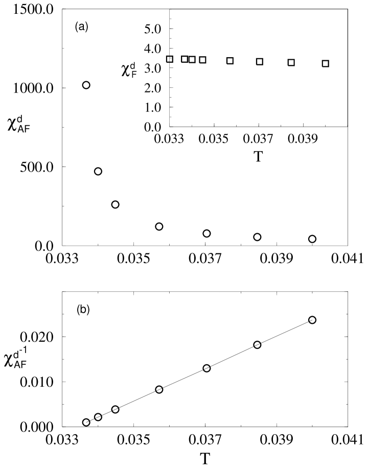
Figure 2: Homogeneous ($\chi^{d}_{F}$) and staggered ($\chi^{d}_{AF}$) susceptibilities (a) and inverse staggered susceptibility (b) for 10% hole-doping and parameters as given in the text.

For the above choice of $U_{d}$ and $\Delta$ we observe a finite and slowly varying ferromagnetic susceptibility $\chi_{F}^{d}(T,\delta)$, which does not show any tendency towards an instability in the calculated region of temperatures and dopings. The antiferromagnetic susceptibility $\chi_{AF}^{d}(T,\delta)$, on the other hand, varies strongly as a function of temperature and diverges at a finite temperature $T=T_{N}$. Fig. 2b shows the inverse staggered susceptibility for the same parameters. As expected we find the linear variation of $\chi_{AF}^{-1}$, which is typical for a mean-field theory. By calculating the inverse susceptibility for different dopings $\delta$ we obtain the $\delta$-$T$-phase-diagram, shown in Fig. 3.

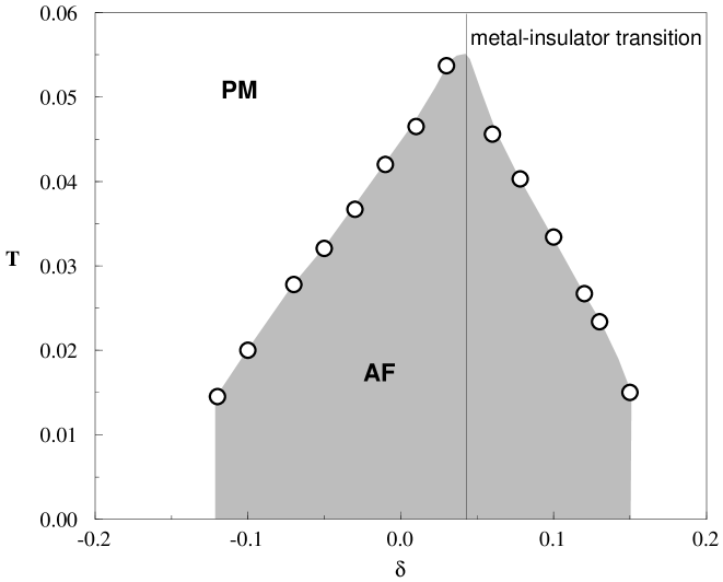
Figure 3: Magnetic phase-diagram for the 3-band Hubbard model on a hypercubic lattice for $U_{d}=2\Delta=7t^{*}$.

Note, that half-filling ($\delta=0$) does not coincide with the MI-transition. This is so because for the used parameter values of $U_{d}$ and $\Delta$ the metal-insulator-transition is shifted towards larger hole-filling values $n>1$. Obviously the highest value for the Neél temperature is achieved at the metal-insulator-transition and not at half-filling. As already observed for the one band model MJ ; ThP the antiferromagnetic phase is strongly suppressed upon doping. However, in contrast to the former case one recognizes a pronounced asymmetry in the Neél temperature with respect to hole- and electron-doping. This stronger sensistivity of the antiferromagnetic ordered state in the case of hole doping compared to electron doping is qualitatively in good agreement with experiments (see Fig. 1) and is a direct consequence of the oxygen degrees of freedom. The present large $D$ treatment however neglects short range order phenomena so that the argumentation of ref. Aha concerning the frustration of the AF-order by hole doping does not hold on this level. But nevertheless the oxygen degrees of freedom cause a particle hole asymmetry in the half filled three band model which yields the calculated asymmetry in the phase diagram in this large $D$ approach.

In our calculations the ordered phase is stable up to $\delta\approx 0.18$ for low enough temperatures (cf. Fig. 3). Experiments and other theoretical calculations show much stronger suppression of the antiferromagnetic ordering with doping Alm . The tendency to overestimate the magnetic phase boundary is typical for mean field theories, since they completely neglect fluctuations, which strongly renormalize transition temperatures.

3.2 Spectral functions in the ordered phase

With the generalized equation (13) it is also possible to perform calculations in the antiferromagnetic phase. To allow for solutions with finite sublattice magnetization$m_{d}=\left|\left\langle n_{d\uparrow}^{A/B}-n_{d\downarrow}^{A/B}\right\rangle\right|$ we apply a small symmetry-breaking staggered magnetic field $h({\bf r}_{i})=he^{i{\bf Q}\cdot{\bf r}_{i}}$ in $z$-direction at the beginning of our iteration procedure, which is turned off after a few iterations.

In the following we concentrate on the $d$-part of the spectrum $A_{d}^{\sigma}(\omega)=-\frac{1}{\pi}{\rm Im}G_{d,A}^{\sigma}(\omega+i\delta)$ on the A-sublattice, since the $p$-part shows exactly the same features as the $d$-part, only with different spectral weights for the various bands. Fig. 4a,b,c shows the typical behaviour as the temperature $T$ is lowered for fixed values of the parameters $U_{d}=2\Delta=7t^{*}$ at finite doping $\delta=0.015$.

Figure 4: $d$-spectral function for the majority (full curves) and minority spin (dashed curves) for $U_{d}=2\Delta=7t^{*}$, fixed doping $\delta=0.015$ (below the MI-transition (cf. Fig.3)) for various temperatures $\beta=18/t^{*}$ (a), $\beta=20/t^{*}$ (b) and $\beta=22/t^{*}$ (c) and for $\delta=0.063$ (above the MI-transition) and $\beta=22/t^{*}$ (d)

For $\beta=18/t^{*}$ the system is in the paramagnetic state (cf. Fig. 4a), where the general equation (13) reduces to the form (6). We find the same result for the $d$-part of the spectrum as in ref. Schmalian , where a detailed discussion of the various bands concerning their doping dependence, transfer of spectral weight and the evolution of coherent quasiparticles near the Fermi-energy can be found. Let us just briefly mention the important low energy parts, namely the so-called lower Hubbard band at $\omega<0$ in the spectrum of Fig. 4, which has mainly $d$-character, and the Zhang-Rice band right above the gap, which is generated by the singlet combination of the $p$-and $d$-states on one plaquette Schmalian . Note that $\delta>0$ although the chemical potential is located in the lower Hubbard band. Therefore the MI-transition occurs at larger filling values as already mentioned in section 3.1. With decreasing temperature the system enters the antiferromagnetic phase and the spectral functions of up and down spin become inequivalent (cf. Fig. 4b), yielding a finite sublattice magnetization $m_{d}$. Note that the major effect is a transfer of spectral weight from the minority spin to the majority spin. In addition the peaks in the spectra are slightly shifted in energy with respect to each other. This effect can be ascribed to an internal molecular field, generated by the finite sublattice magnetization. Therefore, measuring the energy shift one can calculate the internal molecular field and from this the exchange parameter $J$ of a corresponding tJ-model. For still lower temperatures the sublattice magnetization increases and above a value of $m_{d}\approx 0.5$ a pronounced multipeak structure is evolving (see Fig. 4c). Fig. 4d shows the spectral function for the same system parameters and sublattice magnetization as in Fig. 4c but with the chemical potential right above the gap. Also in this regime the same multipeak structure occurs and the spectral function shows little difference to Fig. 4c. Only the peaks next to the chemical potential have more spectral weight compared with Fig. 4c.

These regular resonances were previously found in DMFT calculations of the tJ-model Obermeier . There the multiple peaks could be related to bound states of one single hole in the Neél background. In ref. Strack it was shown, that this special problem can be solved exactly for $d=\infty$ and $T=0$ within the tJ-model. The most important physical aspect is, that the moving hole feels a binding potential proportional to $J$, growing linearly with the distance from its starting point due to the breaking of antiferromagnetic bonds during its motion Strack ; Obermeier . This linear potential leads to a sequence of discrete poles at frequencies Strack

$$\omega_{n}=-2\hat{t}-\frac{J^{*}}{2}-a_{n}\hat{t}\left(\frac{J^{*}}{2\hat{t}}\right)^{\frac{2}{3}}$$ (14)

as spectrum for the one particle excitations. Here, the $a_{n}$ denote the zeros of the Airy function $Ai\left(4\hat{t}/J^{*}\right)$, and the renormalized parameters $\hat{t}$ and $J^{*}$ are given by $\hat{t}=t\sqrt{2d}$, $J^{*}=J2d$. These exact results can be compared directly to the resonances, found in the DMFT calculations for the tJ-model Obermeier . Since the model used in our calculations is fundamentally different from the tJ-model and also from the one-band Hubbard model, the relevance of this physically intuitive picture to it and especially the proper choice of the parameters for an effective tJ-model to describe the low energy properties is not clear a priori. The approach chosen here is to fix the hopping to $t^{2}/\Delta$, which reproduces the free bandwidth. In our case we determine an effective exchange interaction $J^{*}$ from the energy shift $\Delta E=J^{*}m_{d}$ of the bands. Note that this is just the energy shift of the spin-up and spin-down bands of a corresponding tJ-model, treated on a mean-field level Mueller ; Obermeier ; Itz . Another possibilty to obtain the exchange integral $J$ is to use the result of a Schrieffer-Wolf transformation of the 3-band Hubbard model, see e.g. Zaanen . However this transformation holds only for large values of $U_{d}$ and $\Delta$, so that we do not expect this procedure to give a meaningful result for our parameter values.

Fixing the paramters in eq. (14) as discussed above, we can indeed directly compare our results with the discrete spectrum (14). Fig. 5 shows some examples for the fit of the low energy part of the $d$-spectrum $A_{d}^{\sigma}(\omega)$ by the discrete spectrum (14) at fixed doping $\delta=0.015$ and sublattice magnetization $m_{d}=0.60$ for various parameters $U_{d}=2\Delta$.

Figure 5: Comparison of the low energy part of the $d$-spectrum with the exact results (vertical lines), given by equation (14).

Note, that the energy scales of up- and down-spin in Fig. 5 are already shifted by $\pm\Delta E/2$ respectively, so that the resonances of majority- and minority-spin bands coincide. We find quite good agreement with the distance of the peak positions. The broadening is expected to result from finite temperature, sublattice magnetization and doping effects Obermeier . This means that the tJ-model with proper choice of the parameters $t$ and $J$ seems to reproduce the low energy one-particle dynamics of the three-band Hubbard model in $d=\infty$ correctly, even in the antiferromagnetic state. In addition, the basic physical picture for the multipeak structures observed for low temperatures appears to be the same as in the simple one-band models.

In order to gain more insight in the effect of doping on these multipeak structure we investigated the spectrum at larger doping far away from the MI-transition. Fig. 6 shows the results for the $d$-part of the spectrum for the same system parameters and sublattice magnetization as in Fig. 4c,d at $\beta=50/t^{*}$ but at larger doping $\delta=-0.08$ (a) and $\delta=0.13$ (b).

Figure 6: $d$-spectral function for the majority (full curves) and minority spin (dashed curves) for $U_{d}=2\Delta=7t^{*}$ and $\beta=50/t^{*}$ at $\delta=-0.08$ (a) and $\delta=0.13$ (b).

In the electron (Fig. 6a) as well as in the hole doped regime (Fig 6b) only the resonances next to the chemical potential survive. Due to the larger doping there are more electrons/holes in the system whose paths can intersect and restore the antiferromagnetic background. Therefore the electrons/holes become more mobile and the resonances at higher energies are washed out.

In finite dimensions the string picture for one hole in the antiferromagnetic background no longer holds and is correct only up to order $\frac{1}{d^{2}}$ Strack due to the possibility of paths which intersect and touch themselves Trug . Second, fluctuations become more important which can restore the antiferromagnetic background. Thus in low dimensions we expect that the multipeak structure at finite doping will dissappear.

4 Summary

In this paper we presented results for the magnetic properties of the three-band Hubbard model in the limit of high spacial dimensions. These were obtained in the framework of the Dynamical Mean Field Theory, which enabled us to calculate the one particle spectrum as well as two particle correlation functions, namely the magnetic susceptibility. From this we evaluated the $\delta$-$T$-phase diagram, which shows strong suppression of the antiferromagnetic state upon doping. In contrast to one-band models the ordered state is found to be more sensitive upon doping in the case of hole doping in comparison to electron doping. This asymmetric behaviour is qualitatively in good agreement with experiments. The spectral function for single particle excitations in the antiferromagnetic phase shows pronounced features above a sublattice magnetization $m_{d}\approx 0.5$. These structures are similar to those found in the tJ-model for the special case of one single hole, moving in the Neél background and can be understood by the binding of one hole in a string potential. A quantitive fit of the spectral functions by the exact results for the special case for the tJ-model shows quite good agreement, so that the tJ-model seems to reproduce the correct physics of the three-band Hubbard model as long as one is only interrested in the low energy one-particle physics.

In low dimensions fluctuations become more important which will destroy the multiple peaks found in the spectral function for $d=\infty$. Thus these peaks have not yet been observed in experiments.

References

- (1) C. Almasan, M. B. Maple, Chemistry of High-Temperature Superconductors, edited by C. M. Rao, World Scientific, Singapore (1991)
- (2) P. W. Anderson, Phys. Rev. 124, 41 (1961)
- (3) F. C. Zhang, T.M. Rice, Phys. Rev. B 37, 3759 (1988)
- (4) A. Aharony et al., Phys. Rev. Lett. 60, 1330 (1988); R. J. Birgeneau, M. A. Kastner, A. Aharony, Z. Phys. B 71, 57 (1988)
- (5) V. J. Emery, Phys. Rev. Lett. 58, 2794 (1987)
- (6) W. Metzner, D. Vollhardt, Phys. Rev. Lett. 62, 324 ( 1989)
- (7) E. Müller-Hartmann, Z. Phys., B 74, 507 (1989)
- (8) J. Schmalian, P. Lombardo, M. Avignon, K. H. Bennemann, Physica B 222-224, 602 (1996); P. Lombardo, M. Avignon, J. Schmalian, K. H. Bennemann, Phys. Rev. B 54, 5317 (1996)
- (9) J. Zaánen, A. M. Oleś, Phys. Rev. B 37, 9423 (1988)
- (10) M. B. Zoelfl, Th. Maier, Th. Pruschke, J. Keller, to be published
- (11) H. Watanabe, S. Doniach, Phys. Rev. B 57, 3829 (1998)
- (12) U. Brandt, C. Mielsch, Z. Phys., B 79, 295 (1990)
- (13) H. Keiter, J. C. Kimball, Phys. Rev. Lett. 25, 672 (1970)
- (14) N. E. Bickers, D. L. Cox, J. W. Wilkins, Phys. Rev. B 36, 2036 (1987)
- (15) Th. Pruschke, D. L. Cox, M. Jarrell, Phys. Rev. B 47, 3553 (1993)
- (16) M. Jarrell, Th. Pruschke, Z. Phys. B 90, 187 (1993)
- (17) Th. Pruschke, Q. Qin, Th. Obermeier, J. Keller, J. Phys. Condens. Matter 8, 3161, (1996)
- (18) Th. Pruschke, Th. Obermeier, J. Keller, Physica B 230-232, 895(1997).
- (19) Th. Obermeier, Th. Pruschke, J. Keller, Ann. Physik 5, 137 (1996)
- (20) R. Strack, D. Vollhardt, Phys. Rev. B 46, 13852 (1992)
- (21) C. Itzykson, J.M. Drouffe, Statistical Field Theory Vol. I & II, Cambridge University Press, Cambridge (1989)
- (22) S. A. Trugman, Phys. Rev. B 41 892 (1990)