Free vortex and vortex-pair lifetimes in classical two-dimensional easy-plane magnets

Abstract

We report numerical simulation results for free-vortex lifetimes in the critical region of classical two-dimensional easy-plane ferro- and antiferromagnets having three-component order parameters. The fluctuations in the vortex number density in a spin dynamics simulation were used to estimate the lifetimes. The observed lifetimes are of the same order of magnitude but smaller than the characteristic time-scale above which a phenomenological ideal vortex-gas theory that has been used to account for the central peak in the dynamic structure factor $S^{\alpha\alpha}({\bf q},\omega)$ is expected to be valid. For strong anisotropy, where the vortices are in-plane, the free vortex lifetimes for ferromagnets and antiferromagnets are the same, while for weak anisotropy, where the vortices have nonzero out-of-easy-plane components, the lifetimes in antiferromagnets are smaller than in ferromagnets. The dependence of the free-vortex and total vortex densities on the size dependent correlation length in the critical region is examined. We also determined the lifetimes of vortex-antivortex pairs for $T=T_{\mbox{KT}}$ and well below $T_{\mbox{KT}}$. The observed time-scales are very short, and the observed pair densities are extremely small. These results suggest that pair creation and annihilation are unlikely to play any role in the central peak in $S^{xx}({\bf q},\omega)$ observed in computer simulations for the ferromagnetic model for $T\leq T_{\mbox{KT}}$.

I Introduction

The interpretation of the central peak in the dynamic structure factor $S^{\alpha\alpha}({\bf q},\omega)$ in easy-plane layered ferromagnets (FM) and antiferromagnets (AFM) is currently based on the phenomenological theory developed by Mertens et al.[1, 2, 3, 4, 5, 6, 7] The central peak is observed for $T>T_{\mbox{KT}}$ ($T_{\mbox{KT}}$ is the Kosterlitz-Thouless transition temperature) and the theory accounts for it within the frame of a dilute gas of free vortices effectively assuming infinite free-vortex lifetime. It is of importance to determine the free-vortex lifetime to find out the interval of applicability of the theory as well as to understand the time scale of the processes which account for the finite lifetime. We have developed a method to calculate the vortex lifetime and we present here our results obtained from combined cluster Monte Carlo (MC) and spin dynamics simulations. We believe that these are the first reported free-vortex lifetimes in AFM for the system Hamiltonian we have considered.

The intensity and width of the central peak predicted by the dilute-vortex-gas theory depend on the free vortex density $N_{v}$ and the rms vortex velocity $\bar{u}$. A free vortex is assumed to exist longer than a characteristic observation time

$$1/\gamma=2\xi/\sqrt{\pi}\bar{u},$$ (1)

where $\xi$ is the correlation length. It is assumed that the vortices have a Maxwellian velocity distribution. If this theory is valid, it could, in principle, allow one to determine the average free vortex velocity $\bar{u}$ and the correlation length $\xi$ at a given temperature by experimentally measuring the shape of the central peak, knowing the strength of the Heisenberg exchange interaction for the magnetic material.

The FM and AFM static properties on a square lattice (or other bi-partite lattice) are identical (the spins on one of the sublattices in the AFM are inverted when compared with the spins in the FM) while their dynamic properties differ.[8] In particular, the out-of-plane tilting of spins near the core of a vortex produces a nonzero topological charge (or gyrovector[9, 10]) for vortices in the FM model. The gyrovector plays an important role in determining how the motion of an individual vortex is influenced by effective fields due to neighboring vortices, and it appears together with an effective mass in a collective coordinate equation that describes the motion of a vortex center.[11] However, the gyrovector is always zero for vortices in the AFM model, and, the effective mass for vortices in the AFM model is much smaller than for vortices in the FM model.[12] For these reasons we expect that the FM and AFM models could have quite different vortex lifetimes, and therefore contrast the lifetimes measured for the AFM model with those we have determined previously for the FM model.[13]

II The Model

The Hamiltonian of the model is

$$H=-J\sum_{\langle i,j\rangle}(S_{i}^{x}S_{j}^{x}+S_{i}^{y}S_{j}^{y}+\lambda S_{i}^{z}S_{j}^{z}),$$ (2)

where the classical spins $\mbox{\bf S}_{i}=(S^{x}_{i},\ S^{y}_{i},\ S^{z}_{i})$ are vectors on the unit sphere $S^{2}$, the sum is over nearest-neighbor sites of a square lattice, the easy-plane anisotropy parameter $\lambda$ varies in the interval $0\leq\lambda<1$, and $J>0$ for FM and $J<0$ for AFM. We assume that $J$ has energy units, time is measured in units of $\hbar/J$ and temperature in $J/k_{B}$; the spins are dimensionless.

The static critical behavior of this model is well-described by the extensively studied classical XY model (the two-dimensional $O(2)$ model) but because of the possibility for spin fluctuations in one more degree of freedom (the out-of-plane $S^{z}$ fluctuations) the properties of the XY model will be observed at lower temperatures here.

Long-range order cannot exist for any nonzero temperature in these models,[14] but Berezinskii[15] showed the existence of a phase transition which was understood by Kosterlitz and Thouless[16] to occur through unbinding of pairs of nonlinear topological excitations–vortices. The critical properties of the XY model[17] as well as the low-temperature phase are of considerable interest to the physics of low-dimensional magnetism because there are a number of materials which are effectively considered as two-dimensional magnetic systems[18] and the Hamiltonian (2) is the simplest model to study their properties. These are layered crystals with intralayer exchange interaction much greater than their interlayer exchange (more than two or three orders of magnitude greater) and there are observed both ferromagnets[19, 20, 21, 22] (e.g. K₂CuF₄, (CH₃NH₃)₂CuCl₄, (C₂H₅NH₃)₂CuCl₄, Rb₂CrCl₄) and antiferromagnets[23, 24, 25] (like BaNi₂(PO₄)₂, BaCo₂(AsO₄)₂). The intralayer exchange interaction is more than $10^{-3}$ orders of magnitude smaller than the intralayer exchange in the graphite-intercalated CoCl₂ which has been studied in detail by Wiesler et al.[26] There are magnetic lipid monolayers,[27] e.g. the compound Mn(C${}_{1}8$H${}_{3}5$O₂)₂, which are true two-dimensional magnets.

When the anisotropy parameter $\lambda$ is less than a critical value, $\lambda_{c}$ which is lattice dependent,[28] only in-plane static vortex spin configurations ($\left<S^{z}\right>=0$) are stable, while for $\lambda>\lambda_{c}$ only static vortices with nonzero out-of-plane ($\left<S^{z}\right>\neq 0$) spin components are stable. The critical anisotropy parameter $\lambda_{c}$ has recently been determined[29] with good precision and for the square lattice $\lambda_{c}\approx 0.7034$.

III Dynamics

The differences in dynamical properties of FM vs. AFM not only appear in the vortex properties, but also in the spinwave-vortex interaction and the spinwaves alone. The spin-wave excitations have a single branch for FM while there are two branches for AFM due to the two different spin sublattices. The spin waves are either in-plane or out-of-plane depending on the value of $\lambda$. Ivanov et al.[30] found a localized mode for the out-of-plane vortex in AFM which appears in the gap between the two spin-wave branches. Wysin et al.[31] have also shown that even for the in-plane vortices in the AFM model, this localized mode is still present. For the FM model, in contrast, only quasi-local spinwave modes appear on a vortex (where the $S^{z}$ component of the mode is localized near the vortex core while the $S^{x},S^{y}$ components of the mode are extended).

In the ideal vortex-gas theory,[1, 2, 3, 4, 5, 6, 7] the motion of free vortices in a temperature interval just above $T_{\mbox{KT}}$ is assumed ballistic and leads to central peaks in both in-plane $S^{xx}(q,\omega)$ ($S^{xx}=S^{yy}$ due to the symmetry of the Hamiltonian) and out-of-plane $S^{zz}(q,\omega)$ dynamic structure factors, where $S^{\alpha\alpha}(q,\omega)$ ($\alpha=x,y,z$) is the space-time Fourier transformation of the correlation function $\langle S^{\alpha}(\mbox{\bf r},t)S^{\alpha}(\mbox{\bf 0},0)\rangle$. The central peak (CP) of the in-plane dynamic structure factor is predicted to have a squared Lorentzian shape

$$S^{xx}(\mbox{\bf q},\omega)={S^{2}\gamma^{3}\xi^{2}\over 2\pi\left[\omega^{2}+\gamma^{2}(1+(\xi q^{*})^{2})\right]^{2}},$$ (3)

where $\gamma$ is defined in (1). The CP is located at $\mbox{\bf q}^{*}=(0,0)$ for FM ($\mbox{\bf q}^{*}\equiv\mbox{\bf q}$) and at the Bragg point $\mbox{\bf K}=(\pi,\pi)$ for AFM ($\mbox{\bf q}^{*}\equiv\mbox{\bf K}-\mbox{\bf q}$). A weaker CP is predicted for the out-of-plane dynamic structure factor for any $\lambda$, due to correlations caused by vortex motion. It is located at $\mbox{\bf q}=(0,0)$ for both FM and AFM. Its intensity is proportional to the free vortex density $N_{v}$ and has Gaussian shape

$$S^{zz}(q,\omega)={N_{v}\bar{u}\over 32f^{2}_{\lambda}J^{2}\sqrt{\pi}q}\exp\left(-\left(\omega/\bar{u}q\right)^{2}\right),$$ (4)

where $f_{\lambda}=1-\lambda$ for FM and $1+\lambda$ for AFM. For $\lambda>\lambda_{c}$, the out-of-plane vortex spin asymptotic behavior is known $S^{z}(r)\sim\sqrt{r_{v}/r}\exp(-r/r_{v})$, where $r_{v}=\sqrt{\lambda/(1-\lambda)}/2$ is considered as the vortex core radius and $r$ is the distance from the vortex center. This asymptotic form is used to calculate $S^{zz}(q,\omega)$ for both FM[2] and AFM[6, 7] leading to an additional CP only for $\lambda>\lambda_{c}$ with Gaussian shape

$$S^{zz}(q^{*},\omega)\sim{N_{v}\bar{u}\over{q^{*}}^{3}}\exp\left(-\left(\omega/\bar{u}q^{*}\right)^{2}\right),$$ (5)

and again $\mbox{\bf q}^{*}\equiv\mbox{\bf q}$ for FM and $\mbox{\bf q}^{*}\equiv\mbox{\bf K}-\mbox{\bf q}$ for AFM. By measuring the width and the integrated intensity of the CP one can determine $\bar{u}$ and $\xi$ and compare with independent theoretical results. We compare the characteristic times $1/\gamma$ obtained in this way with our results on the vortex lifetime.

Thus, we expect that vortices in FM and AFM for $\lambda<\lambda_{c}$ have quite similar dynamics (and similar lifetimes), which is reflected particularly in their similar in-plane correlations. However, the nonzero gyrovector for FM vortices is present for $\lambda>\lambda_{c}$. This is an additional term in the vortex equation of motion for the FM case, which is absent for AFMs. Furthermore, the effective vortex mass of AFM vortices has been estimated to be smaller than for FM vortices[12] only for $\lambda>\lambda_{c}$. Because of these differences, we calculate the vortex lifetime for both $\lambda<\lambda_{c}$ and for $\lambda>\lambda_{c}$, with the expectation that larger differences should occur in the latter case.

In recent numerical simulations,[32] CP has been observed in $S^{xx}(q,\omega)$ for $T\leq T_{\mbox{KT}}$ and $\lambda=0$. It is not clear currently what causes the CP for $T\leq T_{\mbox{KT}}$. For these temperatures, the dominant excitations are spin waves and the vortices are bound in pairs with opposite vorticities. The vortex pairs should only renormalize the shape of the spin-wave peaks and should not lead to additional peaks as do the free vortices above $T_{\mbox{KT}}$. Nevertheless, we have calculated and checked the lifetime of vortex pairs below $T_{\mbox{KT}}$. We found that the observed pair lifetime is a very short time scale to be the relevant effect for the observed CP at these temperatures.

IV The Simulation

We simulate a system of classical spins (three-component unit vectors) on a square lattice with periodic boundary conditions and $L\times L$ number of sites, for sizes $L\leq 256$. First, we run Monte Carlo (MC) simulations to obtain initial equilibrium configurations (IC) and to calculate the correlation length and vortex densities. The obtained IC’s are then evolved in time using a fourth order Runge-Kutta method[33] to solve the Landau-Lifshitz equations of motion

$${d\mbox{\bf S}_{i}\over dt}=\mbox{\bf S}_{i}\times(-{\delta H\over\delta\mbox{\bf S}_{i}}),$$ (6)

where

$$-{\delta H\over\delta\mbox{\bf S}_{i}}=J\sum_{\langle j(i)\rangle}(S_{j}^{x}\mbox{\bf\^{x}}+S_{j}^{y}\mbox{\bf\^{y}}+\lambda S_{j}^{z}\mbox{\bf\^{z}}),$$ (7)

x̂, ŷ, and ẑ are unit vectors along the coordinate system axes. The sum is over the nearest neighbor sites of the site $i$.

We used a combination of Wolff’s one cluster algorithm[34] (for updating of the in-plane spin components $S_{i}^{x}$ and $S_{i}^{y}$), Metropolis’ algorithm,[35] and the over-relaxed algorithm[36] to update the spins in the MC part of the simulations. Each Monte Carlo step (MCS) through the system consists of three single-cluster updates, three Metropolis sweeps, and three over-relaxed sweeps. The use of Wolff’s algorithm is essential for reducing critical slowing down. The over-relaxed move on a classical spin consists of rotating the spin around the direction of the local field due to its nearest neighbor spins (assuming no external magnetic field) at an angle of $\pi$, i.e. if $\mbox{\bf\^{h}}=\mbox{\bf h}_{loc}/|\mbox{\bf h}_{loc}|$, then

$$\mbox{\bf s}_{new}=2(\mbox{\bf\^{h}}\cdot\mbox{\bf s}_{old})\mbox{\bf\^{h}}-\mbox{\bf s}_{old}.$$ (8)

The move is microcanonical and it also reduces critical slowing down even though it is a local move. The Metropolis algorithm is needed to satisfy ergodicity of the MCS for the Hamiltonian we study. The first 1000 to 5000 MCS were used for equilibration of the system and IC were written after each bin consisting of 2000 to 10000 MCS. Between 25 to 100 IC were produced for the spin dynamics simulations. The calculation of the correlation length and vortex density is from averages over 20 or 25 bins with measurements after each MCS and all estimated statistical errors are equal to the standard deviation of the bin averages.

The correlation length is determined by measuring[37, 38, 39]

$$\xi_{L}={1\over q}\sqrt{G(\mbox{\bf 0})/G(\mbox{\bf q})-1},$$ (9)

$$G(\mbox{\bf q})={1\over L^{2}}\left<\left|\sum_{\mbox{\bf r}_{i}}\exp(i\mbox{\bf q}\cdot\mbox{\bf r}_{i})\mbox{\bf S}_{i}^{\perp}\right|^{2}\right>,$$ (10)

where $\mbox{\bf S}_{i}^{\perp}=(S_{i}^{x},\,S_{i}^{y})$ is the in-plane spin vector. The wave-vector $\mbox{\bf q}=(2\pi/L,\ 0)$ is used, and $\mbox{\bf r}_{i}$ is the radius-vector of the $i$th lattice site. The correlation length $\xi_{L}$ obtained from Eq. (9) approaches the exact value as $O(q^{4})$ approaches zero when increasing the linear size of the system L.[38, 40] The finite-size effects for the classical XY model are small,[41] as a rule of thumb, when $L/\xi_{L}>6$.

Another method used to determine the correlation length[41, 42, 43, 44] in the XY model from simulations on a lattice is from a fit of the zero spatial momentum two-point correlation function to

$$\Gamma(y_{i})\equiv\left<\sum_{x_{i},x_{j}}\mbox{\bf S}_{(x_{i},y_{i})}^{\perp}\cdot\mbox{\bf S}_{(x_{j},0)}^{\perp}\right>=C\cosh\left(\left(L/2-y_{i}\right)/\xi\right),$$ (11)

the summation is over the x-coordinates of the lattice sites. The advantage of using Eq. (9) to calculate the correlation length is that it does not require fitting. We have also calculated $\Gamma(y_{i})$ for several temperature values and the comparison between the correlation lengths obtained from Eq. (9) and from[44]

$$\xi(y_{i})=\ln\left(\Gamma\left(y_{i}\right)/\Gamma\left(y_{i}-1\right)\right),$$ (12)

at saturation (neglecting the contributions due to the periodic boundary conditions in Eq. (12)), shows that the two results agree within 2.5%.

V Results

A Free Vortices and Correlation Length

We consider in this section how free vortices are determined and the associated difficulties when applied to simulations on a lattice. For the calculation of the vortex lifetime we use a method to locate “free” vortices[13] which is not directly related to the correlation length and therefore it is very important to understand how it relates to a method directly using $\xi(T)$ as the length scale to distinguish free from bound vortices. This requires the calculation of the correlation length for different values of $T$ and $\lambda$ which we present below. The results for the correlation length by themselves should be of general interest, in particular, the values of $\xi(T)$ for $\lambda=0.9$ may not be reported elsewhere.

According to the Kosterlitz and Thouless theory,[16] at $T_{\mbox{KT}}$ vortex-antivortex pairs start to unbind and free vortices are formed for $T>T_{\mbox{KT}}$. Treating the core radius of a vortex as a variational parameter and minimizing the vortex energy with respect to it, one can show that the vortex core radius is proportional to the correlation length $\xi(T)$. Thus, $\xi(T)$ sets a length scale below which vortex-antivortex pairs can still be considered bound while above it the vortices are free. The average free vortex density becomes

$$n_{v}(T)\sim 1/\xi^{2}(T),$$ (13)

and there are arguments[8] that the exact dependence is $n_{v}(T)=1/(4\xi^{2}(T))$.

This suggests the following approach in a search for free vortices on a lattice. A vortex is considered free, provided the minimum distance from its center to a nearest neighbor vortex is greater than $\xi(T)$. If the distance is less than $\xi(T)$, the corresponding two vortices are marked as bound.

There are two related problems which render this approach too CPU intensive currently. First, the simulations are on a lattice and a vortex center can be at any point inside a plaquette ($1\times 1$ square on the lattice with spins located at its corners), where the vortex has been found. We use Tobochnik and Chester[42] method, which accounts correctly for measuring spin in-plane angles $\mbox{mod}(2\pi)$, to determine which plaquettes contain vortices. Fitting to the known vortex solution for the spin $\mbox{\bf S}_{i}=(\cos\theta_{i}\cos\phi_{i},\ \cos\theta_{i}\sin\phi_{i},\ \sin\theta_{i})$, with in-plane angle

$$\phi_{i}=q\tan^{-1}\left({y_{i}-y_{v}\over x_{i}-x_{v}}\right),$$ (14)

where $q=\pm 1$ is the vorticity and $(x_{v},\ y_{v})$ are the coordinates of the center of the vortex (treated as fitting parameters), allows determination of the vortex center location but creates the second problem. The vortex positions and their free/bound status have to be determined at each time step during the spin dynamics part of the simulations in order to determine the free vortex lifetime. The fitting procedure for precise vortex positioning increases the CPU time by more than one order of magnitude (and close to two) which makes the simulations impractically long for large enough lattice sizes (in order to have negligible finite size effects). In addition, using the correlation length to determine the free vortices for $\xi(T)\mathchoice{\mathrel{\vbox{\hbox{$\buildrel\displaystyle>\over{\displaystyle\sim}$}}}}{\mathrel{\vbox{\hbox{$\buildrel\textstyle>\over{\textstyle\sim}$}}}}{\mathrel{\vbox{\hbox{$\buildrel\scriptstyle>\over{\scriptstyle\sim}$}}}}{\mathrel{\vbox{\hbox{$\buildrel\scriptscriptstyle>\over{\scriptscriptstyle\sim}$}}}}5.0$ gives approximately no free vortices. For temperatures such that $\xi(T)\mathchoice{\mathrel{\vbox{\hbox{$\buildrel\displaystyle>\over{\displaystyle\sim}$}}}}{\mathrel{\vbox{\hbox{$\buildrel\textstyle>\over{\textstyle\sim}$}}}}{\mathrel{\vbox{\hbox{$\buildrel\scriptstyle>\over{\scriptstyle\sim}$}}}}{\mathrel{\vbox{\hbox{$\buildrel\scriptscriptstyle>\over{\scriptscriptstyle\sim}$}}}}5.0$ the vortices are still distributed in clusters and the correlation length is usually greater than the minimum distance between nearest neighbors of vortices.

Therefore, we followed our previuos approach[13] for locating free vortices. We take the vortex positions as the centers of the plaquettes, which eliminates the most CPU intensive task of precisely fitting their positions. We also use a fixed length scale to determine the free/bound vortex status in the temperature interval we study. This length scale is set equal to the next nearest neighbor distance, i.e. $\sqrt{2}$ lattice constants on the square lattice. A bound vortex will have a nearest neighbor vortex at a distance of one lattice constant or $\sqrt{2}$ while a free vortex may have its nearest neighbor vortex at a distance greater or equal to 2 lattice constants. This method to determine the free vortices has already been used by Gupta and Baillie[44] to measure the vortex density.

We determined the correlation lengths and vortex densities for the temperature intervals we studied and two values of the easy-plane anisotropy parameter ($\lambda=0.0$ and $\lambda=0.9$) in order to estimate the applicability of the fixed-length ($\sqrt{2}$) approach to determine the free vortices. With the critical temperatures estimated as $T_{\mbox{KT}}(\lambda=0.0)\approx 0.70$ and $T_{\mbox{KT}}(\lambda=0.9)\approx 0.63$, we studied the range $0.75\leq T\leq 1.1$ for $\lambda=0.0$ and $0.7\leq T\leq 1.05$ for $\lambda=0.9$ at intervals of $\Delta T=0.05$. The critical temperature was estimated using the reduced forth-order cumulant.[45] For $T$ lower than these intervals, the free-vortex density is too low to obtain good statistics. The results for the correlation length are presented in Table I for $\lambda=0.0$ and $\lambda=0.9$. We expect that these values of $\xi_{L}$ have reached saturation and should be approximately equal to the values of $\xi$ in the thermodynamic limit with the possible exception of the data point at $T=0.75$ for $\lambda=0.0$ and at $T=0.7$ for $lambda=0.9$.

These values of the correlation length suggest that the use of fixed length equal to $\sqrt{2}$ to determine the free vortices, instead of the correlation length, will overestimate their number for $0.75\leq T\leq 0.85$, $\lambda=0.0$ and $0.7\leq T\leq 0.8$, $\lambda=0.9$. In these temperature intervals, a vortex has its nearest neighbor vortex at a distance smaller than $\xi(T)$, for most of the vortices, and the resulting free vortex density will be one or more orders of magnitude less than the theoretical result Eq. (13). For $0.9\leq T\leq 1.1$, $\lambda=0.0$ and $0.85\leq T\leq 1.05$, $\lambda=0.9$, the average number of free vortices should be approximately the same when measured by using the correlation length or the $\sqrt{2}$ fixed-length scale. The overestimation of the free vortex number very close to $T_{\mbox{KT}}$ will also lead to overestimation of the free vortex lifetime for these values of T (see the next subsection). However, this does not change the conclusions regarding the magnitude of the lifetime with respect to the ideal vortex gas theory.

We also calculated the dependence of the average free and total vortex densities on $1/\xi_{L}^{2}$ to study their spatial distribution. The results for the free and total vortex densities are shown in Fig. 1 for $\lambda=0.0$ and 0.9. We do not obtain the straight line dependence of Eq. (13) in the lower temperature range mainly because of the overestimation of the free vortex number in this range. Nevertheless, the shape of these curves shows two slopes and tends to saturation in the upper temperature limit of these intervals, i.e. small $\xi$’s, which is more clearly seen if we include more data points at higher T’s. At these temperatures, the vortex motion is already diffusive and we are out of the range of ballistic motion assumed in the free-vortex gas theory.

Calculations of the vortex radial pair distribution functions shows that just above $T_{\mbox{KT}}$ the vortices are clustered with very few isolated ones (the temperatures $T=0.75,\ 0.8$ for $\lambda=0.0$ and $T=0.7,\ 0.75$ for $\lambda=0.9$). Increasing the temperature decreases the number of vortices in the clusters and for the smaller $\xi$’s in Figs. 1, higher T’s, the vortices are approximately homogeneously distributed on the lattice. This behavior is similarly observed in the plane rotator model.[42, 44]

B Vortex Lifetime

The free vortex lifetime is calculated using a statistical method[13] during the spin dynamics part of the simulations. The number of free vortices is counted at each time step $dt$ of the time evolution and the times when this number decreases are saved in order to determine the time intervals $\Delta t_{i}$ between consecutive decreases of the number of free vortices. Each of these intervals represents a data point for the calculation of the free vortex lifetime from the following:

$$\tau_{i}={N_{i}\Delta t_{i}\over|\Delta N_{i}|}.$$ (15)

The factor $N_{i}/|\Delta N_{i}|$ ($N_{i}$ is the number of free vortices detected in the system just before the last time step and $|\Delta N_{i}|$ is the change in the free vortex number before and after the last $dt$) accounts statistically for the possibility that any of the free vortices could have annihilated. The division by $|\Delta N_{i}|$ accounts for the case when one time step evolution of the system leads to a decrease of $N_{i}$ by more than one free vortex.

There are two requirements for the applicability of this method. The system has to be large enough in order to have a large number of free vortices for better statistics when using Eq. (15) and the time step $dt$ has to be much smaller than the characteristic time of decay $\Delta t_{i}$, which helps to insure that in most cases $|\Delta N_{i}|=1$. The time step $dt$ has to be decreased when increasing $T$ or $L$ since then the number of free vortices fluctuates on a shorter time scale. The requirement to monitor the number of free vortices at each time step is the most CPU intensive task in the spin dynamics part of the simulations and currently makes them excessively long if we employ fitting to determine the precise vortex position as mentioned above. We have used time steps in the interval $1.5\times 10^{-4}\leq dt\leq 1.0\times 10^{-3}$ depending on $T$ and $L$ and trying to meet the condition $|\Delta N_{i}|\leq 2$.

Each Monte Carlo IC is evolved in time up to $t_{max}=100$ by numerical integration of the equations of motion, Eq. (6), using a fourth-order Runge-Kuta scheme. During the time evolution of the system, $\tau_{i}$’s are calculated in order to determine an average lifetime for each IC and its error. The lifetimes for the different IC’s and their errors are then additionally averaged to obtain the final value for the lifetime and its error for given temperature.

The results for FM and AFM and different lattice sizes $L$ are shown in Fig. 2 for $\lambda=0.0$ and in Fig. 3 for $\lambda=0.9$. The measured free vortex lifetimes for AFM and FM, $\lambda=0.0$, vary between $1.03$ for $T=0.75$ and $0.63$ for $T=1.1$. Size effects are noticed for $L=32$, not plotted here,[13] when $T=0.75$. In this case the number of free vortices is very small and Eq. (15) is not reliable for statistical analysis. Note that the measured lifetimes for $0.75\leq T\leq 0.85$ should be considered as an upper limit for the free vortex lifetime in this temperature interval because of the overestimation of the number of free vortices, which leads to greater values of $N_{i}$ and thus of $\tau_{i}$ calculated from Eq. (15). The free vortex lifetimes are the same, within the error bars, for FM and AFM in the case of $\lambda=0.0$, Fig. 2, regardless of the different spin dynamics in both cases. The picture is quite different for $\lambda>\lambda_{c}$ as we see in Fig. 3 for $\lambda=0.9$. The observed lifetimes for AFM are smaller than those for FM and this can be understood by the increased mobility of vortices and lower mass in AFM compared to FM.[12]

These measured lifetimes are to be compared with the characteristic time scale Eq. (1) in the ideal vortex gas theory.[1] These times are listed in Table II for set of temperatures from the published data on the correlation length and the vortex rms velocity obtained from fitting the width and its integrated intensity of the observed central peak in $S^{xx}({\bf q},\omega)$ in simulations. The comparison of our results on the lifetime with the time scales in Table II shows that the lifetime is smaller than the characteristic lifetimes as much as one order of magnitude for the higher temperatures listed in Table II while our results on the correlation length for $\lambda=0.0$ (Table I) are between $\xi_{1}$ and $\xi_{2}$ (see Table II) which are obtained from the central peak. Even though the lifetimes we determined are shorter than the characteristic times from the ideal-vortex-gas theory for the temperatures listed in Table II, we cannot rule out the validity of the theory to describe the spin dynamics because it does predict correlation lengths slightly smaller or larger, depending on which quantity one fits, than the correlation length we determine directly and one has yet to determine the rms vortex velocity $\bar{u}$ independently. We cannot currently measure $\bar{u}$ directly from the simulations but visualisation of the vortex positions at each time step shows that a free vortex almost never travels more than one lattice constant before it either becomes bound by moving closer to other vortices, or another vortex moves close to it, or vortex-antivortex pair creation occurs close to it. Our results on the vortex densities and clustering for $T=T_{\mbox{KT}}+0$ and the short vortex lifetime suggest that they may need be incorporated in the theory rather than assuming infinite vortex lifetime.

Costa and Costa[46] have stated that it may be necessary to consider other processes or theoretical descriptions for the cause of the CP in $S^{xx}({\bf q},\omega)$, in addition to the ideal gas theory. In particular, they have suggested that vortex pair creation-annihilation events could be the processes responsible the CP. Since there is presently no theory or phenomenology that leads to any quantitative or even qualitative predictions, we have no way to answer this question for $T>T_{\mbox{KT}}$. However, for $T\leq T_{\mbox{KT}}$ Evertz and Landau[32] have made high-precision spin dynamics simulations for the FM model with $\lambda=0$. There they also found a CP in $S^{xx}({\bf q},\omega)$, as well as other interesting unexplained features for frequencies below the spin wave peak. This case is very interesting, because for $T\leq T_{\mbox{KT}}$ the free-vortex density is approximately zero, whereas there can be a much larger bound vortex pair density. Thus we can ask whether in this case pair creation and annihilation events may be considered to cause the observed CP. This question can be roughly answered by determining the vortex-antivortex pair lifetime $\tau_{pair}$. If annihilation-creation events are responsible for the observed CP, then the width of the CP should be of the order of $\tau_{pair}^{-1}$.

Our method to determine the free vortex lifetime is directly applicable for calculation of vortex-antivortex pair lifetime for $T\leq T_{\mbox{KT}}$. The pair lifetime is determined also from Eq. (15) with $N_{i}$ substituted by the total number of vortices and antivortices in the system $N_{tot}$ and $|\Delta N_{i}|$ by $|\Delta N_{tot}|$. Then $N_{tot}/|\Delta N_{tot}|$ will correctly be the number of pairs before an event of pair annihilation is observed, provided the time step $dt$ is small enough and in a process of annihilation $N_{tot}$ decreases only by a vortex-antivortex pair ($|\Delta N_{tot}|=2$). We calculated the pair lifetime at $T_{\mbox{KT}}$ ($T=0.7$) and well below it at $T=0.4$ with $\lambda=0.0$. The lifetimes determined are $\tau_{pair}=0.487(9)$ and $0.39(13)$, respectively, with $L=64$ and 128. The average vortex pair densities for these two simulations are $2.4(2)\times 10^{-5}$ for $T=0.4,\ L=128$, and $6.9(4)\times 10^{-3}$ for $T=0.7,\ L=64$. The pair lifetime for $T=0.4$ may show size dependence because of the the very low vortex pair density for lifetime estimation with the linear lattice size equal to $L=128$. The time scale of these excitations gives approximately two orders of magnitude higher frequency ($1/\tau_{pair}=2.04$ and $2.56$ for $T=0.7,\ 0.4$) than the observed frequency width,[32] approximately 0.02 and $0.01$, of the central peak at these temperatures. This rules out the explanation of the reported central peak for $T\leq T_{\mbox{KT}}$ only by the vortex pair creation and annihilation excitations.

VI Conclusions

We carried out combined cluster Monte Carlo and spin dynamics simulations on classical two-dimensional easy-plane ferromagnets and antiferromagnets for two values of the easy-plane strength. The correlation length and vortex densities were calculated in the MC simulations and their implications in the search for free vortices considered. The lifetime of free vortices and vortex-antivortex pairs were calculated in the spin dynamics simulations by averaging over the equilibrium spin configurations supplied by the Monte Carlo runs.

The free vortex lifetime is of the same order of magnitude but smaller than the characteristic time scale of the ideal vortex gas theory for $\lambda=0.0$ and $T_{\mbox{KT}}<T<0.85$. This result does not rule out the validity of the theory at least in this interval before we have a direct way to determine the average vortex velocity. For higher temperatures and $\lambda=0.9$, the lifetime becomes smaller than the characteristic time by approximately one order of magnitude. The free vortex lifetime in FM is greater than in AFM for $\lambda=0.9$ most likely due to the greater vortex mass in FM compared to AFM and thus lower mobility. For $\lambda=0.0$, the lifetimes overlap for FM and AFM within the error bars.

The vortex-antivortex pair lifetimes at $T=T_{\mbox{KT}}$ and $T=0.4$ are approximately two orders of magnitude smaller than the time scale of the observed central peak at $T\leq T_{\mbox{KT}}$. This suggests that the pair creation and annihilation excitations alone can not be the reason for the central peak.

Acknowledgments.—This work was supported by NSF Grants DMR—9412300, CDA-9724289, and by NSF/CNPq International Grant INT—9502781. GMW also thanks FAPEMIG (Brazil) for a Grant for Visiting Researchers while at Universidade Federal de Minas Gerais, Brazil, where a part of this work was performed.

       

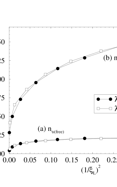
FIG. 1.: The total and free vortex densities vs $1/\xi_{L}^{2}$ for $\lambda=0.0$ and $0.9$. The errors are smaller than the size of the data point symbols.

       

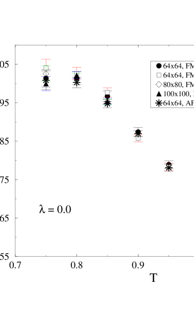
FIG. 2.: Free vortex lifetime vs temperature for $\lambda=0.0$, FM, AFM, and several lattice sizes $L$. The FM* marked cases refer to previous simulations using only Metropolis et al.[35] algorithm in the MC part of the simulations.

       

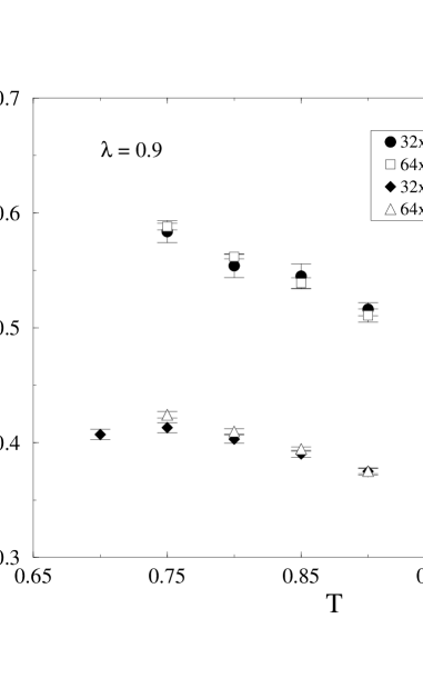
FIG. 3.: Free vortex lifetime vs temperature for $\lambda=0.9$, FM, AFM, and the lattice sizes $L$ indicated.

TABLE I.: Results for the correlation length $\xi_{L}$ for the temperatures, lattice sizes $L\times L$, and anisotropy parameter values $\lambda=0,\ \ 0.9$ considered. The correlation length is in lattice constant units and temperature in $J/k_{B}$.

Temp.		L	$\xi_{L}^{\lambda=0.0}$					$\xi_{L}^{\lambda=0.9}$
0	.7	256						25	.88	${}\pm{}$	0	.96
		128						25	.48	${}\pm{}$	0	.21
0	.75	256	51	.80	${}\pm{}$	0	.5
		64						9	.03	${}\pm{}$	0	.06
0	.8	128	11	.62	${}\pm{}$	0	.36
		32						5	.15	${}\pm{}$	0	.03
0	.85	64	6	.09	${}\pm{}$	0	.20
		32	6	.08	${}\pm{}$	0	.02	3	.58	${}\pm{}$	0	.03
0	.9	32	3	.95	${}\pm{}$	0	.02	2	.77	${}\pm{}$	0	.02
0	.95	32	2	.93	${}\pm{}$	0	.02	2	.29	${}\pm{}$	0	.03
1	.0	32	2	.35	${}\pm{}$	0	.029	1	.88	${}\pm{}$	0	.03
1	.05	32	1	.95	${}\pm{}$	0	.028	1	.69	${}\pm{}$	0	.04
1	.1	32	1	.63	${}\pm{}$	0	.033

TABLE II.: Characteristic times $1/\gamma_{i}=2\xi_{i}/\sqrt{\pi}\bar{u}$, $i=1,\,2$, in the ideal vortex gas theory from published data. The rms vortex velocity $\bar{u}$ and the correlation length $\xi_{2}$ have been obtained from fitting the width of $S^{xx}({\bf q},\omega)$, and $\xi_{1}$ from fitting the integrated intensity.[1, 3, 4]

Temp.	$\bar{u}$	$\xi_{1}$		$\xi_{2}$		$1/\gamma_{1}$	$1/\gamma_{2}$
FM, $\lambda=0.0$, Ref. [1]
0.90	0.84	4	.4	4	.8	5.91	6	.45
1.00	0.91	2	.4	3	.0	2.97	3	.72
1.10	0.91	2	.1	1	.9	2.60	2	.36
AFM, $\lambda=0.0$, Ref. [4]
0.85	1.17	4	.6	9	.02	4.44	8	.70
0.90	0.96	3	.69	5	.28	4.34	6	.21
0.95	1.05	2	.43	4	.35	2.61	4	.67
1.00	1.05	2	.09	3	.28	2.24	3	.52
1.05	1.13	1	.54	3	.17	1.53	3	.16
FM, $\lambda=0.8$, Ref. [3]
0.85	0.39	2	.80	6	.60	8.10	19	.09
0.90	0.47	2	.03	9	.53	4.87	22	.88
0.95	0.43	1	.72	4	.32	4.51	11	.33
AFM, $\lambda=0.8$, Ref. [3]
0.85	1.23	3	.29	6	.87	3.08	6	.30
0.90	1.05	2	.25	3	.74	2.42	4	.01
1.00	0.93	1	.56	2	.26	1.89	2	.74

REFERENCES

- [1] F. G. Mertens, A. R. Bishop, G. M. Wysin, and C. Kawabata, Phys. Rev. Lett. 59, 117 (1987); Phys. Rev. B 39, 591 (1989).
- [2] M. E. Gouvêa, G. M. Wysin, A. R. Bishop, and F. G. Mertens, Phys. Rev. B 39, 11840 (1989); J. Phys. Condens. Matter 1, 4387 (1989); J. Phys. Condens. Matter 2, 1853 (1990).
- [3] A. R. Völkel, A. R. Bishop, F. G. Mertens, and G. M. Wysin, J. Phys. Condens. Matter 4, 9411 (1992).
- [4] A. R. Völkel, G. M. Wysin, A. R. Bishop, and F. G. Mertens, Phys. Rev. B, 44, 10066 (1991);
- [5] F. G. Mertens, A. R. Völkel, G. M. Wysin and A. R. Bishop, in Nonlinear Coherent Structures in Physics and Biology, edited by M. Remoissenet and M. Peyrard (Springer-Verlag, Berlin, 1991).
- [6] A. R. Völkel, F. G. Mertens, G. M. Wysin and A. R. Bishop, J. Magn. Magn. Mater. 104-107, 766 (1992).
- [7] B. A. Ivanov and D. D. Sheka, Phys. Rev. Lett. 74, 404 (1994).
- [8] B. A. Ivanov and A. K. Kolezhuk, Low. Temp. Phys. 21, 275 (1995).
- [9] A.A. Thiele, Phys. Rev. Lett. 30, 230 (1973); J. Appl. Phys. 45, 377 (1974).
- [10] D.L. Huber, Phys. Lett. 76A, 406 (1980); Phys. Rev. B 26, 3758 (1982).
- [11] G. M. Wysin, F. G. Mertens, A. R. Völkel and A. R. Bishop, in proceedings of workshop on “Nonlinear Coherent Structures in Physics and Biology,” (Plenum Press, New York, 1994)
- [12] G. M. Wysin, Phys. Rev. B 54, 15156 (1996).
- [13] D. A. Dimitrov and G. M. Wysin, Phys. Rev. B 53, 8539 (1996).
- [14] N. D. Mermin and H. Wagner, Phys. Rev. Lett. 17, 1133 (1966).
- [15] V. L. Berezinskii, Sov. Phys. JETP 32, 493 (1970).
- [16] J. M. Kosterlitz and D. J. Thouless, J. Phys. C 6, 1181 (1973).
- [17] J. M. Kosterlitz, J. Phys. C 7, 1046 (1973).
- [18] L. J. de Jongh, Magnetic Properties of Layered Transition Metal Compounds, (Dordrecht: Kluwer Academic, 1990).
- [19] L. J. de Jongh, W. D. van Amstel, and A. R. Miedema, Physica 58, 277 (1972).
- [20] K. Kirrakawa, H. Yoshizawa, and K. Ubikashi, J. Phys. Soc. Japan 51, 2151 (1982).
- [21] M. Ain, J. Phys. (Paris) 48, 2103 (1987).
- [22] S. T. Bramwell, M. T. Hutchings, J. Norman, R. Pynn, and P. Day, J. Phys. (Paris) 48, C8, 1435 (1988).
- [23] L. P. Regnault, C. Lartigue, J. F. Legrand, J. Rossat-Mignod, and Y. Henry, Physica B 156-157, 298 (1989).
- [24] J. Rossat-Mignod, P. Burlet, L. P. Regnault, C. Vettier, J. Magn. Magn. Mater. 90/91, 5 (1990).
- [25] P. Gaveau, J. P. Boucher, A. Bouvet, L. P. Regnault, and Y. Henry, J. Appl. Phys. 64, 6228 (1991).
- [26] D. G. Wiesler, H. Zabel, and S. M. Shapiro, Z. Phys. B 93, 277 (1994).
- [27] M. Pomerantz, Surf. Sci. 142, 556 (1984); D. I. Head, B. H. Blott, and D. Melville, J. Phys. (Paris) Colloq. 49, C8-1649 (1988).
- [28] G. M. Wysin, M. E. Gouvêa, A. R. Bishop, and F. G. Mertens, in Computer Simulation Studies in Condensed Matter Physics, D. P. Landau, K. K. Mon and H.-B. Schüttler, eds. (Springer-Verlag, Berlin, 1988).
- [29] G. M. Wysin, (submitted).
- [30] B. A. Ivanov, A. K. Kolezhuk, and G. M. Wysin, Phys. Rev. Lett. 76, 511 (1996).
- [31] G.M. Wysin, M.E. Gouvêa and A.S.T. Pires, (submitted).
- [32] H. G. Evertz and D. P. Landau, Phys. Rev. B 54, 12302 (1996).
- [33] See for example W. H. Press, B. P. Flannery, S. A. Teukolsky, and W. T. Vetterling, Numerical Recipes (Cambridge University Press, 1986) for a particular implementation of the Runge-Kutta method.
- [34] U. Wolff, Phys. Rev. Lett. 62, 361 (1989).
- [35] N. Metropolis, A. W. Rosenbluth, M. N. Rosenbluth, A. H. Teller, and E. Teller, J. Chem. Phys. 21, 1087 (1953).
- [36] M. Creutz, Phys. Rev. D 36, 515 (1987); F. Brown and T. J. Woch, Phys. Rev. Lett. 58, 2394 (1987).
- [37] F. Cooper, B. Freedman, and D. Preston, Nucl. Phys. B210, 210 (1982).
- [38] J.-K. Kim, Europhys. Lett. 28, 211 (1994); Phys. Rev. D 50, 4663 (1994); J.-K. Kim, A. J. F. de Souza, and D. P. Landau, Phys. Rev. E 54, 2291 (1996).
- [39] A. Cuccoli, V. Tognetti, and R. Vaia, Phys. Rev. B 52, 10221 (1995).
- [40] E. Manousakis, Rev. Mod. Phys. 63, 1 (1991).
- [41] U. Wolff, Nucl. Phys. B322, 759 (1989).
- [42] J. Tobochnik and G. V. Chester, Phys. Rev. B 20, 3761 (1979).
- [43] R. Gupta, J. DeLapp, G. G. Batrouni, G. C. Fox, C. F. Baillie, J. Apostolakis, Phys. Rev. Lett. 61, 1996 (1988).
- [44] R. Gupta and C. F. Baillie, Phys. Rev. B 45, 2883 (1992).
- [45] V. Privman, ed., Finite Size Scaling and Numerical Simulation of Statistical Systems, World Scientific Publishing, Singapore (1990).
- [46] J.E.R. Costa and B.V. Costa, Phys. Rev B 54, 994 (1996).