Chaotic enhancement in microwave ionization of Rydberg atoms

Abstract

The microwave ionization of internally chaotic Rydberg atoms is studied analytically and numerically. The internal chaos is induced by magnetic or static electric fields. This leads to a chaotic enhancement of microwave excitation. The dynamical localization theory gives a detailed description of the excitation process even in a regime where up to few thousands photons are required to ionize one atom. Possible laboratory experiments are also discussed.

I Introduction

The pioneering experiment of Bayfield and Koch performed in 1974 [3] attracted a great interest to ionization of highly excited hydrogen and Rydberg atoms in a microwave field [4, 5, 6, 7, 8, 9]. The main reason of this interest is due to the fact that such ionization requires the absorption of a large number of photons (about $20-70$) and can be explained only as a result of the appearence of dynamical chaos and diffusive energy excitation in the corresponding classical system. Indeed the critical border $\epsilon_{c}$ for the microwave field intensity above which classical chaotic motion takes place is given by [4]:

$$\epsilon_{0}>\epsilon_{c}\approx\frac{1}{49{\omega_{0}}^{1/3}}.$$ (1)

Here, $\epsilon$ and $\omega$ are the microwave field strength and frequency, $\epsilon_{0}=\epsilon n_{0}^{4}$ and $\omega_{0}=\omega n_{0}^{3}$ are the rescaled values, and $E_{0}=-1/2n_{0}^{2}$ is the initial unperturbed energy of the atom (see rescaling details below; atomic units are used). It is also assumed that $\omega_{0}\geq 1$ and that the initial orbital momentum $l<(3/\omega)^{1/3}$. For $\epsilon_{0}<\epsilon_{c}$ the electron energy $E$ only performs small oscillations around its initial value and therefore ionization is impossible in the classical system. Above the chaos border instead, the electron’s energy increases in a diffusive way with a diffusion rate per unit time given by [4]:

$$D_{E}=\frac{(\Delta E)^{2}}{\Delta t}\approx 0.5\frac{\epsilon^{2}}{\omega^{4/3}n_{0}^{3}}.$$ (2)

This diffusion leads to electron’s ionization after a typical diffusive time scale $t_{D}\sim E_{0}^{2}/D_{E}$, with $E_{0}=-1/2n_{0}^{2}$ being the initial energy. Such classical diffusive ionization requires many microwave periods ($t_{D}\omega/2\pi\gg 1$) and quantum interference effects can suppress this diffusion leading to quantum localization of chaos [5, 7]. Such dynamical localization of chaos leads to a quantum probability distribution $f_{N}$ exponentially localized in the number of absorbed photons $N_{\phi}=(E-E_{0})/\omega$, namely $f_{N}\propto\exp(-2|N_{\phi}|/\ell_{\phi_{\omega}})$. For the general case of monochromatic field excitation in a complex spectrum the localization length $\ell_{\phi_{\omega}}$, measured in the number of photons, can be determined via the one-photon transition rate $\Gamma\sim D_{E}/\omega^{2}$ and the density of coupled states $\rho_{c}$ [10]:

$$\ell_{\phi_{\omega}}=2\pi\Gamma\rho_{c}=3.33\frac{\epsilon^{2}}{\omega^{10/3}}.$$ (3)

The last equality in the above equation corresponds to the hydrogen case, where $\rho_{c}=n_{0}^{3}$ due to Coulomb degeneracy (which, as is known, is responsible for the appearence of an additional integral on motion [7]). Quite obviously, in case of strong localization, namely when the localization length is less than the number of photons required for ionization, $N_{I}=|E_{0}|/\omega=n_{0}/2\omega_{0}$, the quantum ionization is exponentially small and therefore negligible compared to its classical value. In the opposite case $\ell_{\phi_{\omega}}>N_{I}$, namely above the quantum delocalization border $\epsilon_{q0}$

$$\epsilon_{0}>\epsilon_{q0}=\frac{\omega_{0}^{7/6}}{\sqrt{6.6n_{0}}},$$ (4)

quantum ionization takes place in close to the classical case [7]. We note that the above dynamical localization represents a deterministic analog of the Anderson localization in disordered quasi–one–dimensional chains. In our case the site index corresponds to the photon number $N_{\phi}$, while $N_{I}$ plays the role of the effective sample size.

The above theoretical results have been checked by different groups [6, 8] and more recently reconfirmed in numerical simulations with newly developed algorithms [11, 12]. The predictions of dynamical localization have been also confirmed by laboratory experiments [13, 14, 15]. However, in the mesoscopic solid-state language, the effective “sample size” available in these experiments, corresponding to $N_{I}\approx 20$ was too short to test with sufficient accuracy the theoretical predictions. In fact in this situation one observes significant mesoscopic fluctuations in the ionization border which have been discussed in detail in [8, 9]. While the main structure of these mesoscopic fluctuations can be well described by the quantum Kepler map [16] it is still highly desirable to have much longer “samples” with $N_{I}\geq 100$ to study experimentally the dynamical localization of chaos in more detail. We note that recently the dynamical localization has been also observed in experiments with cold atoms propagation [17]; however, in this situation there are other experimental restrictions.

In order to have larger $N_{I}$ values, one has, either to increase $n_{0}$ or to take $\omega_{0}\ll 1$. However, the first possibility is restricted by experimental conditions where one prefers to have $n_{0}<100$. The second choice leads to a regime close to the static field ionization in which no classical chaos exists; in any case, localization of classically chaotic motion does not take place for $\omega_{0}<<1$. In order to actually have large $N_{I}$ values, it is necessary to take a different approach and work with atoms which are classically chaotic already in the absence of the microwave field. There are two main possibilities to have chaotic Rydberg atoms. One way is to put hydrogen or Rydberg atoms in a magnetic field. In this case, the classical dynamics becomes chaotic when the Larmor frequency is comparable with the unperturbed Kepler frequency [18, 19, 20]. Another possibility is to use Rydberg atoms with quantum defects in a static electric field. Recent investigations have shown that for a sufficiently strong static field the level spacing statistics is similar to the case of random matrix theory (RMT) [21]. From the experimental viewpoint the case with a static electric field is simpler to deal with and in fact can be studied in laboratory experiments similar to [22, 23, 24]. For such atoms the chaos border for the microwave field drops to zero and therefore even at very small microwave field one can expect to see diffusive excitation in energy. In addition, such a diffusion can take place for much lower frequencies with $1/n_{0}\ll\omega_{0}\ll 1$, and this fact allows to increase the values of $N_{I}$ up to few thousands.

The investigation of the interaction of chaotic Rydberg atoms with a microwave radiation is also interesting from another viewpoint. Indeed, it is known that a chaotic structure of eigenstates leads to a strong enhancement of the interaction. In nuclear physics, as was shown by Sushkov and Flambaum [25], this effect leads to an enhancement of weak interaction and parity violation by a factor of thousand or more. Also in the problem of Anderson localization in disordered solid–state systems it has been found that a short range repulsive/attractive interaction between two particles can strongly enhance their propagation [26]. All this indicates that a chaotic structure of Rydberg atoms can strongly increase their interaction with radiation. This should lead to a significant decrease of the quantum delocalization border as compared to the standard case of internally non-chaotic atoms studied in [5, 7]. In fact, the experiments by Gallagher et al. [22, 23] indicated a lower ionization border than for the hydrogen case [9]. The physical mechanism of such ionization, proposed by Gallagher et al. [22, 23], is based on a picture of successive Landau-Zener crossings in a slowly oscillating microwave field. However, the question how such transitions can proceed to high levels was never studied in detail. Moreover, for $\omega>1/n^{4}$ one enters in a multiphoton regime which was not discussed in [22, 23].

Due to the above reasons, the investigation of chaotic enhancement of microwave ionization of Rydberg atoms allows to address a new physical regime in which thousands of photons are required to ionize one atom. Our theoretical and numerical results indeed clearly demostrate the existence of such enhancement and provide a clear physical picture of the ionization process. In section II we discuss the case of atoms in parallel magnetic and microwave fields, while the case of Rydberg atoms in static and microwave fields is analysed in Section III. The main results are discussed in Section IV. Some results have been presented in [27, 28, 29].

II The hydrogen atom in magnetic and microwave fields

The Hamiltonian of a hydrogen atom in parallel microwave and uniform magnetic fields writes

$$\begin{array}[]{c}\displaystyle{H=\frac{p_{\rho}^{2}}{2}+\frac{p_{z}^{2}}{2}+\frac{L_{z}^{2}}{2\rho^{2}}-\frac{1}{\sqrt{\rho^{2}+z^{2}}}+\frac{\omega_{L}L_{z}}{2}+}\cr\cr\displaystyle{\frac{\omega_{L}^{2}}{8}\,\rho^{2}+\epsilon z\sin(\omega t)},\end{array}$$ (8)

where $z$ is the direction of the fields, $\rho=(x^{2}+y^{2})^{1/2}$, $\omega_{L}=B/c=B(T)/B_{0}$ is the cyclotron frequency, $B_{0}=2.35\times 10^{5}T$, $\epsilon$ and $\omega$ are the microwave strength and frequency respectively (atomic units are used). Due to the cylindrical symmetry, the $z$ component of the angular momentum $L_{z}$ is a constant of the motion and here we consider $L_{z}=0$.

The above Hamiltonian, expressed as a function of cartesian coordinates $\{x_{i}\}$, their conjugate momenta $\{p_{i}\}$, the time $t$ and the parameters $L_{z}$, $\omega_{L}$, $\epsilon$, $\omega$ has the property

$$\begin{array}[]{c}\displaystyle{\tilde{H}=H(\{\lambda x_{i}\},\{\lambda^{-1/2}p_{i}\},\lambda^{3/2}t,\lambda^{1/2}L_{z},\lambda^{-3/2}\omega_{L},}\cr\cr\displaystyle{\lambda^{-2}\epsilon,\lambda^{-3/2}\omega)=\lambda^{-1}H(\{x_{i}\},\{p_{i}\},t,L_{z},\omega_{L},\epsilon,\omega).}\end{array}$$ (12)

If we choose $\lambda=1/n_{0}^{2}$, with $E_{0}=-1/2n_{0}^{2}$ the initial energy, the classical dynamics depends on $n_{0}$ only via the scaled variables [7, 18, 19, 20]

$$L_{z}/n_{0},\quad\omega_{L}n_{0}^{3},\quad\epsilon_{0}=\epsilon n_{0}^{4},\quad\omega_{0}=\omega n_{0}^{3}.$$ (13)

The coordinates and momenta scale as $\tilde{x}_{i}=x_{i}/n_{0}^{2}$, $\tilde{p}_{i}=p_{i}n_{0}$ and the rescaled time $\tilde{t}=t/n_{0}^{3}$, up to a factor of $1/2\pi$, counts the number of Kepler periods in the electron motion in the absence of external fields ($\omega_{L}=\epsilon=0$).

In order to study the dynamics of the time–dependent Hamiltonian (8), it is possible to introduce an extended phase space in which the Hamiltonian becomes conservative with respect to a fictitious time $\eta$. The new Hamiltonian writes $K=\tilde{H}+\omega_{0}\tilde{N}$, with $\phi=\omega_{0}\tilde{t}=\omega t$ and $\tilde{N}$ as new classical conjugate variables. The equations of motion for $\phi$ and $\tilde{N}$ are given by

$$\frac{d\phi}{d\eta}=\frac{\partial K}{\partial\tilde{N}}=\omega_{0},\quad\frac{d\tilde{N}}{d\eta}=-\frac{\partial K}{\partial\phi}=-\frac{\partial\tilde{H}}{\partial\phi}.$$ (14)

Notice that $\eta$ is equal to the scaled time $\tilde{t}$ up to an additive constant, and therefore the ordinary Hamilton’s equations follow for the other canonical variables. Since $K$ is a constant of motion, in the quantum case the change of $\tilde{N}$ would give, apart from a $1/n_{0}$ scaling factor, the number of photons $\Delta N$ exchanged by the atom with the field [7]: $\Delta\tilde{N}=-\Delta\tilde{H}/\omega_{0}=-(1/n_{0})(\Delta E/\omega)=-(1/n_{0})\Delta N$.

The singularity of the Hamiltonian (8) at $r=(\rho^{2}+z^{2})^{1/2}=0$ can be removed by introducing the semi–parabolic coordinates $u=(\tilde{r}+\tilde{z})^{1/2}$, $v=(\tilde{r}-\tilde{z})^{1/2}$ and the regularized time $\sigma$, defined as [18, 19, 20]

$$d\eta=d\tilde{t}=(u^{2}+v^{2})\,d\sigma=2\tilde{r}d\sigma,$$ (15)

which changes faster than $\tilde{t}$ near the nucleus and more slowly far from it. The equations of motion generated by the Hamiltonian (8) are then equivalent to the equations of motion generated, with respect to the new time $\sigma$, by the scaled and regularized Hamiltonian

$$\cal{K} =(u^{2}+v^{2})K.$$ (16)

Indeed, for any classical quantity $f(u,v,\phi;p_{u},p_{v},\tilde{N})$, we get

$$\frac{df}{d\sigma}=\frac{df}{d\eta}\,\frac{d\eta}{d\sigma}=\{K,f\}(u^{2}+v^{2}),$$ (17)

where $\{K,f\}$ denotes the Poisson bracket between $K$ and $f$. Thus, if we take $\tilde{N}_{0}=-(1/n_{0})(E_{0}/\omega)$ as initial condition for $\tilde{N}$, the compensated energy $K$ is equal to zero and we obtain

$$\{\cal{K} ,f\}=\{u^{2}+v^{2},f\}K+(u^{2}+v^{2})\{K,f\}=\displaystyle\frac{df}{d\sigma},$$ (18)

that is $\cal{K}$ works as an effective Hamiltonian for the time $\sigma$. For $L_{z}=0$ we have

$$\begin{array}[]{c}\displaystyle{{\cal{K}}=\frac{p_{u}^{2}+p_{v}^{2}}{2}-2+\frac{(\omega_{L}n_{0}^{3})^{2}}{8}u^{2}v^{2}(u^{2}+v^{2})+}\cr\cr\displaystyle{\frac{\epsilon_{0}}{2}\,(u^{4}-v^{4})\sin\phi+\omega_{0}\tilde{N}(u^{2}+v^{2}).}\end{array}$$ (22)

For $\epsilon=0$, $\omega_{0}\tilde{N}=1/2$ and therefore the Hamiltonian (22) represents two harmonic oscillators of unit frequency coupled by the term $\frac{1}{8}\,(\omega_{L}n_{0}^{3})^{2}u^{2}v^{2}\,(u^{2}+v^{2})$ which originates from the diamagnetic interaction. For low scaled magnetic field $\omega_{L}n_{0}^{3}$, the motion is regular and the orbits are quasiperiodic. However, the diamagnetic term has cylindrical symmetry since it depends only on the perpendicular distance $\rho$ from the magnetic field axis. On the contrary, the Coulomb term has spherical symmetry. When these two terms are of comparable magnitude,

$$\frac{1}{\sqrt{\rho^{2}+z^{2}}}\sim\frac{1}{8}\omega_{L}^{2}\rho^{2}$$ (23)

(that gives $\omega_{L}n_{0}^{3}$ of the order of unity), then the competition between different symmetries leads to chaotic motion [18, 19, 20]. In Fig.1 the classical phase space structure is illustrated by the Poincaré surfaces of section. For $\omega_{L}n_{0}^{3}=3$ some islands of stability still exist but their size is small, while for $\omega_{L}n_{0}^{3}=9.2$ no regular structures are visible and the classical motion is dominated by global chaos [18, 19, 20].

Due to this internal chaos, the turn on of the microwave field immediately leads to diffusive energy excitation of the electron, with classical diffusion rate per unit time $D_{B}=<(\Delta E)^{2}>/\Delta t$. From Eq.(8) $\dot{E}=\epsilon z\omega\cos(\omega t)$, with the typical frequencies for the $z$ motion of the order of the Kepler frequency $\omega_{K}=n_{0}^{-3}$ (for $\omega_{L}n_{0}^{3}$ not too large with respect to $1$). For $\omega_{0}\ll 1$, $D_{B}$ can be estimated in quasilinear approximation [27], giving $D_{B}\sim(\epsilon z\omega)^{2}/\omega_{K}$ and then

$$D_{B}\approx\chi_{1}D_{0}\omega_{0}^{2},$$ (24)

where $\chi_{1}$ is a constant to be numerically determined and $D_{0}=\epsilon^{2}n_{0}/2$ is the diffusion rate for $\omega_{L}=0$ and $\omega_{0}=1$ when the microwave intensity is strong enough to induce chaos [7].

For $\omega_{0}\gg 1$, in analogy with the case without magnetic field, the microwave interaction is mainly effective when the electron passes close to the nucleus, where the Coulomb term dominates the diamagnetic term, and therefore, as for the case $\omega_{L}=0$, one has [27]:

$$D_{B}\approx\chi_{2}D_{0}\omega_{0}^{-4/3},$$ (25)

with a constant $\chi_{2}$ again to be numerically determined.

An example of diffusive energy excitation, for scaled frequency $\omega_{0}\ll 1$, is shown in Fig.2. Here $\omega_{L}n_{0}^{3}=3$, so that the motion is chaotic even in the absence of the microwave and therefore a diffusive process occurs even if the microwave intensity is very small.

The frequency dependence of the diffusion rate $D_{B}$ is shown in Fig.3, for $\omega_{L}n_{0}^{3}=3$ and $9.2$. The asymptotic behaviors (both for small and large frequencies) are in agreement with the theoretical estimates (24) and (25) respectively, indicated in the figure by the straight lines, with the coefficients $\chi_{1}$ and $\chi_{2}$ numerically determined. These coefficients depend weakly on $\omega_{L}$, for magnetic field strong enough to induce internal chaos ($\omega_{L}n_{0}^{3}\gtrsim 2$). Below this value the internal motion becomes integrable and for low enough $\epsilon_{0}$ diffusion drops to zero, as demonstrated in the insert of Fig.3 (see also [27]).

The classical diffusive process will lead the electron to ionization in a time $t_{I}\approx E_{0}^{2}/D_{B}$, with $E_{0}=-1/2n_{0}^{2}$ the initial electron energy. In the quantum case, for $n_{0}\gg 1$ the time evolution initially follows the classical diffusion. The excitation proceeds via a chain of one–photon transitions, which eventually brings the electron into continuum. However, if the ionization time is sufficiently large, quantum interference effects may suppress the diffusive excitation leading to dynamical localization in the number of photons.

In order to check this possibility we numerically analyzed the quantum dynamics [28], following the wave packet evolution in the eigenstates basis of the magnetic field problem with $\epsilon=0$.

To obtain these eigenstates at $\epsilon=0$ in a given energy window around the initially excited level with eigenenergy $E_{\lambda_{0}}\approx E_{0}$, we diagonalized the Hamiltonian in a parabolic Sturmian basis [5, 11]. This basis is well suited since it is complete and discrete and can efficiently reproduce both the bound and continuum states of the hydrogen atom. In addition, all the Hamiltonian matrix elements can be expressed in a simple analytical form and strong selection rules exist for the parabolic quantum numbers $n_{1}$, $n_{2}$ ($\Delta n_{i}=0,\pm 1,\pm 2$ for $i=1,2$). A minor disadvantage of dealing with a Sturmian basis is associated with its nonorthogonality. Due to this fact, we had to solve a generalized eigenvalue problem of the type $H\psi_{i}=E_{\lambda_{i}}S\psi_{i}$, where also the overlap matrix $S$ has strong selection rules ($\Delta n_{i}=0,\pm 1$ for $i=1,2$). As a result the matrices $H$ and $S$ are very sparse. To study the time evolution we used up to $1250$ eigenstates of the above generalized eigenvalue problem. In order to obtain a good convergence of these $1250$ eigenvectors and eigenvalues we had to diagonalize matrices of size larger than $13,000$. For these reasons the use of an efficient Lanczos algorithm [30] has been crucial. The time evolution was computed by a split–step metod, similar to the one used in [5].

In our computations, we considered as initial state an eigenstate at $\epsilon=0$ with eigenenergy $E_{\lambda_{0}}\approx E_{0}=-1/2n_{0}^{2}$ and the time evolution in the microwave field was followed up to $\tau=200$ microwave periods. The parameters were varied in the intervals $0.05\leq\omega_{0}\leq 3$, $0.002\leq\epsilon_{0}\leq 0.04$, $40\leq n_{0}\leq 80$, for $\omega_{L}n_{0}^{3}=3$ and $9.2$.

In this quasiclassical regime the quantum energy excitation has initially a diffusive character (see the insert of Fig.4) and therefore it is possible to compute a quantum diffusion coefficient $D_{B}^{(q)}$ from a linear fit, for the few first microwave periods, of the wave packet energy square variance $<(\Delta E)^{2}>$ vs. time. Fig.4 shows that quantum and classical diffusion coefficients are similar over a wide range of frequencies ($0.05\leq\omega_{0}\leq 3$ for $n_{0}=60$). This demonstrates that quantum dynamics mimics, for a finite interaction time, the classical excitation.

In the quasiclassical regime, the one–photon transition rate $\Gamma_{B}$ can be related to the classical diffusion rate [10] as $\Gamma_{B}=D_{B}/\omega^{2}$. Indeed the change in energy produced by a one–photon transition is $\Delta E=\pm\omega$ and $\Gamma_{B}$ measures the number of such transitions per unit time. Therefore, the ratio $\Gamma_{B}/\Gamma_{0}$, where $\Gamma_{0}=D_{0}n_{0}^{6}$ is the transition rate for the chaotic case at $\omega_{L}=0$ and $\omega_{0}=1$, is equal to

$$\frac{\Gamma_{B}}{\Gamma_{0}}=\frac{D_{B}}{D_{0}\omega_{0}^{2}}.$$ (26)

This result is remarkable as it relates the quantum transition rate to a classical characteristic of motion, namely the diffusion coefficient. In order to check the above estimate, $\Gamma_{B}$ was numerically evaluated according to Fermi’s Golden Rule:

$$\begin{array}[]{c}\displaystyle{\Gamma_{B}=\frac{\pi}{2}\,\epsilon^{2}\sum_{m\neq n}|z_{mn}|^{2}\{\delta(E_{\lambda_{m}}-E_{\lambda_{n}}+\omega)+}\cr\cr\displaystyle{\delta(E_{\lambda_{m}}-E_{\lambda_{n}}-\omega)\},}\end{array}$$ (30)

with $z_{mn}$ matrix elements of $z$ between the eigenstates at $\epsilon=0$ with eigenenergies $E_{\lambda_{m}},E_{\lambda_{n}}$. For the numerical computation, the Dirac delta function in Eq.(30) was substituted by a Lorentzian function: $\delta(x)\to f(x)=(1/\pi)(\tilde{\epsilon}\,/(x^{2}+\tilde{\epsilon}^{2}))$, with $\tilde{\epsilon}$ of the order of the level spacing. The validity of the classical–quantum correspondence (26) is confirmed in Fig.5, for $n_{0}=40,60,80$ and $0.05\leq\omega_{0}\leq 3$.

Even if initially the interaction with the microwave field results in a quantum diffusive excitation, quantum interference effects can suppress the diffusive behavior before ionization takes place. In this case, the diffusive broadening of the quantum probability distribution over unperturbed levels stops. The corresponding localization length (measured in number of absorbed photons) $\ell_{B}$ is proportional to the one–photon transition rate $\Gamma_{B}$ and to the density of coupled states $\rho_{B}$: $\ell_{B}=2\pi\Gamma_{B}\rho_{B}$ [10]. For the chaotic case at $\omega_{L}=0$ and $\omega_{0}=1$ the localization length is $\ell_{\phi}=3.3\epsilon_{0}^{2}n_{0}^{2}=2\pi D_{0}n_{0}^{6}\rho_{0}=2\pi\Gamma_{0}\rho_{0}$, where $\rho_{0}=n_{0}^{3}$ is the density of coupled states [7]. Actually, without the magnetic field there is an additional approximate integral of motion, related to Coulomb degeneracy, and therefore the density of coupled states $\rho_{0}$ is by a factor $n_{0}$ smaller than the number of levels per unit energy interval $n_{0}^{4}$ [7]. Therefore from the above expressions and Eq.(26) we get [27, 28]

$$\ell_{B}=\ell_{\phi}\frac{D_{B}}{D_{0}\omega_{0}^{2}}\frac{\rho_{B}}{\rho_{0}}.$$ (31)

This result provides a theoretical formula for the the quatum localization length, which involves only classical characteristics of motion, namely the classical diffusion coefficient and the density of coupled states. The latter is related, in the quasiclassical regime, to the phase space structure (see below Eqs.(32)–(33)). The estimate (31) is valid for $\ell_{B}>1$, namely in the quasiclassical regime, in which a large number of photons is absorbed and a large number of levels is excited. Moreover, the microwave frequency should be larger than the average level spacing ($\omega\rho_{B}>1$); otherwise, levels would move adiabatically in time leaving no room for diffusive energy growth [7].

For $\omega_{L}n_{0}^{3}$ sufficiently large, the internal motion is chaotic: as a consequence, Coulomb degeneracy is removed and the density of coupled states $\rho_{B}\sim n_{0}^{4}$. More precisely, $\rho_{B}=0.34n_{0}^{4}$ (for $\omega_{L}n_{0}^{3}=3$, $n_{0}=60$) and $\rho_{B}=0.14n_{0}^{4}$ (for $\omega_{L}n_{0}^{3}=9.2$, $n_{0}=60$) (see Fig.6). The density follows the dependence $\rho_{B}\propto 1/\omega_{L}$. This is related to the fact that the diamagnetic term is identical to a two–dimensional harmonic oscillator in the $x-y$ plane. Indeed for a harmonic oscillator the spacing between levels is proportional to the frequency (here represented by $\omega_{L}$) and therefore their density scales with $\omega_{L}^{-1}$. This result is confirmed by a quasiclassical computation of the density of states (see the insert of Fig.6). Here the number $\Omega(E)$ of quantum states having energy less than $E$ is related to the corresponding volume in phase space

$$\displaystyle{\Omega(E)=\frac{1}{(2\pi)^{2}}\int_{H<E}\,d\rho dzdp_{\rho}dp_{z},}$$ (32)

where the Hamiltonian $H$ is taken at $\epsilon=0$. The density of states is

$$\rho_{B}=\frac{d\Omega(E)}{dE}=n_{0}^{4}\,\frac{d\tilde{\Omega}(\tilde{E})}{d\tilde{E}},$$ (33)

where the volume in the scaled phase space is defined as

$$\displaystyle{\tilde{\Omega}(\tilde{E})=\frac{1}{(2\pi)^{2}}\int_{\tilde{H}<\tilde{E}=-\frac{1}{2}}\,dudvdp_{u}dp_{v},}$$ (34)

with

$$\displaystyle{\tilde{H}=\frac{p_{u}^{2}+p_{v}^{2}}{2(u^{2}+v^{2})}-\frac{2}{u^{2}+v^{2}}+\frac{(\omega_{L}n_{0}^{3})^{2}}{8}\,u^{2}v^{2}.}$$ (35)

According to the results of Fig.6 such semiclassically determined density of states is in a good agreement with the results obtained by direct diagonalization of hydrogen in magnetic field.

According to the estimate (31) and differently from the zero magnetic field case, the localization length $\ell_{B}$ is non homogeneous in the number $N_{\phi}$ of absorbed photons. Indeed, from equations (24) and (25) we get $\ell_{B}\sim n_{0}^{11}\sim(N_{I}-N_{\phi})^{-11/2}$ for $\omega_{0}\ll 1$ and $\ell_{B}\sim n_{0}\sim(N_{I}-N_{\phi})^{-1/2}$ for $\omega_{0}\gg 1$ [27], with $N_{I}=n_{0}/2\omega_{0}$ the number of photons required for ionization and $N_{\phi}=N-N_{0}$, where $N_{0}=E_{0}/\omega$. However, for $\ell_{B}\ll N_{I}$ this effect is not important and the quasistationary distribution is exponentially localized in the photon number $N_{\phi}$. As for the case of hydrogen in a microwave field only [7], the probability distribution over unperturbed levels ($\epsilon=0$) displays a chain of equidistant peaks in energy. The probability amplitudes in a one–photon interval decay esponentially with the photon number: $\psi_{N}\propto\exp(-|N-N_{0}|/\ell_{B})$.

The value of the localization length $\ell_{B}$ is strongly enhanced compared to the length $\ell_{\phi_{\omega}}=3.3\epsilon_{0}^{2}n_{0}^{2}/\omega_{0}^{10/3}$ [7] at $\omega_{L}=0$ and $\omega_{0}>1$. Actually, for a strong enough scaled magnetic field, Coulomb degeneracy is removed and the eigenfunctions $\psi$, when developed on the basis of the hydrogenic eigenfunctions $\varphi$, have a large number of randomly fluctuating components, increased by a factor $M=\rho_{B}/\rho_{0}$:

$$\psi_{i}\approx\sum_{k=1}^{M}c_{ik}\varphi_{k},$$ (36)

with $c_{ik}\sim 1/\sqrt{M}$ due to normalization condition. Because of this, the external microwave perturbation $V$ couples the eigenstates with typical interaction matrix elements

$$V_{int}=\langle\psi_{j}|V|\psi_{i}\rangle\approx\sum_{k,l=1}^{M}c_{jl}^{*}c_{ik}\langle\varphi_{l}|V|\varphi_{k}\rangle.$$ (37)

Due to selection rules for $V$ in the hydrogenic basis, $V_{int}$ is the sum of order $M$ uncorrelated terms and is therefore reduced by a factor $1/\sqrt{M}$ in comparison with the case without magnetic field, whereas the spacing $\Delta E$ between nearest neighbors levels in the spectrum scales as $1/M$. Thus, the admixture factor

$$\eta\sim V_{int}/\Delta E\sim\sqrt{M}\sim\sqrt{n_{0}}$$ (38)

is strongly enhanced, for high $n_{0}$ values, in comparison with the zero magnetic field case. As a result, the localization length $\ell_{B}$, which is proportional to $\eta^{2}$, is increased [28] by a factor

$$\ell_{B}/\ell_{\phi_{\omega}}\sim\chi_{2}\rho_{B}/\rho_{0}\sim M\sim n_{0}.$$ (39)

A similar effect was discussed for two interacting particles in a disordered solid state system [26]: the interaction allows the two particles to propagate coherently on a distance much larger than one–particle localization length. The statistical enhancement effect is quite general and takes place in different pysical problems: actually this effect was first studied for the weak interaction parity–breaking in the scattering of polarized neutrons on complex nuclei [25]. In the compound nucleus the level spacing is typically $\Delta E\approx 1$ eV, whereas the typical energy scale due to the strong interaction is $\Delta E_{0}\approx 1$ MeV. As a consequence, the number of principal components of the eigenfunctions in the one-particle basis is $M\approx 10^{6}$ and therefore the admixture factor between states of opposite parity is enhanced by a factor $\sqrt{M}\approx 10^{3}$ compared to a usual parity breaking admixture of the order $10^{-7}$.

The condition $\ell_{B}=N_{I}$ allows to determine the quantum delocalization border [27, 28]:

$$\epsilon_{q}=\frac{1}{n_{0}}\sqrt{\frac{D_{0}\omega_{0}^{2}}{6.6D_{B}}\,\frac{\rho_{0}n_{0}}{\rho_{B}\omega_{0}}}.$$ (40)

For $\epsilon_{0}>\epsilon_{q}$ localization effects become unimportant and diffusive ionization close to the classical case takes place. For $\omega_{0}\gg 1$ this border is $(\chi_{2}n_{0}/\omega_{L}n_{0}^{3})^{1/2}$ times smaller than the quantum delocalization border at zero magnetic field [7] $\epsilon_{q0}=\omega_{0}^{7/6}/\sqrt{6.6n_{0}}$. For $\omega_{0}\ll 1$ the border is given by $\epsilon_{q}=(\omega_{L}n_{0}^{3}/6.6\chi_{1}\omega_{0})^{1/2}/n_{0}$, which remains well below the ionization border for a static electric field in the presence of a parallel magnetic field. Since the localization length is non homogeneous in the number of absorbed photons and becomes larger near the ionization border, the actual value of the delocalization border $\epsilon_{q}$ will be slightly decreased as compared to (40).

The above dynamical localization theory was tested by detailed numerical simulations of quantum evolution. The probability distribution $f_{\lambda}$ over the eigenstates at $\epsilon=0$ for the localized case is shown in Figs.7,8 as a function of the number of absorbed photons $N_{\phi}=(E_{\lambda}-E_{0})/\omega$. In order to suppress fluctuactions this probability was averaged over $20$ microwave periods. To find the numerical value $\ell_{BN}$ of the localization length we first computed the probability $f_{N}$ in each one–photon interval around integer values of $N_{\phi}$. Then the least square fit with $f_{N}\sim\exp(-2N_{\phi}/\ell_{BN})$ for $N_{\phi}\geq 0$ allows to determine $\ell_{BN}$. The quantum distribution at $\omega_{0}=0.2$ (Fig.8(b)) starts to deviate from the exponential profile for $N_{\phi}>60$ and a plateau appears. This can be related to the fact that localization length is non homogeneous in the number of absorbed photons ($\ell_{B}\sim(N_{I}-N_{\phi})^{-11/2}$ for $\omega_{0}\ll 1$). In the figures also the classical distribution, normalized to one–photon interval, is shown. This distribution was obtained by numerical solution of Hamilton equations with $1000$ trajectories initially distributed microcanonically on the energy surface at energy $E_{0}$. The comparison of the probability distributions at different times ($80\leq\tau\leq 100$ in Figs.7(a),8(a) and $180\leq\tau\leq 200$ in Figs.7(b),8(b)) shows that the quantum case is well localized over a quasistationary distribution. Its profile does not change significantly by increasing the interaction time, apart from a slight increase in the tail. We attribute the decrease in the probability decay at large $N_{\phi}>0$ to the growth of the diffusion rate $D_{B}$ when $\omega_{0}$ approaches $1$ from below (see Fig.3).

These distributions, together with the time dependence of the square variance of the photon number $<(\Delta N_{\phi})^{2}>$ (see Fig.9) demonstrate how the quantum–mechanical energy diffusion is strongly suppressed in comparison with the classical case.

The numerically obtained localization lengths $\ell_{BN}$ are presented Fig.10, for two fixed values of $\epsilon_{0}$ and different $\omega_{0}$ in the range $0.05\leq\omega_{0}\leq 3$. Since $n_{0}=60$, the number of photons required for ionization goes from $N_{I}=10$ to $N_{I}=600$. The straight line, corresponding to $\ell_{BN}=\ell_{B}$, demonstrates the fairly good agreement between numerical data and dynamical localization theory over a wide range of parameters (the localization length changes by two orders of magnitude).

Finally, Figs.11,12 show that the excitation at $\omega_{L}n_{0}^{3}=3$ is much stronger than at zero magnetic field, due to the chaotic enhancement of electron’s interaction with the microwave field. Since the condition for the transition to chaotic dynamics at zero magnetic field is given by [5, 7] $\epsilon_{0}>\epsilon_{c}=1/49\omega_{0}^{1/3}$, the case of Fig.11 (that corresponds to Fig.10 in [7]) is above the chaos threshold ($\epsilon_{0}>\epsilon_{c}=0.015$). However the quantum distribution at $\omega_{L}=0$ clearly demonstrates exponential localization of diffusive excitation since $\epsilon_{0}<\epsilon_{q0}=0.14$. On the contrary, for $\omega_{L}n_{0}^{3}=3$ we are above the delocalization border ($\epsilon_{0}>\epsilon_{q}=0.016$) and thus numerical results show a good agreement between classical and quantum distributions. The quantum and classical square variance of the photon number are shown in Fig.12. In the absence of the magnetic field, the localization of the quantum motion after a few microwave periods is evident; on the contrary, for $\omega_{L}n_{0}^{3}=3$ the quantum square variance follows the classical one and starts to deviate only for $\tau>20$ because of the finite size of the basis.

III Rydberg atoms in static electric and microwave fields

Another way to study the microwave interaction in an intrinsically chaotic atomic system is to consider alkali Rydberg atoms in a static electric field; this case is interesting as it is more suitable for laboratory experiments.

The Hamiltonian of a hydrogen atom in a static electric field is separable in parabolic coordinates and thus the classical motion is integrable. On the contrary, in alkali atoms the valence electron moves in an attractive potential in which the $1/r$ dependence is modified near the origin due to the charge distribution of the inner electrons, which form a core of size a few Bohr radius. Due to precession in a static electric field, the electron always collides with the core. This fact prevents the separation of variables and the motion becomes chaotic for certain field and energy values [21].

The potential within the many–electron core region can be reasonably approximated by a one–electron spherically symmetric model [31]:

$$V_{c}(r)=-\frac{Z-1}{r}\exp(-\alpha_{1}r)-\alpha_{2}\exp(-\alpha_{3}r),$$ (41)

where $Z$ is the nuclear charge and the parameters $\alpha_{i}$ $(i=1,2,3)$ are numerically determined so as to reproduce quantum defects, that characterize the ionic core of alkali atoms in quantum mechanics. In this way, the overall potential $V(r)=-1/r+V_{c}(r)$ complies with the two conditions $V(r)\sim-Z/r$ (for $r\to 0$, where the core fails to screen the nuclear charge) and $V(r)\sim-1/r$ (for $r\to\infty$, where due to the screening the valence electron feels only a unit charge). Even if different core potential forms could reproduce quantum defects, both classical and quantum properties of the system are sensitive only to the size of these defects, not to details of the core.

In the quantum case, the core potential $V_{c}(r)$ introduces a phase shift $\pi\delta_{l}$ in the radial wave function. The electron energy is then given by $E_{nl}=-1/2(n-\delta_{l})^{2}$, namely the effective principal quantum number becomes $n^{\star}=n-\delta_{l}$, where the quantum defect $\delta_{l}$ depends on the orbital momentum $l$ but changes only weakly with the energy $E$. Since the size of the core is small only the quantum defects for low angular momentum values ($l<3$) are significantly different from zero.

At the ionization threshold, the quantum defects $\delta_{l}$ are given, in quasiclassical approximation, by the action difference in the nonhydrogenic and hydrogenic radial motion between turning points [32]:

$$\begin{array}[]{c}\displaystyle{\delta_{l}=\frac{\sqrt{2}}{\pi}\lim_{R\to\infty}\left[\int_{r_{0c}}^{R}\,\sqrt{\frac{1}{r}-V_{c}(r)-\frac{(l+1/2)^{2}}{2r^{2}}}\,dr\right.}\cr\cr\displaystyle{-\left.\int_{r_{0}}^{R}\,\sqrt{\frac{1}{r}-\frac{(l+1/2)^{2}}{2r^{2}}}\,dr\,\right].}\end{array}$$ (45)

In this formula, $l(l+1)$ has been replaced by $(l+1/2)^{2}$ so that quasiclassical approximation remains valid also for small angular quantum numbers [33]. The turning point for the hydrogenic part is $r_{0}=(l+1/2)^{2}/2$, while for the nonhydrogenic part we obtain $r_{0c}$ as the root of $V(r_{0c})+(l+1/2)^{2}/2r_{0c}^{2}=0$. The parameters $\alpha_{i}$ were fixed in order to reproduce the most important quantum defects $\delta_{0},\delta_{1},\delta_{2}$. For Li we assumed $\delta_{0}=0.4$, $\delta_{1}=0.04$, $\delta_{2}=0$; for Na $\delta_{0}=1.35$, $\delta_{1}=0.85$, $\delta_{2}=0.01$; for Rb $\delta_{0}=3.14$, $\delta_{1}=2.65$, $\delta_{2}=1.35$; we always considered $\delta_{l>2}=0$ [34]. Typical values of the $\alpha_{i}$ parameters are quite different from those given in Tab.1 of [31], probably because in that case these parameters were optimized so as to directly reproduce the energy levels. In any case this difference is not important in evaluating the quantum defects, that can be reproduced from Eq.(45) with $\alpha_{i}$ parameters taken from [31] with a negligible error.

The classical Hamiltonian for alkali atoms in parallel static electric field $\epsilon_{s}$ and microwave field $\epsilon\sin(\omega t)$, both in the $z$–direction, writes as

$$H=\frac{p^{2}}{2}-\frac{1}{r}+V_{c}(r)+\epsilon_{s}z+\epsilon z\sin(\omega t).$$ (46)

The scaling property expressed by Eq.(12) remains valid, provided that also the static field and the core potential parameters are scaled as $\epsilon_{s0}\equiv\epsilon_{s}n_{0}^{4}$, $\alpha_{i0}\equiv\alpha_{i}n_{0}^{2}$ ($i=1,\ldots,3$). In other words, differently from the case of hydrogen, the problem depends separately on $\epsilon_{s}$ and $n_{0}$ and not only on the scaled parameter $\epsilon_{s0}$. As a matter of fact, the transformation $\alpha_{i}\to\alpha_{i0}=\alpha_{i}n_{0}^{2}$ changes the rescaled core size.

The study of the classical dynamics of the above problem was done in a similar way to the case of the hydrogen atom in magnetic and microwave fields. The system was studied in an extended phase space that includes the time as a new canonical variable and the Coulomb singularity at $r=0$ was removed by the introduction of the semi–parabolic coordinates $u,v$ and the regularized time $\sigma$ (Eq.(15)). For simplicity’s sake, we considered only the case with $z$–component of the angular momentum $L_{z}=0$.

For $\epsilon=0$, due to the core effects, we have a transition from regular to chaotic motion by increasing the static field $\epsilon_{s0}$ [21]. However, the nature of chaotic dynamics in this case is qualitatively different from the case of diamagnetic hydrogen. In the latter case, the irregular motion is due to the competition of the spherical Coulomb interaction, that dominates near the nucleus, and the cylindrical diamagnetic interaction, that dominates at large distances. In the former case instead, the chaotic motion arises from the presence of a core, which is small compared to the typical size of Rydberg atoms. Fig.13 shows that the phase space remains dominated by orbits which jump between different tori of the Coulomb problem. A trajectory follows a torus of the hydrogenic system until it encounters the core region where it is scattered on a different torus. As a result a single trajectory is able to explore most of the phase space energetically accessible to it. The lobes near $v=0$ in the Poincaré surface of section in Fig.13 are due to the attractive core, which allows larger values of the momentum for a given energy.

This chaotic motion affects also the quantum energy level spacing statistics [35]. For integrable systems the level spacing statistics has generally the Poisson form $P(s)=\exp(-s)$, with $s$ the spacing between two consecutive levels, normalized to the local mean level spacing. For systems that display chaotic classical motion the distribution $P(s)$ is described by the Random Matrix Theory (RMT). For a number of chaotic systems, with time reversal symmetry, the energy level statistics has been found in agreement with the predictions of the Gaussian orthogonal ensemble of random matrices, with $P(s)$ given by the Wigner–Dyson distribution

$$P(s)=\frac{\pi}{2}\,s\exp(-\frac{\pi}{4}s^{2}).$$ (47)

A Wigner-Dyson distribution of level spacings has been seen in the Li atom in a static electric field strong enough to induce classical chaos [21]. In Fig.14 the normalized nearest neighbor distribution $P(s)$ is shown for $\epsilon_{s0}=0.02$ at $n_{0}=60$, in the range $55\leq n\leq 72$. The hydrogen displays nearly Poissonian behavior while for Rb, in which quantum defects are large, $P(s)$ is close to the RMT results. The case of Na demonstrates a weaker level repulsion than Rb, while Li, which has smaller quantum defects, presents a distribution rather close to the Poisson case.

The energy levels for alkali atoms in a static electric field (the so–called Stark levels) were obtained by matrix diagonalization in a spherical hydrogenic basis; quantum defects were introduced simply in the alkali energy levels (for angular momentum $l<3$), while dipole matrix elements were taken as in the hydrogen case. This approach is valid outside the ionic core, where $V(r)$ is essentially hydrogenic and so is particularly well suited for Rydberg states, in which the electron mainly remains far from the nucleus. The off–diagonal dipole matrix elements for the $z$ operator decrease rapidly with the difference in energy between initial and final states. As a result, Stark eigenvalues and eigenvectors in a given energy window can be obtained by diagonalization of Hamiltonian matrices of limited size around this region. A limitation of the method is that only bound states are included in the basis set and increasingly large matrices must be used to obtain convergence as the static field ionization border $\epsilon_{s}n^{4}=0.13$ is approached.

The number of mixed hydrogenic states can be characterized by the inverse participation ratio

$$\xi_{\lambda_{i}}=(\sum_{n,l}|c_{\lambda_{i}}(n,l)|^{4})^{-1},$$ (48)

where $c_{\lambda_{i}}(n,l)$ are the coefficients of the expansion of the Stark eigenstate with energy $E_{\lambda_{i}}$ on the spherical basis. Fig.15 shows how the inverse participation ratio $\xi$ (obtained averaging $\xi_{\lambda_{i}}$ in one–shell intervals $E(n-1/2)\leq E_{\lambda_{i}}\leq E(n+1/2)$, with $E(x)\equiv-1/2x^{2}$) increases with the energy for a given static field or equivalently (in the insert) with the field for a given energy. As a result, more and more shells are mixed moving to the saddle point $\epsilon_{s0}=0.13$ and chaotic properties become stronger. For $\epsilon_{s0}=0.02$, $n_{0}=60$, $\xi\approx 75$ and this indicates that eigenfunctions are significantly spread over different shells.

When the microwave field is turned on, the internal chaos leads to diffusive energy excitation in the classical dynamics, with energy diffusion rate per unit time $D_{c}=<(\Delta E)^{2}>/\Delta t$. As for the hydrogen atom in static electric and microwave fields, the rate $D_{c}$ can be compared with the diffusion rate $D_{0}$ for hydrogen with only the microwave field present and at $\omega_{0}=1$. Again the asymptotic behaviors $D_{c}=\chi_{1}D_{0}\omega_{0}^{2}$ (for $\omega_{0}\ll 1$) and $D_{c}=\chi_{2}D_{0}\omega_{0}^{-4/3}$ (for $\omega_{0}\gg 1$) are expected. This is confirmed by Fig.16, that shows the frequency dependence of the scaled diffusion rate $D_{c}/D_{0}$ for Rb, Na and Li at $\epsilon_{s0}=0.02$, $\epsilon_{0}=0.005$, $n_{0}=60$. The core potential parameters $\alpha_{i}$ are not changed with the initial level $n_{0}$. As a result, the dependence on the initial energy or on $n_{0}$ can no longer be eliminated by classical rescaling. However the classical scaling rule remains a useful approximation since $D_{c}/D_{0}$ varies very slowly with $n_{0}$ for Rydberg atoms (for Rb at $\epsilon_{s0}=0.02$, $\epsilon_{0}=0.005$, $\omega_{0}=0.1$, $D_{c}/D_{0}$ remains between $0.019$ and $0.023$ for $20\leq n\leq 80$). This fact can be understood by taking into account that only for low $l$ values the electron collides with the core. The energy diffusion rate is therefore determined by the frequency of these collisions, which is determined by the frequency of classical precession in $l$, namely by the scaled Stark frequency $\omega_{s0}=3\epsilon_{s0}$, independently from $n_{0}$. In other words, the dimensions of the core play no important rôle for the classical diffusion rate.

Fig.16 presents some other interesting features: a sharp resonant peak for $\omega_{0}=1$ and a plateau for $0.02\leq\omega_{0}\leq 0.4$. This latter characteristic is due to the fact that core collisions, that are responsible for energy diffusion, occur at the Stark frequency $\omega_{s0}$, independently from $\omega_{0}$. This fact is also illustrated in the insert of Fig.16: for very low microwave intensity ($\epsilon_{0}=0.0005\ll\epsilon_{s0}$) and for $\omega_{0}=0.1$ the diffusion coefficient grows with the static field $\epsilon_{s0}$, while for $\epsilon_{0}=0.005$, when $\epsilon_{s0}<\epsilon_{0}$, the microwave field dominates the angular momentum precession and the dependence of $D_{c}/D_{0}$ on $\epsilon_{s0}$ becomes rather weak.

The peak at $\omega_{0}=1$ in Fig.16 is due to the resonance between Kepler and microwave frequency. Fig.17 shows that the diffusion rate drops abruptly as the electron goes out of the resonance (for $\epsilon_{0}=0.005$ this happens after approximately $10$ microwave periods). Such sharp change of the diffusion rate was observed only near the main resonance $\omega_{0}=1$, while for other integer values of $\omega_{0}$ our studies did not indicate any sharp change.

To study diffusion in the quantum case we considered the initial wavefunction at $t=0$ as an eigenstate of the Hamiltonian (46) at $\epsilon=0$ with eigenenergy $E_{\lambda_{0}}\approx E_{0}=-1/2n_{0}^{2}$ [29]. As in the case of the hydrogen atom in magnetic and microwave fields, the quantum dynamics was followed by a split-step method, similar to the one described in [5]. The quantum diffusion rate $D_{q}$ was obtained by a linear fit of the energy square variance $<(\Delta E)^{2}>$ vs. time for the first few microwave periods. The classical–quantum comparison for the scaled diffusion coefficients $D_{c}/D_{0}$ and $D_{q}/D_{0}$ (see Fig.18) shows a quantitative difference. This is due to the fact that only low angular momentum values contribute to the diffusion and so purely quantum effects can be expected. In addition, the influence of the ionic core is stronger in classical mechanics because trajectories can penetrate in arbitrarily small regions in the phase space. On the contrary, quantum mechanics tends to smooth over such regions. Apparently this is the reason for which classical diffusion rate is sistematically larger than the corresponding quantum value.

Due to quantum interference effects, the above diffusive excitation may eventually stop before ionization. The resulting quasistationary distribution is characterized by an exponential decay in the number of absorbed photons, with a localization length $\ell_{q}$ proportional to the one–photon transition rate $\Gamma_{q}$ and to the density of coupled states $\rho_{c}$: $\ell_{q}=2\pi\Gamma_{q}\rho_{c}$ [10]. The rate is given by $\Gamma_{q}=D_{q}/\omega^{2}$ and since the internal motion is chaotic the density of coupled states is $\rho_{c}=n_{0}^{4}$. This leads to [29]:

$$\ell_{q}=\ell_{\phi}\frac{D_{q}}{D_{0}\omega_{0}^{2}}n_{0},$$ (49)

where, as in Eq.(31), $\ell_{\phi}=3.3\epsilon_{0}^{2}n_{0}^{2}$ and the conditions $\ell_{q}>1$, $\omega\rho_{c}>1$ must be satisfied.

In order to check the theoretical prediction (49), the quantum evolution of an eigenstate with eigenenergy $E_{\lambda_{0}}\approx-1/2n_{0}^{2}$, and $n_{0}=60$ was followed up to $200$ microwave periods in the Stark basis for $\epsilon_{s0}=0.02$. The total basis size was up to $1150$ states. The system parameters were varied in the intervals $0.003\leq\epsilon_{0}\leq 0.03$, $0.02\leq\omega_{0}\leq 2$, which corresponds to $15\leq N_{I}\leq 1500$.

Typical examples of stationary distributions for Rb at $\omega_{0}=0.08$ and $n_{0}=60$ are shown in Fig.19. In order to determine the numerical value $\ell_{qN}$ of the localization length, we first computed the total probability $f_{N}$ in each one–photon interval. Then the least square fit with with $f_{N}\sim\exp(-2N_{\phi}/\ell_{qN})$ allows to determine $\ell_{qN}$. In Fig.19 the numerical localization length $\ell_{qN}$ agrees with the theoretical $\ell_{q}$ value (Eq.(49)) for $\epsilon_{0}=0.005$. The figure also shows how quantum excitation is strongly suppressed in comparison with the classical case. For a smaller microwave intensity ($\epsilon_{0}=0.002$) the fit in the interval $0\leq N_{\phi}\leq 20$ gives $\ell_{qN}=3.7$, whereas the fit for the tail ($N_{\phi}\geq 50$) shows a much slower decay, with $\ell_{qN}=28$. We checked that this slope change is not affected by the variation of the basis size and integration step. This change in the probability decay at large $N_{\phi}$ can be attributed to a significant change in the eigenstate structure in a static electric field when one approaches the saddle point behind which tunneling takes place. Indeed according to the results shown in Fig.15 a Stark eigenstates for higly excited levels projects on a larger number of hydrogenic levels. Additional investigations are required for a better understanding of this effect.

The comparison of the numerically obtained localization lengths $\ell_{qN}$ vs. the theoretical estimates $\ell_{q}$ confirms the predictions of Eq.(49) (see Fig.20 for Rb and Na at a fixed $\epsilon_{0}$ value, with $\omega_{0}$ varied over the wide range $0.02\leq\omega_{0}\leq 0.5$). We did not study dynamical localization for the Li atom since it is close to the integrable case.

Equation (49) allows to determine the quantum delocalization border [29] from the condition $\ell_{q}=N_{I}$:

$$\epsilon_{q}=\frac{1}{n_{0}}\sqrt{\frac{{D}_{0}\omega_{0}}{6.6D_{q}}}.$$ (50)

For $\epsilon_{0}>\epsilon_{q}$ diffusive ionization takes place. Actually, this threshold should be lowered since ionization is also possible due to the static field above the threshold $\epsilon_{s}n_{s}^{4}=0.13$. A more accurate estimate is given by the relation $\ell_{q}=N_{I}^{s}$, with $N_{I}^{s}=N_{I}(1-n_{0}^{2}/n_{s}^{2})$. Also one should keep in mind that the estimate (50) is based on the initial local value of $D_{q}/D_{0}$ taken at $n\approx n_{0}$. In the process of excitation the ratio $D_{q}/D_{0}$ can be changed, for example due to a sharp peak near $\omega_{0}\approx 1$ (see Fig.16). This can give some additional decrease for the border $\epsilon_{q}$.

Fig.21 shows that above the delocalization border ($\epsilon_{0}>\epsilon_{q}$) the quantum excitation is close to the classical one. In this case the wave packet escapes into continuum and quantum interference effects are unable to freeze quantum diffusion before ionization. We note that the border (50) is lower than for the hydrogen atom [29] approximately by a factor $\sqrt{n_{0}}$ which appears due to internal chaos originated by quantum defects (see also Fig.5 in [29]).

The border (50) for alkali Rydgerg atoms in static and microwave fields is in qualitative agreement with a series of experiments by Gallagher et al. [22, 23], that showed at low frequency ($\omega_{0}\ll 1$) a scaled microwave ionization threshold $\epsilon_{G}\sim 1/n_{0}$ instead of the static field hydrogenic border $\epsilon_{s0}=0.13$. Also for Rb atoms the $\epsilon_{G}$ threshold is well below the one for hydrogen [15]. Using the data for $D_{q}$ in the frequency interval $0.02\leq\omega_{0}\leq 0.5$ one can see that the quantum delocalization border is approximaely $\epsilon_{q}\approx 1.5\epsilon_{G}$ (see Fig.6 in [29]).

The ionization process was interpreted by Gallagher et al. [22, 23] as due to a chain of Landau–Zener transitions to higher–lying states, until the static field ionization border is reached. Indeed, in the presence of quantum defects, the first avoided crossing between the $n$ and $n+1$ Stark manifolds occurs at a field $\epsilon_{0}=1/3n_{0}\sim\epsilon_{G}$. However, this theory doesn’t explain which is the dynamical mechanism that brings the electron through the whole chain of Stark levels up to ionization. In addition, the Landau–Zener theory does not apply if the microwave frequency is larger than the typical spacing between levels, namely for $\omega_{0}n_{0}>1$. On the contrary, the dynamical localization theory allows to understand ionization of atoms in a static electric field for the non–adiabatic regime $\omega_{0}n_{0}>1$. According to this theory the mechanism of ionization is qualitatively different from the one proposed by Gallagher et al., namely ionization takes place due to diffusive excitation in energy originated by internal chaos existing in absence of the microwave field.

A difficulty for the direct comparison with experiments [15, 22, 23, 36] is that only few of them were done in the presence of a a static electric field [23] and, in addition, they were in the regime $\omega\rho_{c}=\omega_{0}n_{0}<1$. However, there is a case for Na at $n_{0}=28$, initial orbital momentum $l_{0}=2$, $\epsilon_{s0}=0.024$, $\omega_{0}=0.027$ (Fig.2d in [23]) which is not far from our conditions ($\omega_{0}n_{0}=0.76$). The experimental $50\%$ ionization threshold is $\epsilon_{0ex}=0.002$. This value is about $20$ times smaller than the quantum delocalization border given by Eq.(50) with $D_{q}/D_{0}=0.0027$. Indeed, quantum simulations in the eigenstate basis, extended up to $200$ periods (see Fig.22), give a localization length $\ell_{qN}=4\ll N_{I}=520$. We understand this discrepancy as due to deviations in the tail of probability distribution ($\ell_{qN}=25$ for $f_{N}<10^{-5}$) similarly to the case discussed in Fig.19.

In order to support this interpretation, we followed the time evolution in the hydrogenic basis and simulated tunneling ionization by an absorption mechanism. Namely, we modified the evolution of the wave function $\psi(t)$ as

$$\psi(t)=T\exp(-i\hat{H}t)\exp(-\frac{\hat{\gamma}}{2}t)\psi(0),$$ (51)

where $T$ is time ordering operator, $\hat{\gamma}$ is a diagonal operator in the spherical basis, with matrix elements $\gamma_{n}\approx 1/2\pi n_{s}^{3}$ for all the states in a shell with principal quantum number $n>n_{s}$ ($\epsilon_{s}n_{s}^{4}=0.13$). In this way, there is absorption for levels above the static field ionization threshold after a time approximately equal to the Kepler period $T_{n_{s}}=2\pi n_{s}^{3}$. In this model, ionization probability grows with time in a nearly linear way (see Fig.23), with ionization rate (per microwave period) $\Gamma=2.5\times 10^{-4}$. This fact can become important for very long interaction times ($\tau_{I}=8.3\times 10^{3}$ microwave periods in [23]) leading to strong ionization.

Another situation in which the experimental ionization border is much lower than the one given by the theoretical estimate (50) was observed in Beterov et al. experiments [37]. In this experiments, with $n_{0}=36$, $l_{0}=1$, $\omega_{0}=0.51$, $\epsilon_{s0}=0$, approximately half of Na atoms were ionized after $\tau_{I}=1.5\times 10^{5}$ microwave periods at $\epsilon_{0}=0.003$. A static field of strength $\epsilon_{s0}=0.02$ would give a diffusion rate $D_{q}=0.057D_{0}$. In such a case the quantum delocalization border is $\epsilon_{q}=0.032$ which is much higher than the experimental value. The numerical simulations with effective absorption discussed above give an absorption rate $\Gamma=9.3\times 10^{-7}$ for $\epsilon_{0}=0.003$ and $\tau\leq 200$. Such ionization rate would give a significant ionization during the long interaction time $\tau_{I}$ used in experiments [37].

A possibility, alternative to the presence of a weak static electric field, is that some noise existing in the waveguide could destroy localization and give a larger ionization probability compared to the theoretical explanation (50).

For $\omega_{0}\ll 1$, one could expect that the slowly varying microwave field will also play the rôle of a static electric field even if $\epsilon_{s}=0$. However, in reality, this expectation can be valid only if $\omega_{0}$ is much smaller than the frequency $\omega_{s0}$ of classical precession determined by the Stark splitting and equal to $3\epsilon_{0}$ ($\omega_{0}\ll 3\epsilon_{0}$). If this condition is not satisfied then the mixing of $l$ states will not take place and this is in agreement with our numerical data for Rb at $n_{0}=60$, $l_{0}=0$, $\omega_{0}=0.1$, $\epsilon_{0}=0.01$, $\epsilon_{s0}=0$, where after $\tau=100$ microwave periods only few $l$–states are mixed ($<l>=2.8$). At the same time in a presence of a static field $\epsilon_{s0}=0.02$ the probability spreads over all accessible $l$–values ($<l>=28$). The localization in $l$ space for Rb atoms was found also in [36] at $\epsilon_{s}=0$.

The existing experiments does not allow unfortunately to make a direct check of dynamical localization theory because the interaction times were too long and therefore it is difficult to control the effect of environment. However present laboratory conditions allow to study short interaction times ($\tau\approx 200$) and high quantum numbers $n_{0}\approx 60$. In these conditions, according to our numerical and theoretical results, quantum excitation of atoms is well described by the dynamical localization theory. Experiments in this regime will allow to test the quantum localization effects in a range of parameters much larger than it was so far possible.

Additional investigations should be done for the regime $\omega_{0}>1$. In this case the electron precess with very low frequency $\omega_{s0}\ll\omega_{0}$ and therefore the static electric field gives an adiabatic perturbation on the localized distribution in the photon number. The case of such adiabatic destruction of the localized case was discussed in [38] and manifestations of this effect for alkali Rydberg atoms should be analyzed more carefully. The situation for alkali Rydberg atoms in a static electric field is quite different from the case of the hydrogen atom in magnetic and microwave fields, where for $\omega_{0}>1$ the microwave frequency is of the order of the Larmor frequency ($\omega_{L0}\approx\omega_{0}$). On the contrary, for alkali atoms $\omega_{s0}\ll\omega_{0}$ and therefore localization takes place faster than the spreading of the wave function over the whole energy surface.

IV Conclusions

In this paper we have analyzed the properties of microwave ionization of chaotic Rydberg atoms. Similar to the cases of parity violation in nuclei [25] and of two interacting particles effect in disordered systems [26], a chaotic structure of eigenstates (in absence of microwave) leads to a chaotic enhancement of radiation interaction with atoms. As a result the localization length in the number of photons is strongly increased as compared to the usual situation in which the internal dynamics of the atom, without the microwave field, is integrable [5, 7]; as a consequence, the quantum delocalization border drops down significantly. The theory of dynamical localization developed for such chaotic atoms is in good agreement with the results of extensive numerical simulations.

Investigations of such atoms in laboratory experiments represent a new important opportunity to provide detailed results for quantum chaos and dynamical localization. Indeed, due to internal chaos, the excitation proceeds in a diffusive way even if the microwave frequency is much smaller than the Kepler frequency of electron’s rotation ($\omega_{0}\ll 1$). As a result the number of photons $N_{I}$ required for ionization can be as large as few thousands, thus allowing to investigate the dynamical localization of chaos in great detail. Experimental conditions are rather similar to those in previous experiments [15, 21, 22, 23, 24, 37] and are available now in modern laboratories.

Here we have discussed the case of parallel fields in which the magnetic quantum number $L_{z}$ remains an integral of motion. It can be also interesting to study a more general situation with arbitrary field’s orientation and polarization. In this case the density of coupled states will be even larger $(\rho_{c}\sim n_{0}^{5})$. This can lead to an additional growth of localization length by a factor $n_{0}$ and to a decrease of the delocalization border by a factor $\sqrt{n_{0}}$. At the same time the effective “sample” size $N_{I}$ can be increased by $n_{0}$ for such small frequencies as $\omega_{0}\approx 1/n_{0}^{2}$. However, this case deserves more detailed studies. Indeed, the existence of additional approximate integrals of motion or the appearance of very slow adiabatic frequencies is not excluded (especially for a static electric field) and this may lead to new interesting results.

The results of the present paper also show that theoretical and experimental studies of chaotic Rydberg atoms still represent a challenge for fundamental research of quantum chaos.

FIGURES

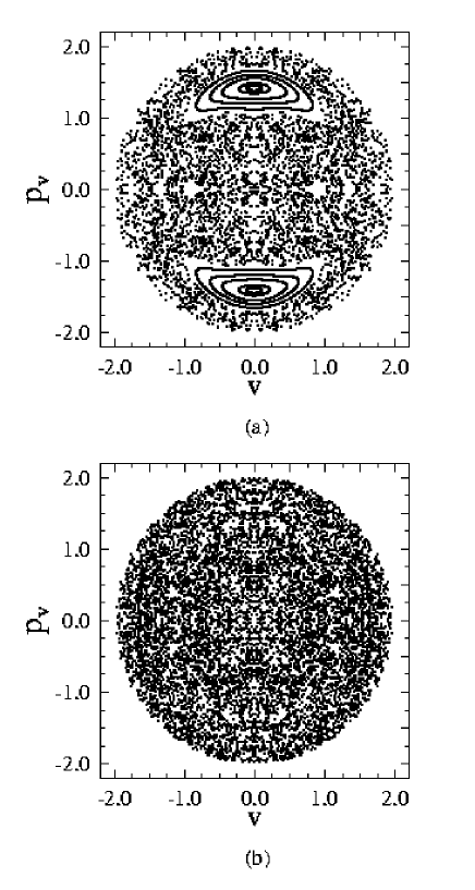
FIG. 1.: Poincaré surfaces of section at scaled energy $\tilde{E}=\tilde{H}(\epsilon=0)=-1/2$ and (a) $\omega_{L}n_{0}^{3}=3$, (b) $\omega_{L}n_{0}^{3}=9.2$. The sections are on the $v-p_{v}$ planes defined by $u=0$, $p_{u}>0$. In (a) five regular and one chaotic trajectories are shown, in (b) only one chaotic trajectory is followed. The centre of the atom corresponds to $v=0$.

FIG. 2.: Example of diffusive energy excitation $\langle(\Delta E)^{2}\rangle/E_{0}^{2}$ with the number of microwave periods $\tau$, for $\omega_{L}n_{0}^{3}=3$, $\epsilon_{0}=0.005$ and $\omega_{0}=0.1$. The straight line fit allows to determine $D_{B}/D_{0}=0.062$ via the relation $<(\Delta E)^{2}>=(2\pi D_{B}/\omega)\tau$.

FIG. 3.: Dependence of the scaled diffusion rate $D_{B}/D_{0}$ on the scaled frequency $\omega_{0}$ for $\epsilon_{0}=0.005$, $\omega_{L}n_{0}^{3}=3$ (full circles) and $\omega_{L}n_{0}^{3}=9.2$ (open circles). The straight lines show the theoretical dependence for $\omega_{0}\ll 1$ (Eq.(24)) and $\omega_{0}\gg 1$ (Eq.(25)), with $\chi_{1}=25$, $\chi_{2}=0.8$ ($\omega_{L}n_{0}^{3}=3$), $\chi_{1}=16$, $\chi_{2}=1.6$ ($\omega_{L}n_{0}^{3}=9.2$). Ensembles from $200$ to $1000$ trajectories, initially distributed microcanonically on the energy shell, have been used. The insert shows $D_{B}/D_{0}$ as a function of the scaled Larmor frequency $\omega_{L}n_{0}^{3}$, for $\epsilon_{0}=0.005$ and $\omega_{0}=0.1$.

FIG. 4.: Classical (full circles) and quantum (open triangles) scaled diffusion rates, for $\omega_{L}n_{0}^{3}=3$. In the quantum case $n_{0}=60$, $0.01\leq\epsilon_{0}\leq 0.04$. The insert shows an example of diffusive energy excitation in the quantum case, for $\omega_{L}n_{0}^{3}=3$, $\epsilon_{0}=0.02$, $\omega_{0}=0.1$; the straight line fit gives $D_{B}/D_{0}=0.055$.

FIG. 5.: Gamma ratio $\Gamma_{B}/\Gamma_{0}$ vs. scaled frequency $\omega_{0}$, for $\omega_{L}n_{0}^{3}=3$, $n_{0}=40$ (full line), $n_{0}=60$ (dotted line), $n_{0}=80$ (dashed line). The one–photon transition rate $\Gamma_{B}$ is evaluated according to Fermi’s Golden Rule (Eq.(30)), with the Dirac delta function substituted by a Lorentzian function, with spread $\tilde{\epsilon}=0.5/\rho_{B}$, where $\rho_{B}=0.34n_{0}^{4}$ is the density of states. Full circles show classical values of $D_{B}/D_{0}\omega_{0}^{2}$ at $\omega_{L}n_{0}^{3}=3$.

FIG. 6.: Scaled density of states $\rho_{B}/n^{4}$ as a function of $n$ for $\omega_{L}n_{0}^{3}=3$ (full circles) and $\omega_{L}n_{0}^{3}=9.2$ (open circles) at $n_{0}=60$. Solid and dashed lines refer to the quasiclassical computation (Eq.(33)). The insert gives quasiclassical scaled density of states vs. scaled Larmor frequency. The straight line shows the theoretical asymptotical dependence ($\rho_{B}/n_{0}^{4}=c/\omega_{L}n_{0}^{3}$, with $c=1.5$).

FIG. 7.: Probability distribution vs. number of absorbed photons $N_{\phi}$: quantum distribution $f_{\lambda}$ over the eigenbasis at $\epsilon=0$ (full curve); quantum probability in one–photon intervals $f_{N}$ (circles); classical probability in one–photon intervals (dotted line). The straight line shows the fit for the exponential localization. Parameter values: $n_{0}=50$, $\omega_{0}=1.3$, $\omega_{L}n_{0}^{3}=3$, $\epsilon_{0}=0.008$; scaled diffusion rate $D_{B}/D_{0}=0.53$, theoretical localization length estimate (Eq.(31)) $\ell_{B}=2.8$; (a) $80\leq\tau\leq 100$, $\ell_{BN}=2.1$; (b) $180\leq\tau\leq 200$, $\ell_{BN}=2.4$. In the classical simulation $1000$ trajectories are included in the microcanonical ensemble.

FIG. 8.: Same as in Fig.7, with $n_{0}=50$, $\omega_{0}=0.2$, $\omega_{L}n_{0}^{3}=3$, $\epsilon_{0}=0.007$, $D_{B}/D_{0}=0.090$, $\ell_{B}=15.4$, (a) $80\leq\tau\leq 100$, $\ell_{BN}=18$; (b) $180\leq\tau\leq 200$, $\ell_{BN}=18.8$ (in both cases the fit is limited to $0\leq N_{\phi}\leq 60$). The classical ensemble consists of $1000$ trajectories.

FIG. 9.: Dependence of the quantum (full curve) and classical (dotted curve) photon number square variance $<(\Delta N_{\phi})^{2}>$ on the number of microwave periods $\tau$ for $n_{0}=60$, $\omega_{0}=0.1$, $\epsilon_{0}=0.005$, $\omega_{L}n_{0}^{3}=3$. The classical ensemble consists of $5000$ trajectories.

FIG. 10.: The numerically computed localization length $\ell_{BN}$ vs. the theoretical estimate $\ell_{B}$ (Eq.(31)) for $\epsilon_{0}=0.005$ (full circles) and $\epsilon_{0}=0.01$ (open circles). Data are for $\omega_{L}n_{0}^{3}=3$ or $9.2$, $n_{0}=60$, $0.05\leq\omega_{0}\leq 3$. The straight line corresponds to $\ell_{BN}=\ell_{B}$.

FIG. 11.: Chaotic enhancement of microwave excitation. Same as in Fig.7, with $n_{0}=66$, $\omega_{0}=2.5$, $\omega_{L}n_{0}^{3}=3$, $\epsilon_{0}=0.04>\epsilon_{q}=0.016$, $D_{B}/D_{0}=0.97$, $40\leq\tau\leq 50$. Full triangles, linked by a dashed line, give quantum probability in one–photon intervals at the same parameter values but without magnetic field, $290\leq\tau\leq 300$ and with initial value of the orbital momentum quantum number $l_{0}=5$. In the latter case, $\epsilon_{c}=0.015<\epsilon_{0}<\epsilon_{q0}=0.14$, theoretical $\ell_{\phi_{\omega}}=1.1$, numerical $\ell_{\phi_{\omega}}=1.7$.

FIG. 12.: Quantum (full curve) and classical (dotted curve) square variance of the photon number vs. the number of microwave periods for the case of Fig.11. Above and upper scale: $\omega_{L}n_{0}^{3}=3$, below and lower scale: $\omega_{L}n_{0}^{3}=0$. The case $\omega_{L}=0$ is followed for a longer interaction time than for $\omega_{L}n_{0}^{3}=3$ to emphasize dynamical localization effects.

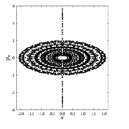
FIG. 13.: Poincaré surface of section for Na at $\epsilon_{s0}=0.02$, $n_{0}=60$. The $v-p_{v}$ plane of section is defined by $u=0$, $p_{u}>0$. The section is constructed following only one trajectory. Core potential parameters are $\alpha_{1}=2.48$, $\alpha_{2}=0.54$, $\alpha_{3}=1.43$.

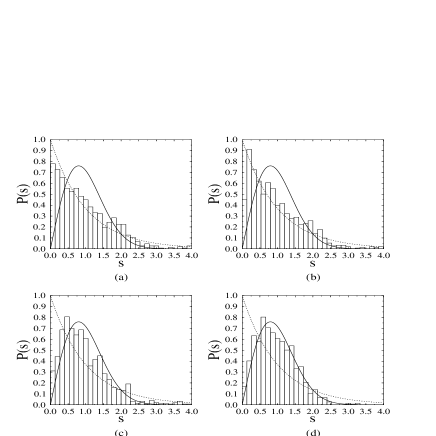
FIG. 14.: Level spacing statistics $P(s)$ for alkali atoms in a static electric field, with $\epsilon_{s0}=0.02$, $n_{0}=60$, $55\leq n\leq 72$, for (a) H, (b) Li, (c) Na and (d) Rb. The dotted line shows the Poisson distribution, the solid line is the Wigner–Dyson distribution (Eq.(47)).

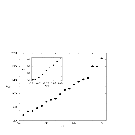
FIG. 15.: Inverse participation ratio $\xi$ (Eq.(48)) for Rb, at $\epsilon_{s0}=0.02$ and $n_{0}=60$, as a function of $n$. The insert shows the dependence of $\xi$ on $\epsilon_{s0}$, for $n_{0}=60$.

FIG. 16.: Dependence of the scaled classical diffusion rate $D_{c}/D_{0}$ on the scaled frequency $\omega_{0}$ for alkali Rydberg atoms in a static electric field, at $\epsilon_{0}=0.005$, $\epsilon_{s0}=0.02$, $n_{0}=60$ for Rb (circles), Na (triangles) and Li (squares). The straight lines show the theoretical dependence for $\omega_{0}\ll 1$ and $\omega_{0}\gg 1$, with $\chi_{1}=140$, $\chi_{2}=0.3$. Ensembles from $200$ to $1000$ trajectories, initially distributed microcanonically on the energy shell, have been used. Core potential parameters for Na as in Fig.13, for Rb $\alpha_{1}=3.10$, $\alpha_{2}=1.56$, $\alpha_{3}=0.76$ and for Li $\alpha_{1}=2.84$, $\alpha_{2}=4.05$, $\alpha_{3}=4.26$. The insert shows, for Rb at $\omega_{0}=0.1$, $n_{0}=60$, the dependence of $D_{c}/D_{0}$ on $\epsilon_{s0}$ for $\epsilon_{0}=0.0005$ (diamonds) and the more flat behavior for $\epsilon_{0}=0.005$ (circles).

FIG. 17.: Dependence of $\langle(\Delta E)^{2}\rangle/E_{0}^{2}$ on the number of microwave periods $\tau$, for $n_{0}=60$, $\epsilon_{s0}=0.02$, $\epsilon_{0}=0.005$, $\omega_{0}=1$. The straight line fits give $D_{c}/D_{0}=1.4$ (for $0\leq\tau\leq 10$) and $D_{c}/D_{0}=0.17$ (for $10\leq\tau\leq 70$).

FIG. 18.: Quantum scaled diffusion rate $D_{q}/D_{0}$ vs. frequency $\omega_{0}$ for Rb (full circles), Na (full triangles) and Li (full squares) at $\epsilon_{s0}=0.02$, $n_{0}=60$, $0.005\leq\epsilon_{0}\leq 0.03$. Open circles show the classical scaled diffusion rate $D_{c}/D_{0}$ for Rb, with parameters $\alpha_{i}$ as in Fig.16.

FIG. 19.: Probability distribution vs. number of absorbed photons $N_{\phi}$: quantum distribution $f_{\lambda}$ over the Stark eigenstates (full curve), quantum probability in one–photon intervals $f_{N}$ (circles) and classical probability in one–photon intervals (dotted line) for Rb at $n_{0}=60$, $\epsilon_{s0}=0.02$, $\omega_{0}=0.08$, $\epsilon_{0}=0.005$, $180\leq\tau\leq 200$. Here $D_{q}/D_{0}=0.0047$ and the theoretical localization length (Eq.(49)) is $\ell_{q}=13$. The straight line shows the fit for the exponential localization, with $\ell_{qN}=13$. Diamonds give $f_{N}$ (shifted down by $10^{3}$) for Rb under the same conditions, except for $\epsilon_{0}=0.002$, $\ell_{q}=2.1$. The straight line shows the fit for $0\leq N_{\phi}\leq 20$ ($\ell_{qN}=3.7$), whereas the fit for $N_{\phi}\geq 50$ gives $\ell_{qN}=28$. Classical data are obtained with $\alpha_{i}$ parameters as in Fig.16.

FIG. 20.: The numerically computed localization length $\ell_{qN}$ vs. the theoretical estimate $\ell_{q}$ (Eq.(49)) for Rb (full circles) and Na (full triangles) at $n_{0}=60$, $\epsilon_{s0}=0.02$, $\epsilon_{0}=0.005$, $0.02\leq\omega_{0}\leq 0.5$. The straight line corresponds to $\ell_{qN}=\ell_{q}$.

FIG. 21.: Same as in Fig.19 but above the delocalization threshold $\epsilon_{q}$ (Eq.(50)), for Rb at $n_{0}=60$, $\epsilon_{s0}=0.02$, $\omega_{0}=0.08$, $D_{q}/D_{0}=0.0047$, $\epsilon_{0}=0.03>\epsilon_{q}=0.027$, $40\leq\tau\leq 50$.

FIG. 22.: Same as in Fig.19, for the conditions of Fig.2d in [21], for Na at $n_{0}=28$, $\epsilon_{s0}=0.024$, $\omega_{0}=0.027$, $\epsilon_{0}=0.002$, $180\leq\tau\leq 200$, $D_{q}/D_{0}=0.0027$, $\ell_{q}=1.1$, $\ell_{qN}=4$ (straight line) for $f_{N}>10^{-5}$ and $\ell_{qN}=25$ for $f_{N}<10^{-5}$.

FIG. 23.: Probability distribution over the spherical hydrogenic basis for the case of Fig.22. Time evolution is followed under the same static and microwave field conditions, starting from a hydrogenic eigenstate with $n_{0}=28$ and initial value of the orbital momentum quantum number $l_{0}=2$, with absorption parameters (Eq.(51)) given by $\gamma_{n}=1/2\pi n_{s}^{3}$ for $\epsilon_{s}n^{4}>0.13$ ($n>n_{s}=42$). The insert shows that ionization probability depends on time in a nearly linear way (for the interaction time here considered, $\tau\leq 200$), with ionization rate (per microwave period) $\Gamma=2.5\times 10^{-4}$.

REFERENCES

- [1] Present address: CEA, Service de Physique de l’Etat Condensé, Centre d’Etudes de Saclay, F–91191 Gif–sur–Yvette, France
- [2] Also Budker Institute of Nuclear Physics, 630090 Novosibirsk, Russia
- [3] J.E. Bayfield and P.M. Koch Phys. Rev. Lett. 33, 258 (1974).
- [4] N.B. Delone, V.P. Krainov, and D.L. Shepelyansky, Sov. Phys. Usp. 26, 551 (1983) [Usp. Fiz. Nauk 140, 355 (1983)].
- [5] G. Casati, B. Chirikov, D.L. Shepelyansky, and I. Guarneri, Phys. Rep. 154, 77 (1987).
- [6] R. Blümel and U. Smilansky Z. Phys. D 6, 83 (1987).
- [7] G. Casati, I. Guarneri, and D.L. Shepelyansky, IEEE Journal of Quantum Electronics 24, 1420 (1988).
- [8] R.V. Jensen, S.M. Susskind, and M.M. Sanders, Phys. Rep. 201, 1 (1991).
- [9] P.M. Koch and K.A.H.van Leeuwen, Phys. Rep. 255, 289 (1995).
- [10] D.L. Shepelyansky, Physica D 28, 103 (1987).
- [11] A. Buchleitner and D. Delande, Phys. Rev. Lett. 70, 33 (1993); J. Opt. Soc. Am. B 12, 505 (1995).
- [12] J. Zakrzewski, R. Grebarowski, and D. Delande Phys. Rev. A 54, 691 (1996).
- [13] E.J. Galvez, B.E. Sauer, L. Moorman, P.M. Koch, and D. Richards, Phys. Rev. Lett. 61, 2011 (1988).
- [14] J.E. Bayfield, G. Casati, I. Guarneri, and D.W. Sokol, Phys. Rev. Lett. 63, 364 (1989).
- [15] M. Arndt, A. Buchleitner, R.N. Mantegna, and H. Walther, Phys. Rev. Lett. 67, 2436 (1991).
- [16] G. Casati, I. Guarneri, and D.L. Shepelyansky, Physica A 163, 205 (1990).
- [17] F.L. Moore, J.C. Robinson, C.F. Bharucha, P.E. Williams, and M.G. Raizen, Phys. Rev. Lett. 73, 2974 (1994); J.C. Robinson, C.F. Bharucha, F.L. Moore, R. Jahnke, G.A. Georgakis, Q. Niu, M.G. Raizen, and B. Sundaram, Phys. Rev. Lett. 74, 3963 (1995); F.L. Moore, J.C. Robinson, C.F. Bharucha, B. Sundaram, and M.G. Raizen, Phys. Rev. Lett. 75, 4598 (1995); J.C. Robinson, C.F. Bharucha, K.W. Madison, F.L. Moore, B. Sundaram, S.R. Wilkinson, and M.G. Raizen, Phys. Rev. Lett. 76, 3304 (1996).
- [18] D. Delande in Chaos and Quantum Physics edited by M.–J. Giannoni, A. Voros, and J. Zinn–Justin (North–Holland, Amsterdam, 1991), p. 665.
- [19] H. Friedrich and D. Wingten, Phys. Rep. 183, 37 (1989).
- [20] H. Hasegawa, M. Robnik, and G. Wunner, Progr. Theor. Phys. Suppl. 98, 198 (1989).
- [21] M. Courtney, N. Spellmeyer, H. Jiao, and D. Kleppner, Phys. Rev. A 51, 3604 (1995).
- [22] P. Pillet, H.B. van den Heuvell, W.W. Smith, R. Kachru, N.H. Tran, and T.F. Gallagher, Phys. Rev. A 30, 280 (1984); T.F. Gallagher, C.R. Mahon, P. Pillet, P. Fu, and J.B. Newman, Phys. Rev. A 39, 4545 (1989).
- [23] C.Y. Lee, J.M. Hettema, T.F. Gallagher, and C.W.S. Conover, Phys. Rev. A 46, 7048 (1992).
- [24] N. Spellmeyer, D. Kleppner, M.R. Haggerty, V. Kondratovich, J.B. Delos, and J. Gao, Phys. Rev. Lett. 79, 1650 (1997).
- [25] O.P. Sushkov and V.V. Flambaum, Sov. Phys. Usp. 25, 1 (1982) [Usp. Fiz. Nauk 136, 3 (1982)].
- [26] D.L. Shepelyansky, Phys. Rev. Lett. 73, 2607 (1994).
- [27] F. Benvenuto, G. Casati, and D.L. Shepelyansky, Phys. Rev. A 55, 1732 (1997).
- [28] G. Benenti, G. Casati, and D.L. Shepelyansky, Phys. Rev. A 56, 3297 (1997).
- [29] G. Benenti, G. Casati, and D.L. Shepelyansky, Phys. Rev. A 57, 1987 (1998).
- [30] D.C. Sorensen, SIAM J. Mat. Anal. Appl. 13, 357 (1992).
- [31] P.A. Dando, T.S. Monteiro, W. Jans, and W. Schweizer, Progr. Theor. Phys. Suppl. 116, 403 (1994).
- [32] B. Hüpper, J. Main, and G. Wunner, Phys. Rev. A 53, 744 (1996).
- [33] L.D. Landau and E.M. Lifshitz, Quantum Mechanics (Pergamon, New York, 1977).
- [34] C.–J. Lorenzen and K. Niemax, Phys. Scr. 27, 300 (1983); T.P. Hezel, C.E. Burkhardt, M. Ciocca, L.–W. He, and J.J. Leventhal, Am. J. Phys. 60, 329 (1992).
- [35] O. Bohigas in Chaos and Quantum Physics edited by M.–J. Giannoni, A. Voros, and J. Zinn–Justin (North–Holland, Amsterdam, 1991), p. 89.
- [36] R. Blümel, A. Buchleitner, R. Graham, L. Sirko, U. Smilansky, and H. Walther, Phys. Rev A 44, 4521 (1991).
- [37] I.M. Beterov, A.O. Vyrodov, I.I. Ryabtsev, and N.V. Fateev, Sov. Phys. JETP 74, 616 (1992) [Zh. Eksp. Teor. Fiz. 101, 1154 (1992)]; A.V. Bezverbnyǐ, I.M. Beterov, A.M. Tumaĭkin, and I.I. Ryabtsev, JETP 84, 437 (1997) [Zh. Eksp. Teor. Fiz. 111, 796 (1997)].
- [38] G. Casati, I. Guarneri, M. Leschanz, D.L. Shepelyansky, and C. Sinha, Phys. Lett. A 154, 19 (1991); F. Borgonovi and D.L. Shepelyansky, Phys. Rev. E 51 (1995) 1026.