Dynamical partitions of space in any dimension

Tomaso Aste

AAS, Sal. Spianata Castelletto 16, 16124 Genova Italy, and

LDFC, Institut de Physique,

Université Louis Pasteur, 67084 Strasbourg France

e-mail: tomaso@ldfc.u-strasbg.fr

Abstract

Topologically stable cellular partitions of $D$ dimensional spaces are studied. A complete statistical description of the average structural properties of such partition is given in term of a sequence of ${D\over 2}-1$ (or ${D-1\over 2}$) variables for $D$ even (or odd). These variables are the average coordination numbers of the $2k$-dimensional polytopes ($2k<D$) which make the cellular structure. A procedure to built $D$ dimensional space partitions trough cell-division and cell-coalescence transformations is presented. Classes of structures which are invariant under these transformations are found and the average properties of such structures are illustrated. Homogeneous partitions are constructed and compared with the known structures obtained by Voronoï partitions and sphere packings in high dimensions.

1 Introduction

We study topologically-stable division of any dimensional space by cells. Such systems have minimal incidence numbers. Configurations with higher incidence numbers are topologically unstable because they can be splited into configurations with the minimal incidence numbers by infinitesimal local transformations. In the literature these cellular partitions are known as “froths” since in two and three dimensions ($2D$ and $3D$) the soap froth is the archetype of such structures. A $2D$ froth is a space-filling cellular partition made of irregular polygons where on each vertex are incident three polygons. A $3D$ froth is a polyhedral partition of space where on each vertex are incident 4 polyhedra. In general, a $D$-dimensional froth is a partition of space in irregular polytopes, where on each vertex $D+1$ polytopes are incident. Cellular structures with minimal incidence numbers always appear when the space is filled by cells without following any special symmetry. Therefore, froths are the typical structures of any disordered partition of the space in cells.

A broad class of disordered natural and artificial cellular systems have the topological structure of froths [1, 2, 3]. Examples in two dimensions are magnetic domains in garnets films, Bérnard-Marangoni cells in thermal convections, biological tissues, cuts of polycrystalline metals and ceramics, emulsions, the subdivision of territory in administrative regions or in national states, geological structures and $2D$ soap froth (which is obtained by squeezing the soap foam between two plates) [4, 5, 6]. In three dimensions, examples are biological cells, polycrystalline metals and ceramics, foams [4, 7, 8]. Moreover, the structure of any packing (of hard spheres or atoms, for example) is the dual of a cellular system (which can be generated, for instance, by using the Voronoï construction [9] around the centers of the packed elements). In general, cellular systems generated by packings elements without the use of any specific symmetry have structures which are topologically froths. It follows that, among the examples of $3D$ froths one can include amorphous metals, glasses and some crystalline structures such as the tetrahedrally closed-packed phases (t.c.p.) [10, 11].

Froths in spaces with dimensionality higher than 3 are relevant in information theory and signal processing [12, 13]. Indeed, an information can be associated with a point in an $N$-dimensional space. To transmit and recover the information in presence of noise one must put the points in the $N$-dimensional space, separated by a certain distance which must be larger than the additional noise. Therefore to each point (information) is associated a finite volume and the entire space is subdivided in cells each one containing one encoded information [12]. The energy necessary to transmit an information is proportional to the distance of the representing point respect to the origin. An efficient coding, which minimizes the energy, organizes the volumes associated with the different information in the closest possible packing of similar cells around the origin [13].

Dense packings of equal cells in high dimensions have also applications in the study of analogue-digital converters. In this case, the space of the continuous analogical variables is quantized in a system of cells and the volume inside each cell is associated with one digital information. The quantization error is associated with the extension of the interface between the cells and with the distance between the center of a cell and its vertices [13].

High dimensional partition of space has also application in neural networks and complex system dynamics [14, 15, 16, 17, 18]. Some relevant properties (such as the storage capacity in neural network and the slow aging dynamics in glasses) are associated with the subdivision of the phase-space in basin of attraction around the stored information or the minima of the energy.

Two and four dimensional froths (and their duals: triangulations and simplicial decompositions) have relevance in quantum gravity [19, 20, 21, 22, 23, 24]. Here the continuous space is divided into cells and the functional integration over all equivalence classes of metrics is replaced with a summation over all the triangulations of the given manifold.

Despite the broad variety of system which are topologically froths and the large amount of studies devoted to them in the literature, very little is known about the structure of froths in dimensions larger than $D=3$. Froths are disordered cellular structures where the cells are highly correlated. These correlations essentially come from the space-filling condition which locally constraints the cells to pack without leaving any empty space, and globally constraints the froth to tile a manifold with a given curvature. In this paper we study how these local and global conditions determinate the average topological properties of the froth structure and we construct froths in any dimension by cell-division and coalescence transformations. The aim of the present paper is to investigate the average structural properties of classes of homogeneous partitions of high dimensional Euclidean spaces and to give analytical instruments and methodologys for the the investigation of the topological structure of froths in spaces of arbitrary dimensions and curvature.

The plan of the paper is the following: In Section 2, the hierarchical organization of topologically stable divisions of space in cells is studied; In Section 3, we discuss a way to generate or modify $D$-dimensional froths by cell-division and cell-coalescence transformations; In Section 4, the fixed points of such transformations are studied and the properties of the associated structures are illustrated; The construction of homogeneous partitions and the comparison of their properties with known structures, is done in Section 5.

2 Hierarchy in the cellular structure

A froth in an arbitrary dimension $D$ is a cellular structure where the incidence numbers (i.e. the average number of elements which are incident on a given lower-dimensional element) are fixed by the stability condition at the minimal value. The cells of a froth in dimension $D$ are $D$-dimensional irregular polytopes packed together to fill space. The boundaries of these cells are made with $(D-1)$-dimensional polytopes which are bounded by $(D-2)$-dimensional polytopes and so on up to the zero-dimensional elements which are the vertices. For example, a three dimensional froths is made with $3D$ polyhedra (the cells) which are bounded by $2D$ polygons (the faces) which are bounded by $1D$ elements (the edges) finally bounded by $0D$ elements (the vertices). A characterization of this $D$-dimensional structure can be given in term of the numbers of $D$-dimensional polytopes which are making the froth, in term of the average numbers of $(D-1)$-dimensional polytopes making the boundary of a given cell and so on counting the number of polytopes making the boundary of the boundary, etc.

The boundary of any $k$-dimensional polytope of the froth is also a froth in a $(k-1)$-dimensional elliptic space. The $D$–dimensional froth is therefore a graded topological set: it contains $D$–polytopes, the cells, which are tiling a space which can be Euclidean, elliptic or hyperbolic. The boundary of each cell is an elliptic $D-1$ surface which is tiled by a $(D-1)$-dimensional froth, whose cells are $(D-1)$–polytopes which are the interfaces bounding the original cell and separating it from its topological neighbours. Each interface of the $(D-1)$–froth is an elliptic $(D-2)$–froth of $(D-2)$–polytopes, which are separating the cells from their neighbours. The graded topological set terminates with edges (segments or convex 1–polytopes), bounded by 2 vertices (or 0–polytopes).

Let denote with $C_{k}$ the number of $k$-dimensional cells in the froth ( $C_{0}$ number of vertices, $C_{1}$ number of edges, $C_{2}$ number of faces, $C_{3}$ number of polyhedra … $C_{D}$ number of $D$-dimensional cells.). Let denote with $\langle n_{i,j}\rangle$ (for $i\leq j$) the average number of $i$-dimensional cells which are surrounding and making the boundary of a $j$ dimensional cell ($\langle n_{0,1}\rangle=2$ number of vertices surrounding an edge, $\langle n_{1,2}\rangle$ number of edges per faces, etc.).

The average froth structure is characterized by the numbers of polytopes $C_{i}$ and by the valences $\langle n_{i,j}\rangle$ (with $0\leq i<j\leq D$), which are therefore the variables of the problem. The total number of these variables is ${1\over 2}(D+1)(D+2)$, but they are related by the Euler equations and constrained by the stability condition. In particular, the numbers of elements in the froth $C_{i}$ are related through the Euler relation:

$$\sum_{i=0}^{D}(-1)^{i}C_{i}=\chi_{D}\;\;\;,$$ (1)

where $\chi_{D}$ is the Euler–Poincaré characteristic which is associated with the space curvature. For $D$ even, opposite signs of $\chi_{D}$ correspond to spaces with opposite curvature: $\chi_{D}>0$ corresponds to an elliptic $D$–dimensional space and $\chi_{D}<0$ corresponds to an hyperbolic space. On the other hand, for $D$ odd, this relation between the sign of $\chi_{D}$ and the space curvature does not holds anymore.

An Euler relation is also satisfied for each froth of the graded topological set. That gives a set of relations for the quantities $\langle n_{i,j}\rangle$

$$\sum_{i=0}^{J-1}(-1)^{i}\langle n_{i,J}\rangle=1-(-1)^{J}\;\;\;\;\mbox{(with $J=1,2,...,D$). }$$ (2)

Here the factor $1-(-1)^{J}=\chi_{J-1}^{(elliptic)}$ is the Euler–Poincaré characteristic for the surface of a $J$-dimensional sphere (which is a $(J-1)$-dimensional elliptic space).

The numbers $C_{i}$ and the averages $\langle n_{i,j}\rangle$ are related by the stability condition

$$\left(\begin{array}[]{cc}{D+1-i}\\ {j-i}\end{array}\right)C_{i}=\langle n_{i,j}\rangle C_{j}\;\;\;\;\mbox{(with $i\leq j\leq D$),}$$ (3)

where $n_{i,i}=1$. The binomial coefficient in the left-hand side of Eq.(3) is an incidence number (number of $j$-dimensional polytopes incident on an $i$-dimensional polytope) which is fixed at the minimum value by the stability condition (there are $(D+1)$ edges and $\big{(}^{D+1}_{\;\;2}\big{)}$ faces incident on each vertex, $D$ faces incident on each edge, etc.).

By contrast, the coordination numbers $\langle n_{i,j}\rangle$ with $i<j$ are variables (except for $n_{0,1}$: every edge is bounded by two vertices and therefore $n_{0,1}=2$). These variables are not all independent and their range of variability is severely restricted by relations (1), (2) and (3) (for example, in a $2D$ infinite Euclidean froth we have $\langle n_{1,2}\rangle=\langle n_{0,2}\rangle=6$ as consequence of the Euler relation).

One can show that [25] a complete topological characterization of the average structure of a $D$–froth is given by a set of ${D\over 2}-1$ (or ${D-1\over 2}$) for $D$ even (or odd), independent variables: the even “valences” $X_{2l}=\langle n_{2l-1,2l}\rangle$ with $2l<D$. These valences are the average coordination numbers (average number of neighbours) of the $2l$–dimensional polytopes in the froth. These are free variables. On the contrary, the coordination numbers for the odd dimensional polytopes (the odd valences) are given in terms of the even valences by the relations

$$\frac{X_{1}X_{2}\cdots X_{J}}{(J)!}-\frac{X_{2}\cdots X_{J}}{(J-1)!}+\cdots-(-1)^{J}\frac{X_{J-1}X_{J}}{2}+(-1)^{J}X_{J}=1-(-1)^{J}\;\;\;\mbox{(for $J=1,2,....D$)}.$$ (4)

(Which is obtained from Eq.(2) associated with Eq.(3) and by using the definition $X_{k}=\langle n_{k-1,k}\rangle$.) For $J=2l+1$ odd, the left hand term in Eq.(4) is equal to 2 and Eq.(4) fixes the value of the odd valence $X_{2l+1}$ in terms of the even ones. When $J=2l$ even, the left hand term is zero and therefore the even valences $X_{2l}$ are free variables.

In $k$ dimensions the polytope with minimal coordination number is a simplex with $k+1$ neighbours. Therefore, the valences must stay into the range $k+1\leq X_{k}<\infty$. The average structure of a $D$-dimensional froth is characterized by a sequence of even free valences $\{X_{2},X_{4},X_{6}.....\}$. For any given sequence of even valences $\{X_{2l}\}$ the odd ones can be calculated by using equations (4). But only sequences which generate odd valences with $X_{2l+1}\geq 2l+2$ are admissible. This condition strongly constraint the accessible values of the even valences.

The Euler’s formula (1), associated with Eq.(4) and Eq.(3), gives an additional relation between valences

$$\Bigg{(}\frac{X_{1}X_{2}\cdots X_{D}}{(D+1)!}-\frac{X_{2}\cdots X_{D}}{(D)!}+\cdots-(-1)^{D}\frac{X_{D}}{2}+(-1)^{D}\Bigg{)}C_{D}=\chi_{D}\;.$$ (5)

In even dimensional spaces, the sign of the Euler–Poincaré characteristic $\chi_{D}$ is associated with the space-curvature. The sign of the term inside the brackets in the left-hand side of Eq.(5) is the same of $\chi_{D}$ (because $C_{D}>0$). Therefore, any two regions of the valences’ space which have different signs of the bracket term (i.e. of the $\chi_{D}$) correspond to two froths on manifolds of opposite Gaussian curvature. For example, in the $2D$ case (where the average structure of the froths is described by the parameter $X_{2}$) equation (5) gives

$$(6-X_{2}){C_{2}\over 2}=\chi_{2}\;\;\;,$$ (6)

which indicates that $2D$ froths with $X_{2}<6$ are tiling elliptic surfaces, whereas froths with $X_{2}>6$ are tiling hyperbolic surfaces (see fig.(1a)). In four dimensions Eq.(5) gives

$$X_{4}=\Big{(}1-{\displaystyle\chi_{4}\over C_{4}}\Big{)}5{\displaystyle 6-X_{2}\over 5-X_{2}}\;\;,$$ (7)

(where we used Eq.(4) to express $X_{3}$ as a function of $X_{2}$). Equation (7) indicates that the region in the parameter space $\{X_{2},X_{4}\}$ below the line $X_{4}=5{6-X_{2}\over 5-X_{2}}$ is associated with $4D$ froths which are tiling elliptic manifolds ($\chi_{4}>0$), whereas the region above this line correspond to froths tiling hyperbolic manifolds ($\chi_{4}<0$) (see fig.(1b)).

Note that Eq.(4) is a constraint on the sequence $\{X_{2l}\}$ given by local conditions (it concerns the average properties of a $2l+1$ dimensional polytope in terms of the properties of the lower dimensional elements that are making it). Whereas, Eq.(5) is a constraint on $\{X_{2l}\}$ given by the global curvature of the manifold that the froth is tiling.

Note also that relation (7) has a singularity in $X_{2}=5$. This is associated with the existence of polytope $\{5,3,..\}$ (Schlälfly symbols [26]) up to $D=4$ only, as explained in Appendix A.

3 Cell-division and cell-coalescence transformations

In this section we build $D$-dimensional froths by using the cell-division transformation and its inverse (the cell-coalescence). This is a local transformation that changes the structure of the froth but leave unchanged the global topological properties (the curvature of the manifold tiled by the froth or -equivalently- the parameter $\chi_{D}$). By using cell division and coalescence it is therefore possible to generate different froths which are tiling topologically identical manifolds.

In the literature analogous transformations have been studied for the dual problem of triangulations and simplicial decomposition. In particular, it is known that, given two different partitions of the $D$-dimensional space in $D$-simplices (where a 0-simplex is a point, 1-simplex an edge, 2-simplex a triangle, 3-simplex a tetrahedron, etc.), one can be transformed into the other by a finite sequence of two local transformations called “Alexander moves” [27]. The first move is the addition of a vertex inside a simplex dividing it in $D+1$ simplices with the same boundary of the original simplex. The second move correspond to add a vertex on an edge of a simplex and connecting it with the vertices of the incident simplexes. For the $2D$ case the two Alexander move are the insertion of a new vertex inside a triangle and the insertion of a new vertex on an existing edge. They are shown in fig.(2a) and (2b). In the dual froth these moves corresponds to a cell-division which inserts a triangle near to an existing vertex and to a cell-division which inserts a square near to an existing edge (fig.(2c) and (2d)). In $3D$, one can easily see, by following the same procedure illustrated for $2D$, that the two Alexander moves can be obtained in the dual space of the froth by applying cell-division transformations. In the general case, one can see that the first Alexander move can be always done in the dual froth by dividing a cell in the proximity of a vertex inserting in this way a new polytope with $D+1$ neighbours (a simplex). The second move can be done dividing a cell in the proximity of an existing $D-1$ dimensional interface between two cells. In this case, the kind of polytope inserted depends on the local configuration.

We have therefore shown that, the two Alexander moves are reduced in froths to two special kinds of cell-division transformations. Consequently, the entire set of all the possible froths tiling a given manifold can be generated by cell-division and its inverse (cell-coalescence) transformations.

Now we investigate how the average properties of the structure are modified by these transformations. First consider the cell-division transformation in the two dimensional case. The cut of a cell corresponds to insert in the system 1 additional face, 3 edges and 2 vertices. Therefore, one has the transformations $C_{2}\rightarrow C_{2}+1$, $C_{1}\rightarrow C_{1}+3$ and $C_{0}\rightarrow C_{0}+2$. One can verify that the Euler-Poincaré characteristic rests unchanged (indeed, $\chi_{D}=C_{0}-C_{1}+C_{2}$). On the contrary, the average coordination number (which is given by $X_{2}={2C_{1}\over C_{2}}$, see Eq.(3)) is modified

$$X_{2}^{\prime}=X_{2}\mp{\displaystyle 1\over C_{2}\pm 1}(X_{2}-6)\;\;\;\;,$$ (8)

with the upper sign corresponding to a cell-division transformation and the lower sign to its inverse (coalescence).

Now consider the $3D$ case. A cell-division corresponds to insert inside a cell a new face which can have, in general, $c_{1}$ edges and $c_{0}(=c_{1})$ vertices. This cut corresponds to the transformation $C_{3}\rightarrow C_{3}+1$, $C_{2}\rightarrow C_{2}+1+c_{1}$, $C_{1}\rightarrow C_{1}+c_{1}+c_{0}$ and $C_{0}\rightarrow C_{0}+c_{0}$. Equation (3) gives $X_{3}={2C_{2}\over C_{3}}$, and therefore we obtain that the average coordination number transforms as

$$X_{3}^{\prime}=X_{3}\mp{\displaystyle 1\over C_{3}\pm 1}\Bigl{(}X_{3}-2(c_{1}+1)\Bigr{)}\;.$$ (9)

In the $D$-dimensional case, the cut of a cell corresponds to introduce a $D-1$ dimensional interface which is, in general, made of $c_{0}$ vertices, $c_{1}$ edges, $c_{2}$ faces, $c_{3}$ 3-dimensional cells …. $c_{D-2}$ $(D-2)$-dimensional polytopes. Consequently, the division of a $D$-dimensional cell (or the coalescence between two cells) of the $D$-dimensional froth correspond to the transformation

$$C_{0} \rightarrow C_{0}\pm c_{0}$$

$$C_{1} \rightarrow C_{1}\pm c_{1}\pm c_{0}$$

$$C_{2} \rightarrow C_{2}\pm c_{2}\pm c_{1}$$

$$\vdots$$

$$C_{k} \rightarrow C_{k}\pm c_{k}\pm c_{k-1}$$

$$\vdots$$

$$C_{D-1} \rightarrow C_{D-1}\pm 1\pm c_{D-2}$$

$$C_{D} \rightarrow C_{D}\pm 1\;\;\;,$$ (10)

where the upper sign $(+)$ corresponds to a cell-division transformation and the lower sign $(-)$ to its inverse (coalescence). By substituting into Eq.(1) one can verify that the global curvature ($\chi_{D}$) is an invariant quantity under the transformation (10). Note that, expression (10) takes the canonical form $C_{k}\rightarrow C_{k}\pm c_{k}\pm c_{k-1}$ for all $k$ if one impose $c_{-1}=0$, $c_{D-1}=1$ and $c_{D}=0$.

From Eq.(3) one has the identity $X_{k}C_{k}=(D+2-k)C_{k-1}$ (where we used the definition $X_{k}=\langle n_{k-1,k}\rangle$). By substituting in this expression the transformation (10) we get

$$X^{\prime}_{k}=X_{k}\mp{\displaystyle 1\over C_{k}\pm c_{k}\pm c_{k-1}}\Big{(}X_{k}(c_{k}+c_{k-1})-(D+2-k)(c_{k-1}+c_{k-2})\Big{)}\;\;,$$ (11)

(upper sign, cell-division; lower sign, cell-coalescence).

We recall that through cell-division/coalescence transformations it is possible to generate the full class of froths tiling topologically identical manifolds. The modification of the average structural properties associated with these geometrical transformation are algebraically given by equation (11). By using this expression it is therefore possible to find the average topological properties of all the froths on a given manifold.

4 Fixed points

When cell-division or coalescence transformations are performed on a $2D$ froth with average coordination $X_{2}=X^{*}_{2}=6$, they leave the local average structural properties unchanged (i.e. $X^{\prime}_{2}=X_{2}=X^{*}_{2}=6$, see Eq.(8)). This is a fixed point in the transformation (10) and corresponds to $2D$ Euclidean froths. Moreover, one can see that the average structural properties of froths which are tiling elliptic surfaces (i.e. the one with $X_{2}<6$) are modified toward the Euclidean structure ($X_{2}<X^{\prime}_{2}<6$) by the application of the cell division transformation. Analogously hyperbolic froths ($X_{2}>6$) are also modified towards the Euclidean structure ($6<X^{\prime}_{2}<X_{2}$) (see fig.(1a)). (Note that the global curvature remain always unchanged. Indeed, $\chi_{D}$ is an invariant under the transformation (10)).

In the general case, one can immediately see that transformation (11) has the fixed point

$$X_{k}^{*}=(D+2-k){\displaystyle c_{k-1}+c_{k-2}\over c_{k}+c_{k-1}}\;\;\;,$$ (12)

which is the structure that is invariant under cell-division/coalescence transformations ($\{{X^{*}_{k}}^{\prime}\}=\{X^{*}_{k}\}$).

A froth is a graded set. Therefore the $D-1$ dimensional interface that have been introduced into the system to cut a cell is a $(D-2)$-dimensional elliptic froth with $c_{0}$ vertices, $c_{1}$ edges …. $c_{D-2}$ $(D-2)$-dimensional cells. All the relations written above, and in particular Eqs.(2) and (3), can be applied to this $(D-2)$-dimensional elliptic froth. One has, $c_{k}x_{k}=(D-k)c_{k-1}$ and $c_{k-1}x_{k-1}=(D+1-k)c_{k-2}$, with $x_{k}$ and $x_{k-1}$ the average coordination numbers of the $k$ and $(k-1)$-dimensional polytopes which are making the $(D-1)$-dimensional interface. By substituting into Eq.(12), one gets

$$X_{k}^{*}={\displaystyle(D+2-k)(D+1-k+x_{k-1})\over(D+1-k)(D-k+x_{k})}x_{k}\;\;\;.$$ (13)

The fixed point configuration is therefore determined by a set of variables $\{x_{k}\}$ with $k<D$ which are the average coordinations of the ($D-1$)-dimensional polytope that is inserted or removed during the cell division or coalescence transformation. For example, in $D=3$, relation (13) gives

$$X^{*}_{3}=2x_{2}+2$$ (14)

with $x_{2}$ the number of edges of the face that is inserted (or removed) to divide a cell (or make coalescence between two cells).

The minimum number of edges per cell is 3. Therefore from Eq.(14) follows that fixed point structures are possible only in the region of the parameter space with $X_{3}\geq 8$ (see fig.(1 a)). Any structure with $X_{3}<8$, is transformed towards the fixed point region ($X_{3}\geq 8$) by applying cell-division transformations.

In four dimensions Eq.(13) gives

$$X^{*}_{2} = {\displaystyle 20x_{2}\over 3(2+x_{2})}$$

$$X^{*}_{4} = 2(x_{3}+1)=2\Big{(}{\displaystyle 12\over 6-x_{2}}+1\Big{)}\;.$$ (15)

We can express the parameter $x_{2}$ in Eq.(15) in terms of $X^{*}_{2}$ obtaining $X^{*}_{4}=5{6-X^{*}_{2}\over 5-X^{*}_{2}}$, which is the condition on the even valences that identifies the Euclidean region in 4-dimensional froths (see Eq.(7)). The fixed point structures are Euclidean. Since $x_{3}\geq 4$, follows $X_{4}^{*}\geq 10$, which implies that structures generated by cell division can only access to a part of the Euclidean region in the phase-space.

We can in general prove that the fixed point $\{X^{*}_{k}\}$ given by Eq.(13), is the average structure of a $D$-dimensional froth which is tiling a manifold with $\chi_{D}=0$. Indeed, let substitute into Eq.(5) the fixed point configuration ($\{X^{*}_{k}\}$) and apply the cell division transformation. By definition the sequence $\{X^{*}_{k}\}$ doesn’t change, whereas the total number of cells increases of a unity ($C_{d}\rightarrow C_{D}+1$). To satisfy Eq.(5) before and after this transformation one must have $\chi_{D}=0$. Which prove the theorem.

By re-writing Eq.(11) in the form

$$X^{\prime}_{k}=X_{k}\mp{\displaystyle(c_{k}+c_{k-1})\over C_{k}\pm c_{k}\pm c_{k-1}}\Big{(}X_{k}-X^{*}_{k}\Big{)}\;\;,$$ (16)

it is easy to see that the fixed points are stable under cell division transformations (upper sign in Eq.(16)) which inserts identical polytopes as interface. Indeed, from Eq.(16), if $X_{k}>X^{*}_{k}$ then $X_{k}>X^{\prime}_{k}>X_{k}^{*}$ and vice versa.

In the space of the configuration { $X_{2},X_{4},...,X_{2l},...$ }, when $D$ even, the Euclidean region is a surface given by Eq.(5) (with $\chi_{D}=0$). The fixed point configurations are a subset of this surface. Froths outside the fixed point configuration are always transformed toward this subset by applying cell-division transformations. When $D$ odd, Eq.(5) is not a constraint and the fixed point are associated with a sub-volume of the whole accessible parameter space.

5 Construction of Euclidean froths

In this paragraph we study froths generated by cell-division transformations. We therefore study the class of structures $\{X^{*}_{k}\}$ given by Eqs.(11) and (13). The full class of these froths is obtained by varying in Eq.(13) the parameters $\{x_{k}\}$ in the allowed range (i.e. $k+1\leq x_{k}<\infty$, which satisfy the conditions (4) for $k$ odd and the relation (5) with $\chi_{D}<0$). Here, we study only some particular cases.

Let us first note that, from Eq.(13), the average number of neighbours of the fixed point structure is given in term of the coordination of the inserted interface ($x_{D-1}$) by

$$X^{*}_{D}=2x_{D-1}+2\;\;\;\;.$$ (17)

In two dimensions an edge is inserted or removed from a face. The “coordination” of an edge is its number of vertices: $x_{D-1}=x_{1}=2$. Therefore $X^{*}_{2}=6$, as should be in Euclidean space. In three dimensions a face is inserted in, or removed from a cell. The coordination of this face ($x_{2}$) is its number of edges and in principle it can be any number between 3 and $\infty$. But, a face with a large number of edges can be inserted only in a cell with a large number of neighbours and it can be removed only if it exists in the froth. Therefore, only some values of $x_{2}$ are admissible. One can easily see that a triangle ($x_{2}=3$) can always be inserted in the proximity of a vertex. Analogously, a square ($x_{2}=4$) can also be always inserted in the proximity of an edge. From (17) follows therefore that three dimensional Euclidean froths with $8\leq X^{*}_{3}\leq 10$ can always be generated. But, in general, it should be possible to insert faces with higher values of $x_{2}$. To have an estimation for the “typical” value for the number of edges of the inserted face let make a cut of the whole three dimensional froth with a plane. The result is a two dimensional Euclidean froth where each single face is the result of a cut on a three dimensional cell. This two dimensional froth is therefore a representative set of faces produced by random cuts of three dimensional cells. The average number of edges for this set of faces is $x_{2}=X^{*}_{2}=6$. Therefore, from (17), a “typical” froth generated by cell division is expected to have a fixed point coordination around $X^{*}_{3}=14$ [28]. Cells in biological tissues appear in various polyhedral shapes with a number of faces distributed in a narrow range around 14 [29]. A widely studied three dimensional froth made with identical cells is the “Kelvin froth”, its cells are space-filling truncated octahedra with $X_{3}=14$ [30, 31]. Coordinations between 15.53 and 14 are found in Voronoï partition of space [32], where the higher value corresponds to a Voronoï partition from random points [35] whereas the lower value corresponds to more compact and homogeneous packings . Smaller values in the range $13.333\leq X^{*}_{3}\leq 13.5$ characterize an interesting class of natural structures (Frank-Kasper phases [33]) which partitionate the ordinary space with cells with pentagonal and hexagonal faces only. Soap froth has typically $X_{3}\simeq 13.7$ [34].

In a $D$-dimensional froth a ($D-1$)-dimensional interface with coordination $x_{D-1}$ is inserted or removed by cell division or coalescence transformations. As pointed out above, simplexes with coordinations $x_{D-1}=D$ can always be inserted in the proximity of an existing vertex. This is the minimum possible value for $x_{D-1}$ and substituted into Eq.(17) sets the minimum value of the average number of neighbours in a $D$-dimensional Euclidean fixed point structure at the minimal coordination

$$X^{*}_{D}=2D+2\;\;\;.$$ (18)

The argument for the “typical” cut that we used in three dimensions can be directly extended to any dimension. Indeed, one of the properties of froths is that a cut with an hyper-plane of a $D$-dimensional froth generates a $D-1$-dimensional Euclidean froth. For instance, a cut of a four dimensional froth give a three dimensional Euclidean froth. We can assume, that this froth has the “typical” coordination $X^{*}_{3}=14$ found above. Inserting into Eq.(17) one gets $X^{*}_{4}=30$. The same arguments, extended to any dimension, give

$$X^{*}_{D}=2^{(D+1)}-2\;\;\;\;\;,$$ (19)

for the average number of neighbours per cell in the “typical” $D$-dimensional froth.

What makes Eq.(13) powerful is the fact that, not only the average number of neighbours, but all the average properties of the fixed point structures can be deduced in term of the properties of the inserted interface.

5.1 Minimally coordinated froths

Let first construct the Euclidean froth with minimum coordination numbers. It is the fixed point structure associated to a cell-division transformation which inserts interfaces with minimal coordinations. This interfaces are $D-1$ dimensional simplices inserted in the proximity of vertex. They have $x_{k}=k+1$ (for $k<D$). By substituting into Eq.(13) one obtains

$$X^{*}_{k}={\displaystyle D+2-k\over D+1-k}(k+1)\;\;\;.$$ (20)

(Note that $X^{*}_{D}=2D+2$, as discussed above.) This are the average structural properties of a froth which is tiling a manifold with $\chi_{D}=0$ which is homologue to the Euclidean space. It is the known Euclidean forth with minimal coordination numbers. Starting from any given $D$-dimensional froth one can always transform it into this minimally coordinated one by applying an infinite number of cell-divisions near existing vertices. The resulting structure is expected to have cells with very different topological properties. Indeed, for each cell-division transformation a new cell with $D+1$ neighbours is inserted and 1 neighbour is added to the $D+1$ cells around the inserted simplex, distributing therefore the coordinations inhomogeneously between cells.

5.2 Homogeneous partitions

A $D$-dimensional froth has $D+1$ edges incident on each vertex. In an ideal homogeneous partition of space these edges are equally separated in angle. That corresponds to an angle $\theta^{ideal}=\cos^{-1}(-1/D)$ between each couple of edges [25]. In a froth, edges must close in rings which are bounding two dimensional faces. It is easy to see that with the angle $\theta^{ideal}$, flat rings close with an average number of edges equal to:

$$X_{2}^{ideal}={2\pi\over\pi-\cos^{-1}\big{(}-{1\over D}\big{)}}\;\;\;.$$ (21)

This number is 6 in two dimension, 5.104 in three dimensions, 4.767 for $D=4$, 4.588 for $D=5$ and tends to 4 when $D\rightarrow\infty$. Note that $X^{ideal}_{2}$ is irrational for $D>2$. In the Euclidean space, the “ideal” structure cannot be obtained by any ordered lattice structure. This is an example of geometrical frustration. But disordered or non-periodic structures can approximate $X_{2}^{ideal}$ with arbitrary precision avoiding in this way the frustration.

The average number of edges per cell $X_{2}^{ideal}$ (Eq.(21)) is the only quantity, of the ideal structure, that can be calculated by using these geometrical arguments. All the other coordinations are unknown, but we can construct fixed point structures that approximate this ideal froth in the ring coordination $X_{2}$. For these structures we can calculate the whole set of coordinations, and therefore we can infer information about the coordinations of the ideal one.

We expect that structures that partitionate uniformly space must have $X_{2}\simeq X^{ideal}_{2}$. By cell division transformation it is possible to generate froths that approximate the ideal structures by inserting interfaces with $x_{2}$ close to the ideal value $X^{ideal}_{2}$.

For $D=3$, $X^{ideal}_{2}=5.104$ which corresponds to $X_{3}^{ideal}=13.392$. In $3D$ we can generate homogeneous partitions by inserting pentagons $x_{2}=5$ or hexagons $x_{2}=6$ obtaining (from Eq.(17)) $12\leq X^{*}_{3}\leq 14$, which is in the right range.

In general, since we are looking for homogeneity, it is logical to insert as interfaces regular polytopes with $x_{2}$ close to the ideal value $X^{ideal}_{2}$. These polytopes can only be hyper-cubes {4,3…} (which have $x_{2}=4$) and the polytope {5,3…} (with $x_{2}=5$), but this second polytope exists only up to $D=4$ ([26] and App. A).

(a) Cell-division operations which inserts the polytope {5,3…} can therefore generate Euclidean fixed point structures up to $D=5$. In $D=3$ this corresponds to cell-divisions which insert pentagonal faces, that generates a fixed point structure with $X^{*}_{2}=5$ and $X_{3}^{*}=12$. In four dimensions, the fixed point structure obtained by inserting dodecahedra ({5,3}, $x_{2}=5$, $x_{3}=12$) has $X^{*}_{2}=100/21=4.7619...$ value that is very close to the ideal one. The four dimensional cells of this froth have $X^{*}_{4}=26$ neighbours in average. For $D=5$, by dividing cells with the polytope {5,3,3 } ($x_{2}=5$, $x_{3}=12$, $x_{4}=120$) we obtain a fixed point structure with $X^{*}_{2}=75/16=4.68...$ (see Eq.(13)) which is larger than the ideal value. The average number of neighbours is in this case $X^{*}_{5}=242$.

(b) The average coordinations of the fixed point froths generated by inserting hyper-cubes {4,3,…} are given by imposing $x_{k}=2k$ into Eq.(22))

$$\mbox{\large\bf(b) }\;\;\;\;\;\;X^{*}_{k}={\displaystyle(D+2-k)(D-1+k)\over(D+1-k)(D+k)}2k\;\;\;.$$ (22)

In this structure the $D$-dimensional cells have $X_{D}^{*}=4D-2$ neighbours in average. The average ring-coordination is $X^{*}_{2}=4D(D+1)[(D-1)(D+2)]^{-1}$ which correctly tends to 4 when $D\rightarrow\infty$, but it is systematically lower than $X^{ideal}_{2}$ for $D>2$. This is presumably a rather inhomogeneous structure

(c) To maximize homogeneity one can construct a structure by inserting new interfaces with the same topological properties of the existing structure. We expect a resulting structure that evolves toward a self-uniform homogeneous partition. Let therefore perform cell-division transformations by inserting interfaces with $x_{k}=X^{*}_{k}$ (with $k=2,...,D-1$). By substituting into Eq.(13) one obtains a recursive equation with the following solution

$$\mbox{\large\bf(c) }\;\;\;\;\;\;X^{*}_{k}=\Big{(}1+{\displaystyle D\over D+1-k}\Big{)}k\;\;\;.$$ (23)

Here $X_{d}=D(D+1)$ and $X_{2}=2{2D-1\over D-1}$, which asymptotically tends to 4 and is much closer to the ideal value than the one of structure (b).

(d) Partitions can be generated by inserting “typical” interfaces as described before. Here the “typical” ($D-1$)-dimensional interface has coordinations $x_{k}$ which are equal to average coordinations of the fixed point Euclidean structure obtained with this procedure in $D-1$ dimensions. The values $X^{*}_{k}$ are then given in term of a recursive equation (with initial condition $X^{*}_{1}=2$). Here are the solutions for $k=2$ and $k=D$, which have a simple compact form

$$\mbox{\large\bf(d) }\;\;\;\;\;\;X^{*}_{2} = 12{D\over 3D-2}$$

$$X^{*}_{D} = 2^{(D+1)}-2\;\;\;\;.$$ (24)

Surprisingly the product of these valences from $k=1$ to $D$ has also a very simple form: $X^{*}_{1}X^{*}_{2}X^{*}_{3}\cdots X^{*}_{D}=D!(D+1)!$. Here, the value of $X_{2}$ is systematically bigger than the one of the ideal structure but it is extremely close to it.

In table 1 the values of $X_{2}$ and $X_{D}$ are reported, up to $D=10$, for the whole set of fixed point structures which have been studied in this paragraph. In Fig.(3) the value of $X_{2}$ for the ideal partition and for the fixed point structures (a), (b), (c), (d) are plotted up to $D=24$.

5.3 Kissing Numbers

The average number of neighbours $X_{D}$ of a $D$-dimensional cell in an Euclidean froth is an interesting quantity. In sphere packings a corresponding quantity is called “kissing number”, it is the number of identical spheres that can be placed around a given sphere being in contact (kissing) with it [13]. To find sphere packings configurations with high kissing numbers has relevance in the design of efficient codes. It is known that, for packings of identical spheres, the kissing number (KN) is 6 in $D=2$, 12 in $D=3$, but exact answers are unknown for dimensions above 3 except for $D=8$ (KN=240) and $D=24$ (KN=196560) where two specially dense lattices $E_{8}$ and $A_{24}$ achieve the maximal possible values of KN. In fig.(4) are reported the values of the highest known kissing numbers for lattice and non-lattice sphere packings. Two known bounds for KN when $D\gg 1$ are also reported. The kissing number question concerns to find the best local arrangements of spheres. In high dimensional spaces, this configuration does not necessarily corresponds to any lattice packing. Disordered or quasi-ordered packings are often more suitable to attain high kissing numbers. Dimension $D=9$ is the first where non-lattice packings are known to be superior. Here the Leech lattice $\Lambda_{9}$ has KN=272 whereas the best bound known is 380 [13].

To any sphere packing one can associate a cellular structure constructed by partitioning the space in convex polytopes each one containing inside a sphere. Kissing spheres are neighbours. In a dense sphere packing the enveloping polytopes make a space-filling partition of space. The number of neighbours of this system of polytopes is related with the kissing number and it is expected to be bigger than KN, because some non-kissing spheres can be first neighbours in the associated froth. This is for instance the case in $D=3$ where the configuration with KN=12 corresponds to a close packing of spheres with an associated Wigner Seitz cell that do not pack in a froth: the incidence numbers are not minimal. This is a topologically unstable configuration. Infinitesimal random displacements change the number of topological neighbours from 12 to an average value of 14, but in this case neighbouring spheres will be not all in contact. In general, in close packings, we expect the number of neighbours $X_{D}$ of the enveloping polytopes to be bigger, but of the same order of magnitude, of the kissing numbers of the enveloped spheres.

In fig.(4) the kissing numbers for some known sphere packings are compared with the coordination numbers obtained from our homogeneous partitions (a), (b), (c) and (d) up to $D=24$.

5.4 Voronoï partitions

The average number of vertices on the boundary of a $D$-dimensional cell ($\langle n_{0,D}\rangle$) can be exactly calculated for Voronoï partitions generated from random points [35, 36]:

$$\langle n_{0,D}\rangle={2\over D}{\Gamma(D)\over\Gamma\left({1\over 2}(D+1)\right)^{2}}\left[{\Gamma\left({1\over 2}\right)\Gamma\left({1\over 2}D+1\right)\over\Gamma\left({1\over 2}(D+1)\right)}\right]^{D-1}{\Gamma\left({1\over 2}\right)\Gamma\left({1\over 2}(D^{2}+1)\right)\over\Gamma\left({1\over 2}D^{2}\right)}\;\;.$$ (25)

Asymptotically this quantity scales as $\langle n_{0,D}\rangle\propto D^{D/2-1}$.

The average number of vertices per cell can be expressed in term of the coordinations by

$$\langle n_{0,D}\rangle={1\over D!}{X_{1}X_{2}\cdots X_{D-1}X_{D}}\;\;\;.$$ (26)

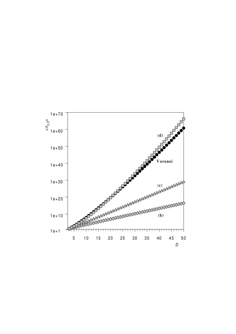
Figure 5: The average number of vertices in a $D$ dimensional Voronoï cell generated from Poissonian points can be exactly calculated [32] (black circles). Here this number is compared with the one associated with the fixed point structures (gray symbols).

(Note that for $D=3$ Eq.(25) give $\langle n_{0,D}\rangle=96\pi^{2}/35$ that substituted into Eq.( 26) leads to $X_{3}=2+48\pi^{2}/35=15.53...$). By substituting the fixed point configuration into (26) we find that the structure (b) has $\langle n_{0,D}\rangle=(D+1)2^{D-1}$, the structure (c) gives $\langle n_{0,D}\rangle=(2D)!(D!)^{-2}$, whereas (d) has $\langle n_{0,D}\rangle=(D+1)!$. In figure (5) the behaviors of the average number of vertices per cell in the Voronoï froth and in the three structures (b), (c) and (d) is shown for $3\leq D\leq 50$.

6 Conclusions

The topological structure of a $D$-dimensional cellular system can be characterized, in average, in terms of the coordinations ($X_{k}$) of the irregular polytopes which are making the structure (Section 2). Only the coordinations of the even dimensional polytopes ($X_{2l}$) are necessary for this characterization, the odd ones are expressed in terms of the even ones by the relation (4). Therefore, the average structure of a $D$-dimensional froth is characterized by a sequence $\{X_{2},X_{4},X_{6}.....\}$ of ${D\over 2}-1$ (or ${D-1\over 2}$) variables for $D$ even (or odd). These variables are related with the space-curvature through Eq.(5). Regions in the parameter space $\{X_{2l}\}$ corresponding to $D$-dimensional froths tiling spaces of different curvature are discussed for $D\leq 4$ (fig(1) and Eqs.(6) and (7)).

We use cell division and coalescence transformations to build $D$-dimensional froths (Section 3). We show that through cell-division/coalescence transformations it is possible to generate the entire class of froths tiling topologically identical manifolds. The dynamical renormalization of the variables $X_{k}$ under such transformations is found (Eq.(11)). The existence of classes of structures which are invariant (fixed points) under cell division/coalescence is pointed out (Eqs.(12) and (13) ). We show that these structures are tiling Euclidean spaces.

Several fixed point Euclidean structures are constructed in Section 5. We discuss the average statistical properties for the of minimally coordinated Euclidean froths, and for several topologically homogeneous space partitions (Eqs(20-24) and tab.(1)). The topological properties of the most homogeneous cellular partition are searched and compared with known geometrical results (fig.(3)).

Finally, the fixed point Euclidean structures are compared with known high dimensional structures generated by sphere packings and Voronoï constructions (figs.(4) and (5)).

Acknowledgements

A special thank to Nicolas Rivier for many discussions and comments which have highly contributed to the research and have improved the presentation of the work. I acknowledge discussions with J. F. Wheather and D. Sherrington. This work was partially supported from the European Union Marie Curie fellowship (TMR ERBFMBICT950380).

Appendix A The existence of polytopes $\{5,3,...\}$ up to $D=4$

There is a class of regular polytopes with $X_{2}=5$ and minimally connected vertices ($\{5,3,...\}$) which exists up to dimension $D=4$ [26].

They are pentagons in $D=2$, dodecahedra ($\{5,3\}$) in $D=3$ and polytopes $\{5,3,3\}$ in $D=4$. A tessellation of pentagons makes a $2D$ elliptic froth with $X_{2}=5$ and $C_{2}=12$, it is a dodecahedron $\{5,3\}$. A tessellation of dodecahedra make a $3D$ elliptic froths with $X_{2}=5$, $X_{3}=12$, $C_{3}=120$, which is the $\{5,3,3\}$ structure. It turns out that a tessellation with $\{5,3,3\}$ polytopes does not makes any 5-dimensional polytope [26]. If existing, such a structure would be a 4-dimensional polytope with $X_{2}=5$, $X_{3}=12$, $X_{4}=120$. By substituting these values into Eq.(7), we get $C_{4}=\chi_{4}$, which implies $\chi_{4}>0$. This hypothetical structure would therefore be an elliptic froth, homotrope to a sphere which implies $\chi_{4}=2$. Then, from the previous identity, $C_{4}=2$. The hypothetical $\{5,3,3,3\}$ structure would be an elliptic froths which closes onto itself with two cells only. But two cells are insufficient to make a 5-dimensional polytope (the minimum number is 6). It follows therefore that the $\{5,3,3,3\}$ structure does not exists and neither exist the others higher dimensional tessellations $\{5,3,3,3...\}$.

	Ideal	FP {5,3,…} (a)		FP {4,3,…} (b)		FP (c)		FP (d)
	$X_{2}^{ideal}$	$X_{2}^{*}$	$X_{D}^{*}$	$X_{2}^{*}$	$X_{D}^{*}$	$X_{2}^{*}$	$X_{D}^{*}$	$X_{2}^{*}$	$X_{D}^{*}$
$D$		$5{D(D+1)\over(D-1)(D+3)}$	$4{D(D+1)\over(D-1)(D+2)}$	$\scriptstyle 4D-2$		$2{2D-1\over D-1}$	$\scriptstyle D(D+1)$	$12{D\over 3D-2}$	$\scriptstyle 2^{D+1}-2$
3	5.1043	5	12	4.8	10	5	12	5.1458	14
4	4.7668	4.7619	26	4.4444	14	4.6667	20	4.8	30
5	4.5881	4.6875	242	4.2857	18	4.5	30	4.6154	62
6	4.7728			4.2	22	4.4	42	4.5	126
7	4.4017			4.1481	26	4.3333	56	4.4211	254
8	4.3468			4.1143	30	4.2857	72	4.3636	510
9	4.3052			4.0909	34	4.25	90	4.32	1022
10	4.2724			4.0747	38	4.2222	110	4.2857	2046

Table 1: Average ring coordination ($X_{2}$) and cell coordination ($X_{D}$) for some Euclidean fixed point structures (FP) generated by cell division (see text).

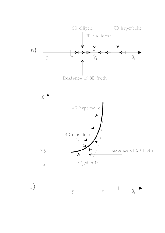
Figure 1: Different regions in the parameter space $\{X_{2l}\}$ corresponds to froths which are tiling spaces of different curvatures. (a) two dimensional froths with $X_{2}<6$ tile elliptic surfaces, froths with $X_{2}>6$ tile hyperbolic surfaces and $X_{2}=6$ corresponds to froths tiling the Euclidean plane. (b) The hyperbolic, Euclidean and elliptic tilings corresponds to three regions of the $\{X_{2},X_{4}\}$ parameter space. Cell division transformations modify the properties of curved tilings towards the Euclidean ones (arrows).

Figure 2: Given two different partitions of the $D$-dimensional space in $D$-simplices one can be transformed into the other by a finite sequence of two local transformations called “Alexander moves” ((a) and (b) for the two dimensional case). In the dual froths these transformations corresponds to two special cell division transformations ((c) and (d) for the two dimensional case)

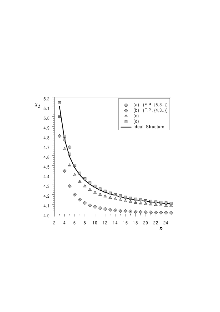
Figure 3: The average ring connectivity $X_{2}$, for homogeneous partitions of spaces of dimension $D$, obtained from a geometrical approach [25] (full line) is compared with the one of the fixed point structures (symbols).

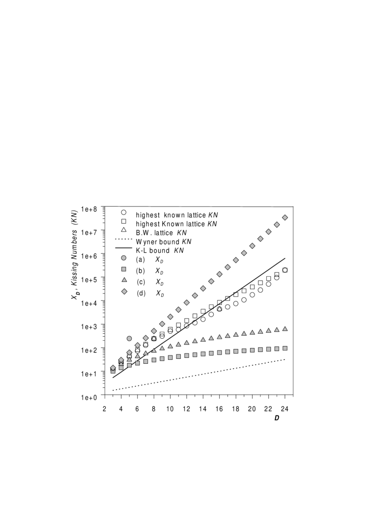
Figure 4: Kissing Numbers KN (maximum number of identical hard spheres that can stay around and touch a given sphere in $D$ dimensions) and coordination numbers $X_{D}$ (average number of cells around a given cell in a $D$ dimensional froth) are compared for some known sphere packings (open symbols) and for the fixed point structures (full symbols). Two upper and lower bounds for the KN in high dimensions are also plotted (full and dotted lines).

References

- [1] D’A.W. Thompson, On Growth and Form Cambridge Univ. Press. (1917, 1942), ch.7.
- [2] D. Weaire and N. Rivier, Contemp. Physics 25 (1984) 59.
- [3] J. Stavans, Rep. Prog. Mod. Phys. 56 (1993) 733.
- [4] H.V. Atkinson, Acta metall 36 (1988) 469-491.
- [5] C.S. Smith, Metal Interfaces (ASM Cleveland OH, 1952) 65. C.S. Smith, Rev. mod. Phys. (April 1964) 524.
- [6] J. Stavans, Physica A 194 (1993) 307-314.
- [7] J.C.M. Mombach, M.A.Z. Vasconcellos and R.M.C. de Almeida, J. Phys. D Appl. Phys. 23 (1990) 600-606.
- [8] B. Dubertret and N. Rivier, Biophysical Journal 73 (1997) 38-44.
- [9] G. Voronoi, J. reine angew. Math. 134 (1908) 198.
- [10] J.F. Sadoc and R. Mosseri, Frustration Géométrique (Ed. Eyrolles, Paris 1997).
- [11] M.O’Keeffe and B.G.Hyde, Crystal Structures (MSA, Washington 1996).
- [12] Von B.L. van der Waerden, Die Naturwissenschaften 7 (1961) 189.
- [13] J.H. Conway and N.J.A. Sloane, Sphere Packings, Lattices and Groups, (Springer-Verlag, 1988).
- [14] E. Gardner, J. Phys. A: Math. Gen. 21 (1988) 257-270.
- [15] E. Gardner and B. Derrida, J. Phys. A: Math. Gen. 21 (1988) 271.
- [16] N. Brunel, J-P. Nadal and G. Toulouse, J. Phys. A: Math. Gen. 25 (1992) 5017-5037.
- [17] D.J. Amit, Modeling Brain Function (Cambridge Univ. Press. 1989).
- [18] J. Kurchan and L. Laloux, cond-mat/9510079 (1995).
- [19] N.H. Christ, R. Friedberg and T.D. Lee, Nuclear Physics B 202 (1982) 89-125.
- [20] F. David, Lect. given at Les Houches Nato ASI Fluctuating Geometries in Statistical Mechanics and Field Theory 1994.
- [21] J. Ambjorn, Lect. given at Les Houches Nato ASI Fluctuating Geometries in Statistical Mechanics and Field Theory 1994.
- [22] J. Ambjorn, J. Jurkiewicz and Y. Watabiki, hep-th/9503108 (1995).
- [23] J. Ambjorn, M. Canfora and A. Marzuoli, hep-th/9612069 (1996).
- [24] J. F. Wheather, J. Phys. A.: Math. Gen. 27 (1994) 3323-3353.
- [25] T. Aste, N. Rivier, J. Phys. A28 (1995) 1381-98
- [26] H.S.M. Coxeter. Regular Polytopes. (Dover, New York, 1973). H.S.M. Coxeter. Introduction to Geometry. (J. Wiley and Sons, New York, 1961).
- [27] J. W. Alexander, Ann. Math. 31 (1930) 292.
- [28] F.T. Lewis, Proc. Am. Acad. Arts. Sci. 58 (1923) p.537-52; The Anatomical Record 50 (1931) p.235-65; Am. J. Bot. 37 (1950) p.715-21.
- [29] K.J. Dormer, “Fundamental tissue geometry for biologists”, (Cambridge Univ. Press. 1980).
- [30] W. Thomson (Lord Kelvin), Phil. Mag. 24 (5) (1887) 503.
- [31] W. Thomson (Lord Kelvin), republished in The Kelvin Problem, D. Weaire Ed. (Taylor & Francis 1996) 21.
- [32] L. Oger, A. Gervois, J. P. Toadec and N. Rivier, Phil. Mag. B 74 (1996) 177-197.
- [33] F. C. Frank and J. S. Kasper, Acta crystallogr. 12 (1959) 483.
- [34] E. B. Matzke, Am. J. Bot. 33 (1946) p.58-80.
- [35] J.L. Meijering, Philips Res. Rep. 8 (1953) 270.
- [36] C. Itzykson and J.M. Drouffe, Statistical Field Theory (Cambridge University Press 1988) vol.2, chap.11 .