Density of states of a two-dimensional electron gas in a non-quantizing magnetic field

Abstract

We study local density of electron states of a two-dimentional conductor with a smooth disorder potential in a non-quantizing magnetic field, which does not cause the standart de Haas-van Alphen oscillations. It is found, that despite the influence of such “classical” magnetic field on the average electron density of states (DOS) is negligibly small, it does produce a significant effect on the DOS correlations. The corresponding correlation function exhibits oscillations with the characteristic period of cyclotron quantum $\hbar\omega_{c}$.

I Introduction

In the clean homogeneous electron gas the wave functions of electrons are plane waves and the density of electron gas is constant in space. In disordered conductors electrons are scattered by impurities, which change their wave functions from the plane waves. This, in turn, results in spatial variations of the electron density. It is appropriate to describe those variations by introducing the local density of electron states, $\nu(\epsilon,{\bf r})$, which is determined by the equation

$$\nu(\epsilon,{\bf r})=2\sum_{\alpha}\left|\psi_{\alpha}({\bf r})\right|^{2}\delta(\epsilon-\epsilon_{\alpha}),$$ (1)

where index $\alpha$ specifies the electronic states, and the factor of two reflects the spin degeneracy. The distribution function of the local DOS at the fixed energy in open metallic disordered samples was studied in many papers (see e.g. [3]) with the emphasis on the rare, nontypical fluctuations. It was found that although the local DOS distribution is close to the Gaussian one, it has slowly decaying logarithmically normal asymptotics. Prigodin[4] studied correlation function of the density of the electron states of a two-dimensional system at different energies in relation to the NMR line shape.

It is well-known that strong magnetic field modifies the single-particle density of electron states, both local and average, due to the Landau quantization. In a two-dimensional electron gas the quantization leads to a peak structure in the average density of states, which is revealed in tunneling experiments as peaks in the dependence of the tunneling conductance on the applied bias, see, e.g., Ref. [5]. The form and width of these peaks are determined[6] by the disorder.

In a weak magnetic field the distance between the Landau levels, $\hbar\omega_{c}$, is smaller than their disorder-induced width. As a result, in such “classical” magnetic field, oscillations in the average density of states caused by the Landau quantization become exponentially small [6], $\propto\exp[-2\pi/(\omega_{c}\tau_{s})]$. Here $\tau_{s}$ is a quantum lifetime of an electron.

The goal of the present paper is to show that, despite such “classical” magnetic field does not influence the average DOS, it does produce a significant effect on the correlation function of the local density of states fluctuations

$$P(\epsilon_{1},\epsilon_{2},{\bf r})={\left<\delta\nu(\epsilon_{1},{\bf r})\delta\nu(\epsilon_{2},{\bf r})\right>\over\nu_{0}^{2}}.$$ (2)

Here $\delta\nu(\epsilon,{\bf r})=\nu(\epsilon,{\bf r})-\nu_{0}$ is the local deviation of the DOS in point ${\bf r}$ from its average value, $\nu_{0}=m/\pi\hbar^{2}$, $m$ is the electron mass, and brackets $\left<\mbox{ }\right>$ denote averaging over the random impurity potential. Clearly, the correlation function depends only on difference of energy agruments, $P(\epsilon_{1},\epsilon_{2},{\bf r})=P(\epsilon_{1}-\epsilon_{2},{\bf r})$.

The effect of the classical magnetic field on the DOS correlation function becomes pronounced if the disorder potential has a correlation length much larger than the Fermi wave length. In such a potential, electrons experience small-angle scattering, and their transport relaxation time $\tau_{\rm tr}$, is much larger than $\tau_{s}$. Thus there exists a range of magnetic fields, in which Landau quantization is suppressed ($\omega_{c}\tau_{s}\ll 1$), while classical electron trajectories are strongly affected by the field ($\omega_{c}\tau_{\rm tr}\gg 1$). In this regime the correlation function, $P(\epsilon_{1}-\epsilon_{2})$ is strongly enhanced with respect to the zero magnetic field case and exhibits peaks as a function of energy difference $\epsilon_{1}-\epsilon_{2}$ with the distance between peaks equal to the cyclotron quantum, $\hbar\omega_{c}$. For the macroscopically homogeneous sample the shape of the $n$-th peak, $|(\epsilon_{1}-\epsilon_{2})-n\hbar\omega_{c}|\lesssim\hbar\omega_{c}/2$, in the local DOS correlation function is given by:

$$P(\epsilon_{1}-\epsilon_{2})={\omega_{c}^{2}\tau_{tr}^{2}\over 2\sqrt{2}\pi E_{F}\tau_{tr}}\,{1\over n}\,f\!\left({\epsilon_{1}-\epsilon_{2}-n\hbar\omega_{c}\over\hbar n^{2}/\tau_{\rm tr}}\right),$$ (3)

where

$$f(x)={1\over\sqrt{2}}\left[{1+\sqrt{x^{2}+1}\over x^{2}+1}\right]^{1/2},$$ (4)

and $E_{F}$ is the Fermi energy. As $n$ gets bigger, the width of the peaks increases and their height decreases, so that eventually the oscillatory structure is washed out. The total number of resolved peaks is of the order of $\sqrt{\omega_{c}\tau_{\rm tr}}$.

Sensitivity of the correlation function $P$ to the classical magnetic field comes from the fact, that this function is directly associated with the self-crossing of classical electron trajectories. We denote the probability for an electron to complete a loop of self-crossing trajectory over time $t$ as $K(t)$. The correlation function, $P(\epsilon_{1}-\epsilon_{2})$, turns out to be proportional to the Fourier transform of this return probability,

$$P(\epsilon_{1}-\epsilon_{2})\propto K(\epsilon_{1}-\epsilon_{2})=\int_{0}^{\infty}dte^{-i(\epsilon_{1}-\epsilon_{2})t}K(t).$$

The strong enough, $\omega_{c}\tau_{\rm tr}\gg 1$, magnetic field curves the electron trajectories, significantly affects the return probability and, in turn, leads to specific correlations in the local DOS at $\epsilon_{1}-\epsilon_{2}\approx\hbar\omega_{c}$.

For long time scales $t\gg\tau_{\rm tr}$, the function $K(t)$ can be found from the diffusion equation. It gives $K(t)\propto(Dt)^{-1}$ for the two-dimensional case ($D$ is the diffusion coefficient). The Fourier transform, $K(\omega)$, is proportional to $\ln(\omega)$, which leads to the well-known[4] logarithmic form of the local DOS correlation function with the renormalized by the magnetic field diffusion coefficient.

At short time scales, $t\ll\tau_{\rm tr}$, electrons move ballistically along the cyclotron orbits. Provided that $\omega_{c}\tau_{\rm tr}\gg 1$, during the time $t$ electron may return to the initial point many times. Multiple periodic returns of electron produce peaks in the probability Fourier transform $K(\omega)$ at energies, which are multiples of the cyclotron quantum. Correlation function $P(\epsilon_{1}-\epsilon_{2})$ oscillates with the same period, which is reflected by Eq. (3).

II Derivation of the DOS correlation function

Now we derive expression for the correlation function of the local DOS, $P$, valid for arbitrary electron energies. We omit the Planck constant in all the intermediate formulas. The DOS, Eq. (1), can be rewritten in terms of the exact retarded and advanced Green’s functions of an electron in the following way:

$$\nu(\epsilon,{\bf r})={1\over\pi i}\left[{\cal G}^{A}_{\epsilon}({\bf r},{\bf r})-{\cal G}^{R}_{\epsilon}({\bf r},{\bf r})\right],$$ (5)

where

$${\cal G}^{R}_{\epsilon}({\bf r}_{1},{\bf r}_{2})=\sum_{\alpha}{\psi_{\alpha}^{*}({\bf r}_{1})\psi_{\alpha}({\bf r}_{2})\over\epsilon-\epsilon_{\alpha}+i0},$$ (6)

and ${\cal G}^{A}_{\epsilon}({\bf r}_{1},{\bf r}_{2})=[{\cal G}^{R}_{\epsilon}({\bf r}_{2},{\bf r}_{1})]^{*}$. Single electron wave functions $\psi_{\alpha}({\bf r})$ satisfy the Schrödinger equation for noninteracting electrons, $\hat{H}_{0}\psi_{\alpha}=(\epsilon_{\alpha}+E_{F})\psi_{\alpha}$, where $\hat{H}_{0}=-(\hbar^{2}/2m)\nabla^{2}+U_{r}({\bf r})$, and $U_{r}({\bf r})$ is the random potential.

With the help of Eq. (5), the DOS correlation function, Eq. (2), can be rewritten in terms of the ensemble-averaged products of the electron Green’s functions:

$$P(\epsilon_{1}-\epsilon_{2},{\bf r}) = {1\over(\pi\nu_{0})^{2}}\left[2{\bf Re}\left<{\cal G}^{R}_{\epsilon_{1}}({\bf r},{\bf r}){\cal G}^{A}_{\epsilon_{2}}({\bf r},{\bf r})\right>\right.$$ (7)

$$+ \left<{\cal G}^{R}_{\epsilon_{1}}({\bf r},{\bf r}){\cal G}^{R}_{\epsilon_{2}}({\bf r},{\bf r})\right>\!\!+\!\!\left.\left<{\cal G}^{A}_{\epsilon_{1}}({\bf r},{\bf r}){\cal G}^{A}_{\epsilon_{2}}({\bf r},{\bf r})\right>\right].$$ (8)

The averages of the type $\left<{\cal G}^{R}{\cal G}^{R}\right>$ and $\left<{\cal G}^{A}{\cal G}^{A}\right>$ can be neglected as they do not contain contributions associated with the electron trajectories longer than $\lambda_{F}$ and, thus, do not produce energy dependence of $P(\epsilon_{1}-\epsilon_{2},{\bf r})$ at $\epsilon_{1}-\epsilon_{2}\ll E_{F}$. To the contrary, averaged product $\left<{\cal G}^{R}{\cal G}^{A}\right>$ is determined by long electron trajectories (see e.g. Ref. [7]). In general, the product of two exact Green’s functions ${\cal G}^{R}_{\epsilon_{1}}({\bf r}_{1},{\bf r}_{2}){\cal G}^{A}_{\epsilon_{2}}({\bf r}_{3},{\bf r}_{4})$ oscillates rapidly with the distance between its arguments, so that the function

$$K(\epsilon_{1},\epsilon_{2},{\bf r}_{1},{\bf r}_{2},{\bf r}_{3},{\bf r}_{4})=\left<{\cal G}^{R}_{\epsilon_{1}}({\bf r}_{1},{\bf r}_{2}){\cal G}^{A}_{\epsilon_{2}}({\bf r}_{3},{\bf r}_{4})\right>$$ (10)

averages out. This is no longer the case if its arguments are close to each other pairwise. Namely, the sizes $|{\bf r}_{1}-{\bf r}_{4}|,\,|{\bf r}_{2}-{\bf r}_{3}|$ or, alternatively, $|{\bf r}_{1}-{\bf r}_{3}|,\,|{\bf r}_{2}-{\bf r}_{4}|$ of spatial domains defining the ends of a trajectory should be small enough (less than $v_{F}\tau_{s}$) so that electron propagation in these two domains could be described by plane waves.

If the ends of trajectories are separated by the distance exceeding electron wave-length, $|{\bf r}_{1}-{\bf r}_{2}|\gtrsim\lambda_{F}$, one can relate the function $K$ to the generalized classical correlation functions – diffuson ${\cal K}^{\cal D}$ and Cooperon ${\cal K}^{\cal C}$, which are given by the sum of all ladder and all maximally-crossed diagrams respectively. Namely,

$$K(\epsilon_{1},\epsilon_{2},{\bf r}_{1}, {\bf r}_{2}, {\bf r}_{3},{\bf r}_{4})$$ (11)

$$= \pi\nu_{0}\int{d\phi_{1}\over 2\pi}\int{d\phi_{2}\over 2\pi}e^{i{\bf p}_{1}({\bf r}_{1}-{\bf r}_{4})}$$ (12)

$$\times e^{i{\bf p}_{2}({\bf r}_{3}-{\bf r}_{2})}{\cal K}^{\cal D}_{\epsilon_{1}-\epsilon_{2}}({\bf r}_{1},\phi_{1};{\bf r}_{2},\phi_{2})$$ (13)

$$|{\bf r}_{1}-{\bf r}_{4}|,|{\bf r}_{2} - {\bf r}_{3}|\ll v_{F}\tau_{s}$$ (14)

or

$$K(\epsilon_{1},\epsilon_{2},{\bf r}_{1}, {\bf r}_{2}, {\bf r}_{3},{\bf r}_{4})$$ (15)

$$= \pi\nu_{0}\int{d\phi_{1}\over 2\pi}\int{d\phi_{2}\over 2\pi}e^{i{\bf p}_{1}({\bf r}_{1}-{\bf r}_{3})}$$ (16)

$$\times e^{i{\bf p}_{2}({\bf r}_{4}-{\bf r}_{2})}{\cal K}^{\cal C}_{\epsilon_{1}-\epsilon_{2}}({\bf r}_{1},\phi_{1};{\bf r}_{2},\phi_{2})$$ (17)

$$|{\bf r}_{1}-{\bf r}_{3}|,|{\bf r}_{2} - {\bf r}_{4}|\ll v_{F}\tau_{s}.$$ (18)

Here ${\bf p}_{i}=p_{F}{\bf n}_{i}$, where ${\bf n}_{i}=(\cos\phi_{i},\sin\phi_{i})$ is a unit vertor with the direction determined by the angle $\phi_{i}$.

In the opposite limit, when the all four points ${\bf r}_{1}$, ${\bf r}_{2}$, ${\bf r}_{3}$, and ${\bf r}_{4}$ coinside, both ladder and maximally-crossed diagrams contribute to Eq. (10). As a result, the DOS correlation function, Eq. (7), contains both the diffuson and the Cooperon contributions:

$$P(\epsilon_{1},\epsilon_{2},{\bf r})={2\over\pi\nu_{0}}\,{\bf Re}\left[{\cal D}_{\epsilon_{1}-\epsilon_{2}}({\bf r},{\bf r})+{\cal C}_{\epsilon_{1}-\epsilon_{2}}({\bf r},{\bf r})\right].$$ (19)

Here ${\cal D}$ and ${\cal C}$ are the diffuson, ${\cal K}^{\cal D}$ and the Cooperon, ${\cal K}^{\cal C}$, averaged over the initial and the final directions of the electron momentum:

$${\cal D}_{\epsilon_{1}-\epsilon_{2}}({\bf r}_{1},{\bf r}_{2}) = \int{d\phi_{1}\over 2\pi}{d\phi_{2}\over 2\pi}{\cal K}^{\cal D}_{\epsilon_{1}-\epsilon_{2}}({\bf r}_{1},\phi_{1};{\bf r}_{2},\phi_{2}),$$ (20)

$${\cal C}_{\epsilon_{1}-\epsilon_{2}}({\bf r}_{1},{\bf r}_{2}) = \int{d\phi_{1}\over 2\pi}{d\phi_{2}\over 2\pi}{\cal K}^{\cal C}_{\epsilon_{1}-\epsilon_{2}}({\bf r}_{1},\phi_{1};{\bf r}_{2},\phi_{2}).$$ (21)

As one sees, calculation of the DOS correlation function reduces to the analysis of two classical correlation functions, ${\cal D}$ and ${\cal C}$. Provided that we are interested in the DOS correlation function in the presence of the magnetic field, the problem can be further simplified. Indeed, as it is well-known, the diffusion and the Cooperon depend quite differently on the magnetic field (see e. g. Ref. [8]). In particular, ${\cal C}$ is exponentially suppressed if the magnetic length, $\lambda_{H}=\sqrt{c\hbar/eH}$, becomes smaller than the transport relaxation length $l_{tr}$. We, in fact, assumed a much stronger condition, $\omega_{c}\tau_{tr}\gg 1$, for the magnetic field. Thus the Cooperon term in Eq. (19) can be neglected in our case. On the other hand, the diffusion term in Eq. (19) is meaningful and will be analyzed below.

III DOS correlation function for an infinite two-dimensional electron gas

Let us first calculate the local DOS correlation function, $P(\epsilon_{1}-\epsilon_{2})$, in the macroscopically homogeneous sample. The generalized diffuson, ${\cal K}^{\cal D}_{\omega}({\bf r}_{1},\phi_{1};{\bf r}_{2},\phi_{2})$, satisfies the Boltzmann equation (see e.g. Ref.[7]) describing the scattering of electrons on impurities in the presence of the magnetic field. In the special case $\tau_{s}\ll\tau_{\rm tr}$ we are interested in, small angles scattering dominates the collision integral. With account for this simplification, the transport equation for ${\cal K}^{\cal D}_{\omega}({\bf r}_{1},\phi_{1};{\bf r}_{2},\phi_{2})$ takes the Fokker-Planck form:

$$\Big{[}-i\omega + v_{F}{\bf n}_{2}{\partial\over\partial{\bf r}_{2}}+\omega_{c}{\partial\over\partial\phi_{2}}-{1\over\tau_{\rm tr}}{\partial^{2}\over\partial\phi_{2}^{2}}\Big{]}{\cal K}^{\cal D}_{\omega}({\bf r}_{1},\phi_{1};{\bf r}_{2},\phi_{2})$$ (22)

$$= 2\pi\delta(\phi_{1}-\phi_{2})\,\delta({\bf r}_{1}-{\bf r}_{2}).$$ (23)

Equation (22) describes electron motion along the cyclotron orbit accompanied by the angular diffusion caused by scattering on a random potential. The solution of this equation will give us the Fourier transform,

$${\cal K}^{\cal D}_{\omega}(1;2)=\int_{0}^{\infty}{\cal K}^{\cal D}(t,1;2)e^{-i\omega t}dt$$

of probability density, ${\cal K}^{\cal D}(t,{\bf r}_{1},\phi_{1};{\bf r}_{2},\phi_{2})$, for electron which starts at moment $t=0$ in point ${\bf r}_{1}$ with the direction of momentum $\phi_{1}$ to arrive at moment $t$ to the point ${\bf r}_{2}$ with momentum direction $\phi_{2}$.

In order to solve Eq. (22) it is convenient to introduce new spatial variables which correspond to the center of the electron cyclotron orbit:

$${\bf R}={\bf r}+R_{c}[{\bf n}\times{\bf z}].$$ (24)

Here $R_{c}$ is a cyclotron radius, and ${\bf z}$ is a unit vector parallel to the magnetic field. Changing variables in Eq. (22), and performing the Fourier transformation from ${\bf R}_{2}$ to ${\bf q}$, we obtain:

$$\Biggl{\{} -i \omega+\omega_{c}{\partial\over\partial\phi_{2}}+{R_{c}^{2}q^{2}\over 2\tau_{\rm tr}}-{1\over\tau_{tr}}{\partial^{2}\over\partial\phi_{2}^{2}}$$ (25)

$$+ {R_{c}^{2}\over\tau_{\rm tr}}\left[({\bf n}_{2}{\bf q})^{2}-{q^{2}\over 2}-{i\over R_{c}}\left({\bf n}_{2}{\bf q}{\partial\over\partial\phi_{2}}+{\partial\over\partial\phi_{2}}{\bf n}_{2}{\bf q}\right)\right]\Biggr{\}}$$ (26)

$$\times {\cal K}^{\cal D}_{\omega}({\bf R}_{1},\phi_{1};{\bf q},\phi_{2})=2\pi\delta(\phi_{1}-\phi_{2})e^{-i{\bf q}{\bf R_{1}}}.$$ (27)

We seek for the solution of Eq. (25) in the following form:

$${\cal K}^{\cal D}_{\omega}({\bf R}_{1},\phi_{1};{\bf q},\phi_{2})=\sum_{n}e^{in\phi_{2}}F_{n}(\omega,{\bf q};\phi_{1}).$$ (28)

Substitution of Eq.(28) to Eq. (25) results in a linear system of equations for $F_{n}$. At small enough wave vectors, $qR_{c}\ll\omega_{c}^{2}\tau_{\rm tr}/(|\omega|+\omega_{c})$, terms in the square brackets in the l.h.s. of Eq. (25) become small, the equations corresponding to different $n$ become independent, and we obtain a solution for $F_{n}(\omega,{\bf q};\phi_{1})$ in the form:

$$F_{n}(\omega,{\bf q};\phi_{1})={e^{-in\phi_{1}}e^{-i{\bf q}{\bf R}_{1}}\over\displaystyle-i(\omega-n\omega_{c})+{R_{c}^{2}q^{2}\over 2\tau_{\rm tr}}+{n^{2}\over\tau_{\rm tr}}}.$$ (29)

The inverse transformation of variables immediately yields now the solution of Eq. (22):

$${\cal K}^{\cal D}_{\omega}({\bf r}_{1},\phi_{1};{\bf r}_{2},\phi_{2}) = \int{d{\bf q}\over(2\pi)^{2}}e^{i{\bf q}({\bf r}_{2}-{\bf r}_{1})}$$ (30)

$$\times \sum_{n}{e^{in(\phi_{2}-\phi_{1})}e^{iR_{c}{\bf q}[({\bf n}_{2}-{\bf n}_{1})\times{\bf z}]}\over\displaystyle-i(\omega-n\omega_{c})+{R_{c}^{2}q^{2}\over 2\tau_{\rm tr}}+{n^{2}\over\tau_{\rm tr}}}.$$ (31)

After substitution of Eq. (30) into the Eqs. (19) and (20), and subsequent integration over angles, we obtain the following expression for the correlation function of the local DOS of a homogeneous two-dimensional conductor in the classical magnetic field:

$$P(\epsilon_{1}-\epsilon_{2}) = {2\over\pi\nu_{0}}\,\int{d{\bf q}\over(2\pi)^{2}}{\bf Re}\,{\cal D}_{\epsilon_{1}-\epsilon_{2}}({\bf q}),$$ (32)

$${\cal D}_{\epsilon_{1}-\epsilon_{2}}({\bf q}) = \sum_{n}{|J_{n}(qR_{c})|^{2}\over\displaystyle-i(\epsilon_{1}\!-\!\epsilon_{2}\!-\!n\omega_{c})\!+{R_{c}^{2}q^{2}\over 2\tau_{\rm tr}}+{n^{2}\over\tau_{\rm tr}}}.$$ (33)

Here $J_{n}(z)$ is a Bessel function. At small frequencies, $\omega=\epsilon_{1}-\epsilon_{2}\ll\hbar/\tau_{\rm tr}$, the $n=0$ term in Eq. (33) dominates, and

$${\cal D}_{\omega}({\bf q})\approx{1\over-i\omega+R_{c}^{2}q^{2}/2\tau_{\rm tr}}.$$

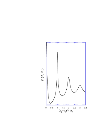
FIG. 1.: Energy dependence of the local density of states correlation function, $P(\epsilon_{1}-\epsilon_{2})$, of the macroscopically homogeneous sample in the classical magnetic field, obtained by numerical analysis of Eqs. (32)-(33). Parameter $\omega_{c}\tau_{tr}=10$.

This limit corresponds to the diffusion regime with the diffusion coefficient $D=R_{c}^{2}/2\tau_{tr}$ renormalized by the magnetic field. The correlation function $P(\epsilon_{1}-\epsilon_{2})$ depends logarithmically on $\epsilon_{1}-\epsilon_{2}$ in this limit:

$$P(\epsilon_{1}-\epsilon_{2})={(\omega_{c}\tau_{tr})^{2}\over 2\pi E_{F}\tau_{tr}}\ln\left[{\hbar\over|\epsilon_{1}-\epsilon_{2}|\tau_{tr}}\right].$$ (34)

At large frequencies, $\omega=\epsilon_{1}-\epsilon_{2}\gg\hbar/\tau_{\rm tr}$ the correlation function $P(\epsilon_{1}-\epsilon_{2})$ exhibits peaks at $\epsilon_{1}-\epsilon_{2}$ close to multiples of cyclotron quantum, $n\hbar\omega_{c}$. The form of the n-th peak is given by:

$$P(\epsilon_{1}-\epsilon_{2})={\omega_{c}^{2}\tau_{tr}^{2}\over\pi E_{F}\tau_{tr}}{\bf Re}\left\{I_{n}[a(n,\delta\omega)]K_{n}[a(n,\delta\omega)]\right\},$$ (35)

where $\hbar\delta\omega=\epsilon_{1}-\epsilon_{2}-n\hbar\omega_{c}$ was introduced instead of $\epsilon_{1}-\epsilon_{2}$, and $a(n,\delta\omega)=2(n^{2}-i\delta\omega\tau_{tr})$. Functions $I_{n}(a)$ and $K_{n}(a)$ are the modified Bessel functions. For large $a$ we can use the asymptotical relation, $I_{n}(a)K_{n}(a)\approx 1/2a$, and arrive at the resulting Eq. (3) that describes energy dependence of the local DOS correlation function in the vicinity of $n-$th peak.

Overall energy dependence of the correlation function of the local density of states for an infinite sample, obtained by numerical analysis of Eqs. (32)-(33) is presented in Fig. 1. The DOS correlation function exhibits strong oscillations with the period close to $\hbar\omega_{c}$.

IV Oscillations of the DOS for tunneling into the edge of a two-dimensional electron gas

The tunneling density of states $\nu(\epsilon,{\bf r})$ is directly related to the tunneling differential conductance $G(V)$ of a point contact attached to the two-dimensional gas, $\nu(eV,{\bf r})/\nu_{0}=G(V)/G_{0}$ (here $G_{0}$ is the average linear conductance at zero magnetic field). Thus measuring the conductance correlation function $\left<\delta G(V)\delta G(V+\Delta V)\right>$ one can determine the DOS correlation function, $P(e\Delta V)=\left<\delta G(V)\delta G(V+\Delta V)\right>/G_{0}^{2}$. Here $\delta G(V)=G(V)-G_{0}$. The tunneling DOS we studied so far is related to tunneling into the “bulk” of a two-dimensional electron gas, see Fig. 2a. For GaAs heterostructures, however, there exists a well developed method of forming point contacts for lateral tunneling into the edge of a two-dimensional electron gas (see, e.g., the review of Beenakker and van Houten, Ref.[9]). The edge affects electron trajectories and thus alters the correlation function of the tunneling density of states. Below we estimate $P(\epsilon_{1}-\epsilon_{2})$ for the specific case of lateral tunneling, schematically shown in Fig. 2b. We demonstrate that the oscillatory pattern of $P$ at energies larger than $\hbar\omega_{c}$ persists, although the amplitude of oscillations becomes smaller than in the case of tunneling into the bulk.

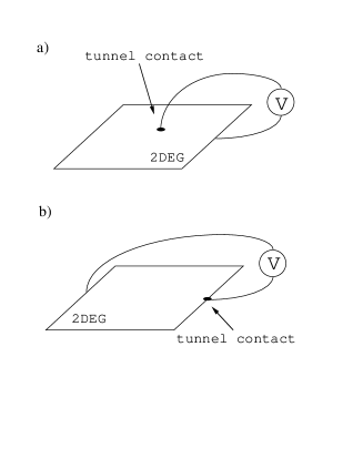
FIG. 2.: Two possible tunneling experiment that enable to measure properties of the tunneling density of electron states: (a) the point-like tunnel contact is attached to a two-dimensional conductor far from its edges; (b) tunneling occurs at the edge of the two-dimensional electron gas.

In order to find the conductance correlation function, one should, according to Eq. (19), find the Fourier transform of the return probability, ${\cal D}(t)$, for an electron emitted from the contact right at the edge of the electron gas.

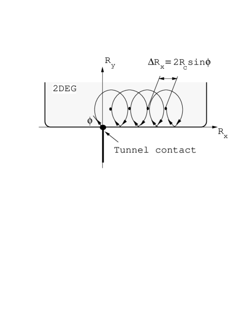
FIG. 3.: Drift of an electron in the magnetic field caused by the multiple specular reflections from the boundary of the two-dimensional electron gas.

Let us consider an electron which is emitted from a point-like tunnel contact attached to the edge of the two-dimensional conductor at a moment $t=0$ with the initial velocity characterized by the angle $\phi_{1}$. For any nonzero $\phi_{1}$ electron experiences multiple reflections from the boundary of the two-dimensional electron gas (see Fig. 3). The boundary of the electron gas is usually smooth, so that we assume this scattering to be purely specular. Those multiple scattering events lead to a drift of the guiding center of electron orbit along the boundary of the 2DEG with the velocity $v_{d}$, which is given by:

$$v_{d}={\Delta R_{x}\omega_{c}\over 2\pi}\approx{\sqrt{2}\over\pi}v_{F}\sqrt{R_{c}-R_{y}\over R_{c}}$$ (36)

for $R_{y}$ less than $R_{c}$ and is zero otherwise. Here $R_{x}$ and $R_{y}$ are the coordinate of the center of electron orbit, which in the initial moment $t=0$ are:

$$R_{x}=R_{c}\sin\phi_{1},\,\,\,R_{y}=R_{c}\cos\phi_{1},$$ (37)

and $\Delta R_{x}$ is defined in Fig. 3 In the absence of disorder, drift prevents electron from return to the contact, and the return probability, ${\cal D}(t)=0$ at $t>0$. Disorder, however, makes the return probability nonzero. In fact, disorder leads to two effects: (1) motion along the cyclotron orbit is accompanied by the angular diffusion, and (2) in addition to the boundary-induced drift, the guiding center of the electron cyclotron orbit diffuses in the direction perpendicular to the boundary. As we will see, for small enough initial angles $\phi_{1}$ these two effects can, in fact, overcome the boundary-induced drift of electron away from the contact.

From Eqs. (36) and (37) we see that the larger initial angle $\phi_{1}$ is, the faster electron drifts away from the contact. In the view of this fact, let us start from the case $\phi_{1}=0$, which correspond to the center of electron cyclotron orbit having the initial coordinates $R_{x}=0$, $R_{y}=R_{c}$. Our goal now is to obtain probability to find the center of orbit again in the same point after time $t$. During time $t$ center of orbit diffuses in vertical (see Fig. 3) direction on a distance

$$\Delta Y(t)=|R_{y}(t)-R_{c}|\approx\sqrt{Dt},$$ (38)

where $D=R_{c}^{2}/2\tau_{tr}$ is a diffusion coefficient. During the same time interval $t$, the center of orbit will travel along horisontal axis on a distance

$$\Delta X=\int_{0}^{t}v_{d}(t^{\prime})dt^{\prime}\sim v_{F}\int_{0}^{t}\sqrt{\Delta Y(t^{\prime})\over R_{c}}dt^{\prime}\approx v_{F}{t^{5/4}\over\tau_{tr}^{1/4}}.$$ (39)

Here we exploited Eqs.(36) and (38). One sees that the probability to find the center of electron orbit in the initial point after time $t$ decreases rapidly with time,

$$K(t)\approx{1\over\Delta X\Delta Y}\propto{\tau_{tr}^{3/4}\over R_{c}v_{F}t^{7/4}}.$$

As the result, in the presence of a boundary, contributions to the electron return probability coming from the trajectories with two and more revolutions along the cyclotron orbit are small and can be neglected, while the main contribution comes from trajectories which involve only one revolution between start at $t=0$ and finish at the moment $t\approx t_{c}=2\pi/\omega_{c}$. Let us study now this latter contribution.

If there were no boundary, the probability density ${\cal D}(t)$ for the electron to return to the initial point at time $t=t_{c}+\delta t$, where $\delta t\ll t_{c}$, could be easily obtained from the solution, Eq. (30), of the transport equation (25). In fact, one puts ${\bf r}_{1}={\bf r}_{2}$ in Eq. (30), and integrate it over all possible values of $\phi_{1}$ and $\phi_{2}$ taking into account that we are interested in the trajectories which are close to a single cyclotron loop. As the result we obtain the return probability density which has a strong maximum at $t=t_{c}$ with the amplitude depending on the amount of disorder in the system:

$${\cal D}(t\approx t_{c})={\sqrt{2}\omega_{c}\tau_{tr}\over R_{c}^{2}}\exp\left[-{\pi\over 2}\omega_{c}\tau_{tr}\left({t-t_{c}\over t_{c}}\right)^{2}\right].$$ (40)

This equation is valid in the absence of the boundary, i.e. for a homogeneous system. Clearly, for such system trajectories with different initial angles $\phi_{1}$ contribute equally to the Eq. (40). For the system with the boundary this is obviously not the case. Namely, only a small fraction of trajectrories with $\phi_{1}\lesssim 1/\sqrt{\omega_{c}\tau_{tr}}$ contribute, for which the disorder-induced uncertainty of electron position exceeds the shift $\Delta R_{x}=v_{d}t_{c}$, see Fig. 3. Thus in the presence of the boundary the return probability density, ${\cal D}_{b}(t)$, can be estimated by multiplying Eq. (40) by a small factor $1/\sqrt{\omega_{c}\tau_{tr}}$:

$${\cal D}_{b}(t)\approx{{\cal D}(t)\over\sqrt{\omega_{c}\tau_{tr}}}.$$ (41)

According to Eqs. (19), the correlation function of the DOS at the edge of the two-dimensional electron gas, $P(\epsilon_{1}-\epsilon_{2})$, is determined by the Fourier transform of ${\cal D}_{b}(t)$ given by Eqs. (40)-(41). Performing the Fourier transformation, we finally obtain:

$$P(\epsilon_{1}-\epsilon_{2}) \approx {\hbar\over m\omega_{c}R_{c}^{2}}\cos\left(2\pi{\epsilon_{1}-\epsilon_{2}\over\hbar\omega_{c}}\right)$$ (42)

$$\times \exp\left[-{2\pi\over\omega_{c}\tau_{tr}}\left({\epsilon_{1}-\epsilon_{2}\over\hbar\omega_{c}}\right)^{2}\right].$$ (43)

One sees that the correlation function exhibits harmonic oscillations with the period $\hbar\omega_{c}$ up to the energies of the order of $\epsilon_{1}-\epsilon_{2}\sim\hbar\omega_{c}\sqrt{\omega_{c}\tau_{tr}}$. The amplitude of these oscillation is $\omega_{c}\tau_{tr}\gg 1$ times smaller than in the case of vertical tunneling into the bulk of the two-dimensional electron gas, see Eq. (3).

V DOS correlation function in an interacting system

Until now we have completely disregarded effects of the electron-electron interaction. It is known, however, that this interaction has a crucial effect[10] on the tunneling DOS of the disordered conductor. Namely, interaction leads to a strong energy dependence of the single-particle density of electron states for the energies close to the Fermi level. As a result, the density of states must be written as a function depending both on the position of the Fermi level and on the electron energy measured from the Fermi level:

$$\nu(\epsilon)=\nu(\epsilon-\epsilon_{F},\epsilon_{F}).$$ (44)

In the two-dimensional system $\nu(\epsilon-\epsilon_{F},\epsilon_{F})$ has a logarithmical singularity[10] at small $\epsilon-\epsilon_{F}\ll\hbar/\tau_{tr}$, and can be quite pronounced[11, 12] even at large $\epsilon-\epsilon_{F}\gg\hbar/\tau_{tr}$. In particular, in the classical magnetic field $\nu(\epsilon-\epsilon_{F},\epsilon_{F})$ is an oscillating function[12] of $\epsilon-\epsilon_{F}$ with a characteristic period of cyclotron quantum $\hbar\omega_{c}$.

As a consequence of Eq. (44), the DOS correlation function for an interacting system is a function of three arguments:

$$P(\epsilon_{1},\epsilon_{2}) = P(\epsilon_{1}-\epsilon_{F}^{(1)},\epsilon_{2}-\epsilon_{F}^{(2)},\epsilon_{F}^{(1)}-\epsilon_{F}^{(2)})$$ (45)

$$= {\left<\delta\nu(\epsilon_{1}-\epsilon_{F}^{(1)},\epsilon_{F}^{(1)})\,\delta\nu(\epsilon_{2}-\epsilon_{F}^{(2)},\epsilon_{F}^{(2)})\right>\over\nu_{0}^{2}}.$$ (46)

In order to observe experimentally the oscillations of the DOS correlation function predicted in the present paper and given by Eqs.(3) and (42), one has to distinguish them from the interaction-induced oscillations of the density of the electron states. The easiest way to do this is to fix two of the arguments of the correlation function, $\epsilon_{1}-\epsilon_{F}^{(1)}$ and $\epsilon_{2}-\epsilon_{F}^{(2)}$, and then measure $P$ as a function of the shift in the chemical potential, $\epsilon_{F}^{(1)}-\epsilon_{F}^{(2)}$.

VI Conclusions

In summary, we study properties of the two-dimentional conductor with a smooth disorder potential in a magnetic field. It is known that the average density of states of such a conductor is hardly modified by the magnetic field [$\delta\nu/\nu_{0}\propto\exp(-2\pi/\omega_{c}\tau_{s})$] as long as $\omega_{c}\tau_{s}\ll 1$. We show that despite such “classical” magnetic field does not influence the average DOS of the conductor, it does affect strongly the correlation function of the local density of states, $P(\epsilon_{1}-\epsilon_{2})$. Namely, provided that $\omega_{c}\tau_{tr}\gg 1$, the correlation function $P(\epsilon_{1}-\epsilon_{2})$ aquires an oscillatory structure with the characteristic period $\hbar\omega_{c}$. This structure can be observed in tunneling experiments on both vertical tunneling into the bulk of the two-dimensional conductor, and lateral tunneling into the edge of the conductor.

REFERENCES

[1] Present address: Case Western Reserve University, Cleveland, OH
44106-7079
[2] Present address: NEC Research Institute, Inc., Princeton,
NJ 08540.
[3] B.L. Altshuler, V.E. Kravtsov, and I.V. Lerner, In Mesoscopic Phenomena
in Solids, edited by B.L. Altshuler, P.A. Lee, and R.A. Webb, North-Holland, Amsterdam,
1991;K. Efetov, Supersymmetry in disorder and Chaos, Cambridge University Press, 1997.
[4] V.N. Prigodin, Phys. Rev. B 47, 10885 (1993).
[5] J.P. Eisenstein, L.N. Pfeiffer, and K.W.
West, Phys. Rev. Lett. 69, 3804 (1992).
[6] T. Ando, A.N. Fowler, and F. Stern, Rev. Mod. Phys. 54, 437 (1982); M.E.
Raikh and T.V. Shahbazyan, Phys. Rev. B 47, 1522 (1993).
[7]See also I.L. Aleiner and A.I. Larkin, Phys. Rev. B 54, 14423
(1996).
[9] C.W.J. Beenakker and H. van Houten, in Solid State Physics, edited by
H. Ehrenreich and D. Turnbull, Vol. 44 (Academic, New York, 1991).
[10] B.L. Altshuler and A.G. Aronov, Solid State
Commun. 30, 115 (1979); B.L. Altshuler, A.G. Aronov, and
P.A. Lee, Phys. Rev. Lett. 44, 1288 (1980); B.L. Altshuler and A.G. Aronov, In:
”Electron-electron interaction in disordered conductors”, Edited
by A.L. Efros and M. Pollak, Elsevier, 1985, p. 1.
[11] A.M. Rudin, I.L. Aleiner, and L.I. Glazman, Phys. Rev. B 55, 9322
(1997).
[12] A.M. Rudin, I.L. Aleiner, and L.I. Glazman, Phys. Rev. Lett. 78, 709
(1997).