Stability of cylindrical domains in phase-separating binary fluids in shear flow

Abstract

The stability of a long cylindrical domain in a phase-separating binary fluid in an external shear flow is investigated by linear stability analysis. Using the coupled Cahn-Hilliard and Stokes equations, the stability eigenvalues are derived analytically for long wavelength perturbations, for arbitrary viscosity contrast between the two phases. The shear flow is found to suppress and sometimes completely stabilize both the hydrodynamic Rayleigh instability and the thermodynamic instability of the cylinder against varicose perturbations, by mixing with nonaxisymmetric perturbations. The results are consistent with recent observations of a “string phase” in phase-separating fluids in shear.

I Introduction

Phase-separating binary fluids form complex patterns of domains after a quench into the two-phase region of the phase diagram. The domain morphology is determined by a number of factors such as the volume fractions of the two phases, their viscosities, and any external forces applied to the system [1, 2]. Of particular interest here is the effect of an external shear flow applied to the fluid. The shear flow competes with the phase-separation process, influencing the morphology and stability of the domains. Besides being a fascinating problem in nonequilibrium physics, this question is of practical significance because the final properties of industrial materials involving binary fluids often depend on the domain morphology.

At late times after a quench into an unstable state, a phase-separating binary fluid consists of domains of the two phases which coarsen with time. The presence of a shear flow dramatically alters the kinetics of the phase separation. The effects of the deformation by the shear flow depend on the relations between the various time scales in the system. The characteristic time scale for the shear flow is just the inverse shear rate, $1/\dot{\gamma}$. When this time is shorter than the characteristic relaxation time of thermal concentration fluctuations $\tau_{\xi}$, $\dot{\gamma}\tau_{\xi}>1$, the system is in a “strong-shear” regime in which the critical fluctations are modified by the flow. Conversely, in the “weak-shear” regime $\dot{\gamma}\tau_{\xi}<1$ the critical fluctuations are not affected by the flow. A third time scale, which will be crucial here, is associated with the domains. Clearly when the growth rate of the domains, or the growth rate of any instabilities associated with the domains, is smaller than the time associated with the flow, the shear flow will affect the morphology and stability of the domains.

Of interest in this paper is the competition between the shear flow and the coarsening process. The shear flow tends to deform and elongate or fragment domains, whereas the thermodynamics favors coarsening to larger, isotropic domains. This competition leads to the formation of a nonequilibrium, dynamic steady state in which the coarsening is stopped by the shear flow [3, 4, 5]. When the viscosities of the two phases are similar and one phase forms a droplet phase, the steady state consists of somewhat deformed droplets of the order of the Taylor breakup size $R\sim\sigma/\eta\dot{\gamma}$, where $\sigma$ is the surface tension, $\eta$ the viscosity and $\dot{\gamma}$ the shear rate [5, 6, 7, 8]. On the other hand, when the two phases are both percolated the morphology is an anisotropic bicontinuous structure with apparently stable domains highly elongated along the flow direction. The anisotropy in these bincontinuous patterns is much larger than the aspect ratio of 2 or 3 seen for isolated droplets [9]. Microscope observations have shown that the domains can be elongated into long cylinders [10, 11, 12]. In weak shear, $\dot{\gamma}\tau_{\xi}<1$, these stringlike domains still undergo frequent breakup, reconnection, and branching, whereas in the strong-shear regime the system forms a “string phase” consisting of macroscopically long cylindrical domains aligned with the flow direction. These are surprising observations, since a long fluid cylinder at rest is unstable against breaking up into spherical droplets via the Rayleigh capillary instability [13, 14]. In the situation under consideration here, the string is a domain of one phase immersed in the other, which we would also expect to be thermodynamically unstable since the cylinder could lower its surface energy by spheroidizing. Thus the shear flow stabilizes both the thermodynamic instability towards phase separation and the hydrodynamic instability of these highly elongated domains.

The goal of this paper is to explore the stabilization of cylindrical domains by an imposed shear flow. It is a sequel to my previous work on the stabilization by shear flow of a two-dimensional, lamellar domain in phase-separating binary fluids [15]. In that paper it was shown that a lamellar domain at rest with diffuse interfaces is unstable towards a “varicose” instability. This instability is essentially a coarsening effect and depends on the finite width of the interfaces; in the limit of mathematically sharp interfaces a lamellar domain is stable. An external shear flow stabilizes the lamellar domain by advecting the top and bottom interfaces with respect to each other so that they no longer can maintain the exact phase relation which produces the unstable varicose mode.

The instability of a quiescent cylindrical domain of one phase immersed in the other is somewhat different, owing to the different dimensionality. There are two separate forces driving instability, one hydrodynamic and one thermodynamic. Rayleigh [13] and later Tomotika [14] analyzed the instability of an infinitely long viscous fluid cylinder immersed in an immiscible fluid to axisymmetric varicose perturbations as shown in Fig. 1. When the wavelength of the varicosity is equal to or longer than the circumference of the cylinder the perturbation is unstable and grows. This is because the higher curvature in the necks leads to a higher Laplace pressure there than in the bulges, which tends to drive fluid from the necks toward the bulges. Eventually the cylinder will break up into spherical droplets, with less total surface energy than the original cylinder. However, even in the absence of fluid motion (e.g. consider a cylindrical domain in a solid binary alloy) a cylindrical domain in the two-phase state is still unstable. This is due to the Gibbs-Thomson effect, in which the chemical potential depends on the curvature [15, 16]. The higher curvature at the necks will drive a diffusive flux towards the bulges, also leading to instability. Both of these mechanisms are present even in the limit that the interfaces are mathematically sharp.

In this paper I perform a linear stability analysis to investigate the effect of an external shear flow on the stability of a single infinitely long cylindrical domain, perfectly aligned with the flow. I consider late times after a quench into the two-phase region, when the fluid consists of domains of the two phases close to their equilibrium concentrations, separated by well-defined interfaces. The formulation of the problem allows in principle for diffuse interfaces with a finite width $\xi$ (when the viscosities of the two phases are equal), but in practise results are much easier to obtain in the limit of mathematically sharp interfaces and the corrections due to finite widths will not affect the results qualitatively. The shear rate $\dot{\gamma}$ is assumed to be small enough that the system is in the weak-shear regime, $\dot{\gamma}\tau_{\xi}<1$, so that the shear flow will not influence the structure of the interfaces themselves. In this case the usual hydrodynamic equations for a phase-separating fluid are valid. As mentioned above, the string phase itself seems to form only in the strong-shear regime [17]. However, here I will be concerned not with the formation of the string phase but with its stability. The goal is to understand the mechanism by which the shear stabilizes these remarkably elongated domains. The results may also illuminate the stability of the highly anisotropic, bicontinuous morphologies observed in weak shear. I will neglect the ends of the string and also the possiblity that it could be inclined at a small angle to the flow direction. This approximation seems reasonable given the extraordinarily high aspect ratio observed for the strings and the fact that long slender drops in shear have a long central portion which is cylindrical and aligned with the flow [18].

As well as shedding light on the stability of elongated domains in phase-separating fluids, this work encompasses the problem of the effect of shear flow on the purely hydrodynamic viscous Rayleigh instability in immiscible fluids (neglecting the thermodynamic effects). To my knowledge this problem has not been solved before in the particular limit examined here. Russo and Steen [19] and Lowry and Steen [20, 21] found that axial flows can suppress capillary instabilities on cylindrical interfaces. Most other studies in the fluid dynamics literature concerning the effects of externally imposed flows on long fluid cylinders have been in the context of drop breakup. Several authors have considered the linear stability of an infinitely long fluid cylinder in an elongational flow [22, 23, 24, 25]. The flow field limits the growth of any disturbance to a finite value so that there is no true instability, and the cylinder is stabilized. However, some disturbances have time to grow transiently to a finite amplitude comparable to the decreasing radius of the elongating cylinder, causing breakup (even though the disturbances do not grow exponentially). Khakhar and Ottino [24] extended the analysis to general linear flows including shear flow, but only in the case of small asymmetry, when the shear part of the flow is small compared to the stretching. In this paper I will explore the opposite limit in which the stretching is negligible but the asymmetry is large. Finally, Hinch and Acrivos studied a finite, long slender drop in shear flow [18]. They find steady-state solutions for the shape of the drop at all shear rates, but these equilibrium solutions are unstable above a critical shear rate. This is essentially due to the fact that the ends of the drop are not completely aligned with the flow, so that at sufficiently high shear rates the drop cannot balance the stretching of the ends and it extends transiently, becoming progressively thinner. This does not happen for an infinitely long cylinder, as considered in this paper.

In Sec. II I will describe the model equations of motion used to describe the fluid. In Sec. III the equations of motion are linearized for small perturbations about a cylindrical domain. Approximate solutions can be found by writing the stability eigenvalue equation as a matrix equation in a truncated set of “basis” states, corresponding to different perturbation modes of the cylinder. The matrix elements are calculated in Sec. IV. We will see in Sec. V that the shear flow has the effect of mixing nonaxisymmetric disturbances with the axisymmetric varicose mode, leading to stabilization in some circumstances. I will first discuss the results for the special case in which the viscosities of the two phases are equal, and then generalize to the case of arbitrary viscosity ratio. Some discussion of the relations of this work to experiment will be presented in Sections V C and VI.

II Model equations

I use the same equations of motion as in [15]. A simple binary mixture can be described by one scalar order parameter $\Phi$, the difference in concentration between the two components. Since we are interested in late times after a temperature quench when the system consists of well-defined domains, the usual Ginzburg-Landau form for the coarse-grained free energy of a symmetrical mixture is sufficient to describe the thermodynamics:

$$F[\Phi]=\int d{\bf r}\left(\frac{1}{2}K\left({\bf\nabla}\Phi\right)^{2}-\frac{1}{2}r_{0}\Phi^{2}+\frac{1}{4}g\Phi^{4}\right),$$ (1)

where $r_{0}$ and $g$ are positive constants so that the fluid is in the two-phase region. Minimizing the homogeneous part of $F$ leads to the values of the concentration in the two bulk phases at equilibrium:

$$\Phi=\pm\sqrt{\frac{r_{0}}{g}}\equiv\pm\phi_{e}.$$

The fluid is assumed to be incompressible and sufficiently viscous that inertial effects are negligible. The equations of motion for the system are then the modified Cahn-Hilliard equation for $\Phi$, the Stokes (creeping flow) equation for the velocity field u, and the incompressibility condition:

$$\frac{\partial\Phi}{\partial t} = -{\bf u}\cdot{\bf\nabla}\Phi+M\nabla^{2}\frac{\delta F}{\delta\Phi},$$ (2)

$$0 = \nu\nabla^{2}{\bf u}+{\bf\nabla}\Phi\frac{\delta F}{\delta\Phi}-{\bf\nabla}P,$$ (3)

$$0 = {\bf\nabla}\cdot{\bf u}.$$ (4)

Here $M$ is a concentration-independent mobility; $\nu$ is the viscosity; and $P$ is the pressure, which in general is determined by the incompressibility condition (4). The equation for the velocity (3) is generalized to include the coupling of the order parameter to the velocity field [26]. This term leads to a capillary force at interfaces, where gradients in $\Phi$ induce fluid flow. Equations (2)–(4) are the same as those of “model H” (without the thermal noise terms) used to study critical binary fluids [27]. These equations have been used extensively to study phase separation in binary fluids [28].

Now consider a single cylindrical domain of radius $\cal R$ composed of say, phase $\alpha$ with viscosity $\nu^{i}$, immersed in an infinite region of phase $\beta$ with viscosity $\nu^{o}$ as illustrated in Fig. 2. The external shear flow is imposed along the $x$ direction by applying a constant shear stress $\Pi_{0}$ far from the cylinder. Below I will allow for a finite width interface between the two phases only in the case that the viscosities are equal, $\nu^{i}=\nu^{o}=\nu$; when the viscosities between the two phases are different I will assume the interfaces are sufficiently sharp that the viscosity changes discontinuously at the interface so that Eq. (3) holds in the two different phases separately. The first step in a stability analysis of the cylinder is to derive the steady-state solutions to the equations of motion which correspond to these assumptions and to the geometry of Fig. 2. We therefore assume that $\Phi$ is a function of $r$ only and that the velocity is only nonzero in the $x$ direction, ${\bf u}=u(r,\theta){\bf\hat{x}}$, and look for time-independent solutions. The Cahn-Hilliard equation (2) has steady state solutions satisfying

$$\frac{\delta F}{\delta\Phi}=-K\nabla^{2}\Phi-r_{0}\Phi+g\Phi^{3}=\mu=\text{const},$$ (5)

where $\mu$ is the exchange chemical potential. Using cylindrical coordinates $(r,\theta,x)$ the stationary concentration profile $\phi_{s}(r)$ therefore satisfies

$$-K\frac{d^{2}\phi_{s}}{dr^{2}}-\frac{K}{r}\frac{d\phi_{s}}{dr}-r_{0}\phi_{s}+g\phi_{s}^{3}=\mu.$$ (6)

For a sufficiently large radius, $\phi_{s}$ will approach the profile for a flat interface between the two coexisting phases,

$$\phi_{s}(r)\cong\phi_{e}\tanh\left[(r-{\cal R})/\xi\right],\quad\text{large {\hbox{{\cal R}}}},$$ (7)

where the width of the interface between the two coexisting phases is the thermal correlation length $\xi=\sqrt{2K/r_{0}}$. I will assume throughout that ${\cal R}>>\xi$, so that Eq. (7) is reasonable. Often it will be justified to further approximate the interfacial profile by a step function so the interfaces are sharp,

$$\phi_{s}(r)\approx\phi_{e}\Theta\left[(r-{\cal R})/\xi\right].$$ (8)

Note that for either interfacial profile there is a surface tension associated with the presence of the interface, which is just the excess free energy per unit area at the interface [16]:

$$\sigma=K\int_{-\infty}^{\infty}dr\left(\frac{d\phi_{s}}{dr}\right)^{2}=\frac{4}{3}K\phi_{e}^{2}/\xi=\frac{2}{3}r_{0}\phi_{e}^{2}\xi.$$ (9)

If the viscosities of the two phases are equal, $\nu^{i}=\nu^{o}=\nu$, applying a constant shear stress $\Pi_{0}$ far from the cylinder leads to simple shear flow everywhere, with stationary velocity field

$${\bf u}_{s}=\dot{\gamma}y{\bf\hat{x}}=\dot{\gamma}r\cos\theta{\bf\hat{x}},$$ (10)

where $\dot{\gamma}\equiv\Pi_{0}/\nu$ is the shear rate. More generally, for arbitrary viscosity ratio $\mu\equiv\nu^{i}/\nu^{o}$ the stationary velocity field ${\bf u}_{s}=u_{s}(r,\theta){\bf\hat{x}}$ will have a different slope in the two phases. Taking the interface to be mathematically sharp as in Eq. (8), we can solve Equations (3) and (4) for ${\bf u}_{s}$ inside and outside the cylinder separately and match the solutions at the interface at $r={\cal R}$. The velocity field must be regular at the origin and correspond to simple shear flow far from the cylinder, so that

$$\lim_{r\to\infty}{\bf u}_{s}=\dot{\gamma}r\cos\theta{\bf\hat{x}},$$

where the shear rate is defined in terms of the outer viscosity, $\dot{\gamma}\equiv\Pi_{0}/\nu^{o}$. Solving for ${\bf u}_{s}$ gives

$${\bf u}_{s}({\bf r})=\left\{\begin{array}[]{ll}\frac{\textstyle 2\dot{\gamma}}{\textstyle\mu+1}r\cos\theta{\bf\hat{x}},&r<{\cal R}\\ \left[\dot{\gamma}r+\left(\frac{\textstyle 2\dot{\gamma}R^{2}}{\textstyle\mu+1}-\dot{\gamma}R^{2}\right)\frac{\textstyle 1}{\textstyle r}\right]\cos\theta{\bf\hat{x}},&r>{\cal R}.\end{array}\right.$$ (11)

It is convenient to rewrite the equations in dimensionless form by scaling lengths by the correlation length $\xi$, the concentration by its equilibrium magnitude in the bulk phases $\phi_{e}$, and time by the characteristic diffusion time $\tau_{\xi}$. The velocity is scaled by the correlation length over the diffusion time:

$$\bar{{\bf r}} = {\bf r}\sqrt{\frac{r_{0}}{2K}}=\frac{{\bf r}}{\xi},$$

$$\bar{t} = t\frac{2Mr_{o}}{\xi^{2}}=\frac{t}{\tau_{\xi}},$$

$$\bar{\Phi} = \frac{\Phi}{\phi_{e}},$$

$$\bar{{\bf u}} = {\bf u}\frac{\xi}{2Mr_{o}}={\bf u}\frac{\tau_{\xi}}{\xi},$$

$$\bar{P} = P\frac{\xi^{2}}{2K\phi_{e}^{2}}.$$

Note that the new dimensionless correlation length is $\bar{\xi}=1$. In dimensionless form the equations of motion are now

$$\frac{\partial\bar{\Phi}}{\partial\bar{t}}=-\bar{{\bf u}}\cdot\bar{{\bf\nabla}}\bar{\Phi}+\frac{1}{2}\bar{\nabla}^{2}\left(-\frac{1}{2}\bar{\nabla}^{2}\bar{\Phi}-\bar{\Phi}+\bar{\Phi}^{3}\right),$$ (12)

$$0=\bar{\nabla}^{2}\bar{{\bf u}}+\frac{1}{\eta}\bar{{\bf\nabla}}\bar{\Phi}\left(-\frac{1}{2}\bar{\nabla}^{2}\bar{\Phi}-\bar{\Phi}+\bar{\Phi}^{3}\right)-\frac{1}{\eta}\bar{{\bf\nabla}}\bar{P},$$ (13)

$$0=\bar{{\bf\nabla}}\cdot\bar{{\bf u}}.$$ (14)

The equations are characterized by a dimensionless parameter, the rescaled viscosity $\eta$:

$$\eta=\frac{Mg\nu}{K}=\frac{4Mr_{o}\nu}{3\sigma\xi}.$$ (15)

(In the case of two different viscosites there are two dimensionless parameters, $\eta^{i}$ and $\eta^{o}$.) In dimensionless form the stationary solutions corresponding to the cylindrical domain in shear are

$$\bar{\phi}_{s}(\bar{r})=\tanh(\bar{r}-R),$$ (16)

$$\bar{{\bf u}}_{s}(\bar{{\bf r}})=\left\{\begin{array}[]{ll}\frac{\textstyle 2S}{\textstyle\mu+1}\bar{r}\cos\theta{\bf\hat{x}},&\bar{r}<R\\ \left[S\bar{r}+\left(\frac{\textstyle 2SR^{2}}{\textstyle\mu+1}-SR^{2}\right)\frac{\textstyle 1}{\textstyle\bar{r}}\right]\cos\theta{\bf\hat{x}},&\bar{r}>R,\end{array}\right.$$ (17)

where the dimensionless radius of the cylinder is $R={\cal R}/\xi$. The dimensionless shear rate $S\equiv\dot{\gamma}\tau_{\xi}$ is simply the product of the shear rate and the diffusion time $\tau_{\xi}$ and thus represents a second dimensionless parameter that characterizes the strength of the shear flow.

III Stability analysis

In this section I present the strategy for calculating the stability of the cylindrical domain. We know that an infinite cylinder is unstable to varicose perturbations. One could imagine other, nonaxisymmetric perturbations of the cylinder as well, such as the “undulation” mode shown in Fig. 3. In Sec. IV we will find that the cylinder is stable to all of these perturbations. The shear flow will have the effect of mixing the different possible perturbations.

Consider small perturbations about the stationary solutions found above (in the rest of the discussion I will drop the bars over the dimensionless variables for clarity):

$$\phi = \Phi-\phi_{s},$$ (18)

$${\bf v} = {\bf u-u}_{s}.$$ (19)

To linear order in the small perturbations $\phi$ and ${\bf v}$, the equations of motion are

$$\frac{\partial\phi}{\partial t} = -u_{s}(r)\cos\theta\frac{\partial\phi}{\partial x}-\phi_{s}^{\prime}(r)v_{r}$$ (21)

$$+\frac{1}{2}\nabla^{2}\left(-\frac{1}{2}\nabla^{2}+W_{s}(r)\right)\phi,$$

$$0=\nabla^{2}{\bf v}+\frac{1}{\eta}\phi_{s}^{\prime}(r)\left(-\frac{1}{2}\nabla^{2}+W_{s}(r)\right)\phi{\bf\hat{r}}-\frac{1}{\eta}{\bf\nabla}P,$$ (22)

$$0={\bf\nabla}\cdot{\bf v}.$$ (23)

Here $\eta$ is the appropriate viscosity for whichever region is under consideration, $v_{r}$ is the $r$ component of the perturbed velocity field v, and primes indicate differentiation with respect to $r$. $W_{s}$ is a function of the stationary concentration profile:

$$W_{s}(r)=\left.\frac{\partial^{2}f}{\partial\phi^{2}}\right|_{{\displaystyle\phi_{s}(r)}}=-1+3\phi_{s}^{2}(r).$$ (24)

The time dependence of the perturbations is determined by the concentration equation (21). The system is translationally invariant in the $x$ direction, so we can write any perturbation as a sum over Fourier modes in $x$. Since we are interested in the growth (or damping) of perturbations we take

$$\phi=\phi(r,\theta)e^{ikx-\omega t},\quad{\bf v}={\bf v}(r,\theta)e^{ikx-\omega t}.$$ (25)

We will be interested in long-wavelength fluctuations for which the dimensionless wave number $k<<1$ (let $\kappa=k/\xi$ be the wave number and $\varpi=\omega/\tau_{\xi}$ be the growth (damping) rate in the original variables). Substitution into Eq. (21) leads to an eigenvalue equation for the growth rate $\omega$:

$$\omega\phi(r,\theta) = iku_{s}(r)\cos\theta\phi(r,\theta)+\phi_{s}^{\prime}(r)v_{r}(r,\theta)$$ (29)

$$-\frac{1}{2}\left(\frac{1}{r}\frac{\partial}{\partial r}\left(r\frac{\partial}{\partial r}\right)+\frac{1}{r^{2}}\frac{\partial^{2}}{\partial\theta^{2}}-k^{2}\right)$$

$$\times\left(-\frac{1}{2}\frac{1}{r}\frac{\partial}{\partial r}\left(r\frac{\partial}{\partial r}\right)-\frac{1}{2r^{2}}\frac{\partial^{2}}{\partial\theta^{2}}\right.$$

$$\left.+\frac{1}{2}k^{2}+W_{s}(r)\right)\phi(r,\theta).$$

A real, positive value of $\omega(k)$ indicates stability of the cylinder against the perturbation. Since $v_{r}$ depends on $\phi$ through Eq. (22), this eigenvalue equation is essentially an integro-differential equation in which the expression for $v_{r}$ acts as an integral operator on $\phi$.

Eq. (29) cannot be solved exactly, so we need an approximate approach. Following the calculational approach outlined in [15], first consider the Cahn-Hilliard part of Eq. (29), without the hydrodynamic terms:

$$\omega\phi={\bf\Gamma}{\bf F}\phi,$$ (30)

where we have defined the operators

$${\bf\Gamma}=-\frac{1}{2}\left(\frac{1}{r}\frac{\partial}{\partial r}\left(r\frac{\partial}{\partial r}\right)+\frac{1}{r^{2}}\frac{\partial^{2}}{\partial\theta^{2}}-k^{2}\right),$$ (32)

$${\bf F}=\left(-\frac{1}{2}\frac{1}{r}\frac{\partial}{\partial r}\left(r\frac{\partial}{\partial r}\right)-\frac{1}{2r^{2}}\frac{\partial^{2}}{\partial\theta^{2}}+\frac{1}{2}k^{2}+W_{s}(r)\right).$$ (33)

This part of Eq. (29) includes the dynamics of the concentration field on the scale of the interface. Since $S<1$ ($\dot{\gamma}\tau_{\xi}<1$), the shear flow acts on the scale of the domains but is not strong enough to alter the interfacial profile. As we will see shortly, this assumption allows us to find an approximate solution for $\phi$. Let $\phi_{n}$ be the set of eigenfunctions of Eq. (30) and define a set of “conjugate” functions by

$${\bf\Gamma}\tilde{\phi_{n}}=\phi_{n}.$$ (34)

Then one can show that ${\bf\Gamma}$ and ${\bf F}$ are Hermitian operators (although their product is not) as long as the $\phi_{n}$ and $\tilde{\phi_{n}}$ obey periodic boundary conditions or vanish at infinity. The eigenvalues $\omega_{n}$ are real and the eigenfunctions and their conjugates are orthogonal:

$$(\tilde{\phi}_{m},\phi_{n})\equiv\int d{\bf r}\tilde{\phi}_{m}^{*}({\bf r})\phi_{n}({\bf r})=0\quad\rm{for}\quad n\neq m.$$

For any pair of trial functions $\phi_{0}$ and $\tilde{\phi}_{0}$ obeying the same boundary conditions, there is a variational relation which gives an upper bound on the lowest eigenvalue $\omega$ [29, 30]:

$$\omega_{min}\leq\frac{(\phi_{0},{\bf F}\phi_{0})}{(\tilde{\phi}_{0},\phi_{0})}.$$ (35)

Here the parentheses again indicate inner products.

This variational theorem can be exploited to find solutions to Eq. (30) corresponding to various perturbations of the cylinder. Application of Eq. (35) requires a good trial function $\phi_{0}$. The smallest eigenvalues of Eq. (30) will correspond to eigenfunctions describing $\theta$-dependent deformations of the cylinder, in which the interface is translated by a small amount but the interfacial width remains fixed [15, 29]. Higher eigenvalues correspond to other deformation modes in which the structure of the interface changes, such as breathing modes which change the width of the interface. I will neglect all such modes here, since they are more quickly damped than the slow translational modes and are not important to the dynamics on the scale $R$. Thus, we can solve the Cahn-Hilliard part of the eigenvalue equation (29) by using the variational theorem with a trial function corresponding to the translational deformation of interest.

The translational modes can be characterized by their angular dependences. Any general perturbation of the concentration field can be expanded as a Fourier series in $\theta$:

$$\phi(r,\theta)=\sum_{m}e^{im\theta}\phi_{m}(r),\\$$ (36)

where $\phi_{m}(r)$ is the function necessary to translate the interface by a small amount $\delta r$ in the ${\bf\hat{r}}$ direction (the functional form of the $\phi_{m}(r)$ will be calculated below in Sec. IV A). The Cahn-Hilliard part of the eigenvalue equation can then be rewritten as

$$\omega_{m}\phi_{m}(r)={\bf\Gamma}_{m}(r){\bf F}_{m}(r)\phi_{m}(r),$$ (37)

where the operators are

$${\bf\Gamma}_{m} = -\frac{1}{2}\frac{d^{2}}{dr^{2}}-\frac{1}{2r}\frac{d}{dr}+\frac{m^{2}}{2r^{2}}+\frac{1}{2}k^{2},$$ (39)

$${\bf F}_{m} = -\frac{1}{2}\frac{d^{2}}{dr^{2}}-\frac{1}{2r}\frac{d}{dr}+\frac{m^{2}}{2r^{2}}+\frac{1}{2}k^{2}+3\phi_{s}^{2}-1.$$ (40)

Each mode $\phi_{m}(r)e^{im\theta}$ corresponds to a different geometrical perturbation mode of the cylinder. In the absence of the external shear flow, the cylindrical domain will be unstable to the axisymmetric, $m=0$ varicose mode as discussed in the introduction (see Fig. 1). We will see below that the $m=1$ mode shown in Fig. 3 is an exact solution to Eq. (30) for $k=0$. At $k=0$, it simply corresponds to a uniform translation of the entire cylinder and is thus marginally stable with eigenvalue $\omega_{1}(k=0)=0$. We might anticipate that the cylinder will be stable to higher modes in $m$ as well. Note that the shear flow term in Eq. (29) is proportional to $\cos\theta$, so this term should have the effect of mixing modes with different values of $m$.

Now consider the full eigenvalue equation, Eq. (29). We are interested in the stability of perturbations characterized by the various $\theta$-dependent translational modes. The functions $\phi_{m}(r)e^{im\theta+ikx}$ are approximate eigenvectors of Eq. (30). To solve the full equation we adopt an approximation similar to “tight-binding” or $k\cdot p$ approximations used in solid state physics. We assume the translational modes are good basis states for the full problem and write Eq. (29) as a matrix equation in this basis. We can truncate the matrix to only include a finite number of states $m$ and then diagonalize the matrix to find the stability eigenvalues. This is valid when the two hydrodynamic terms are small enough that they only cause mixing among the $m$ states included in the basis; they must be small relative to the distance to the next higher eigenvalue not included. Also, the shear flow must satisfy $S<1$ so that it is reasonable to only consider the translational deformation modes. In the strong-shear regime $S>1$ ($\dot{\gamma}\tau_{\xi}>1$) the shear flow might couple to other modes that we have neglected, which alter the width or shape of the interfacial profile itself, since these modes only damp out on a time scale of roughly $\tau_{\xi}$. Note that the term containing $v_{r}(r,\theta)$ in Eq. (29) depends on $\phi$ through the hydrodynamic equation (22). So for each mode $m$ we can solve Eq. (22) for $v_{r}(r,\theta)$, assuming that $\phi(r,\theta)$ is given by the approximate basis function $\phi_{m}(r)e^{im\theta}$. In general the resulting velocity field can then also be expanded as a Fourier series. Denoting by ${\bf v}_{m}$ the solution for ${\bf v}$ obtained from substituting Eq. (25) and $\phi(r,\theta)=\phi_{m}(r)e^{im\theta}$ into Eq. (22), we can expand

$${\bf v}_{m}(r,\theta)=\sum_{n}e^{in\theta}{\bf v}_{nm}(r).$$ (41)

The $\theta$ dependence of ${\bf v}$ will not necessarily be the same as that of $\phi_{m}$ so in general the coefficients ${\bf v}_{nm}(r)$ in the sum will be nonzero even for $n\neq m$.

To obtain the effective matrix equation corresponding to Eq. (29) we write $\phi(r,\theta)$ as a vector

$$\phi(r,\theta)=\left(\begin{array}[]{c}\epsilon_{0}\phi_{0}(r)\\ \epsilon_{1}\phi_{1}(r)e^{i\theta}\\ \epsilon_{2}\phi_{2}(r)e^{2i\theta}\\ \vdots\end{array}\right)$$

and multiply on the left in Eq. (29) by the corresponding conjugate vector. Here the $\epsilon_{m}$ are the amplitudes of the small perturbations $\phi_{m}$. Recall the conjugate function $\tilde{\phi}$ is defined by ${\bf\Gamma}\tilde{\phi}=\phi$ so it satisfies the Poisson equation

$$-\frac{1}{2}\nabla^{2}\tilde{\phi}=\phi.$$ (42)

We can expand $\tilde{\phi}$ in the same way as $\phi$ so that

$$\tilde{\phi}(r,\theta,x,t)=\sum_{m}\tilde{\phi}_{m}(r)e^{im\theta+ikx}e^{-\omega t},$$

in which case ${\bf\Gamma}_{m}\tilde{\phi}_{m}=\phi_{m}$. We can easily solve for $\tilde{\phi}_{m}(r)$ using the Green’s function for the Laplacian in cylindrical coordinates. The result is

$$\tilde{\phi}_{m}(r)=\int_{0}^{\infty}r^{\prime}dr^{\prime}2K_{m}(kr_{>})I_{m}(kr_{<})\phi_{m}(r^{\prime}),$$ (43)

where $r_{<}$ ($r_{>}$) indicates the lesser (greater) of $r$ and $r^{\prime}$, and $K_{m},I_{m}$ are the modified Bessel functions. Then Eq. (29) becomes after multiplying on the left by

$$\tilde{\phi}(r,\theta)^{*}=(\begin{array}[]{cccc}\tilde{\phi}_{0}(r)&\tilde{\phi}_{1}(r)e^{-i\theta}&\tilde{\phi}_{2}(r)e^{-2i\theta}&\cdots\end{array})$$

and integrating over all $\theta$,

$$\left(\begin{array}[]{cccc}(\tilde{\phi_{0}},\phi_{0})\omega&0&0&\\ 0&(\tilde{\phi_{1}},\phi_{1})\omega&0&\cdots\\ 0&0&(\tilde{\phi_{2}},\phi_{2})\omega&\\ &\vdots&&\\ \end{array}\right)\left(\begin{array}[]{c}\epsilon_{0}\\ \epsilon_{1}\\ \epsilon_{2}\\ \vdots\end{array}\right)=$$ (61)

$$\left(\begin{array}[]{cccc}(\tilde{\phi}_{0},v_{r,00}\phi_{s}^{\prime})+(\phi_{0},{\bf F}_{0}\phi_{0})&(\tilde{\phi}_{0},\frac{1}{2}iku_{s}\phi_{1}+v_{r,01}\phi_{s}^{\prime})&0&\\ (\tilde{\phi}_{1},\frac{1}{2}iku_{s}\phi_{0}+v_{r,10}\phi_{s}^{\prime})&(\tilde{\phi}_{1},v_{r,11}\phi_{s}^{\prime})+(\phi_{1},{\bf F}_{1}\phi_{1})&(\tilde{\phi}_{1},\frac{1}{2}iku_{s}\phi_{2}+v_{r,12}\phi_{s}^{\prime})&\cdots\\ 0&(\tilde{\phi}_{2},\frac{1}{2}iku_{s}\phi_{1}+v_{r,21}\phi_{s}^{\prime})&(\tilde{\phi}_{2},v_{r,22}\phi_{s}^{\prime})+(\phi_{2},{\bf F}_{2}\phi_{2})&\\ &\vdots&&\\ \end{array}\right)\left(\begin{array}[]{c}\epsilon_{0}\\ \epsilon_{1}\\ \epsilon_{2}\\ \vdots\end{array}\right).$$

Solving this equation gives approximate stability eigenvalues $\omega(k)$ for the cylinder in the shear flow. We have used the definition ${\bf\Gamma}_{m}\tilde{\phi}_{m}=\phi_{m}$; the diagonal diffusive terms are then exactly the variational expression (35). The shear terms involving the stationary velocity $u_{s}\propto S$ are completely off-diagonal, so they will indeed have the effect of mixing the modes. We will find in Sec. IV C that the off-diagonal elements involving ${\bf v}$ only mix modes that differ by $\pm 1$ as written in Eq. (61) and that they are also directly proportional to the shear rate $S$. Thus in the absence of the shear flow, $S=0$, the matrix is completely diagonal and the $m$ modes are independent, with stability eigenvalues

$$\omega_{m} = \frac{(\tilde{\phi}_{m},v_{r,m}\phi_{s}^{\prime})+(\phi_{m},{\bf F}_{m}\phi_{m})}{(\tilde{\phi}_{m},\phi_{m})}$$ (62)

$$\equiv \omega_{m,h}+\omega_{m,d},\quad S=0.$$ (63)

These zero-shear stability eigenvalues are the sum of two terms, one due to hydrodynamic transport in the system and the other due to diffusive transport. Solving Eq. (61) for non-zero shear rate requires truncating the matrix at some mode $m$; since we expect only the $m=0$ mode to be (possibly) unstable, we might anticipate that only a few of the higher modes are needed to investigate the behavior of the $m=0$ mode under shear.

To summarize the results of this section, the equations of motion were first linearized in the small perturbations $\phi$ and ${\bf v}$ and expressed parametrically in terms of the wave number $k$. The perturbations of the cylinder of interest here, the translational modes, were characterized by their dependence on $\theta$. A variational expression was introduced for the diffusive part of the problem, and the eigenvalue equation for the full problem was written as a matrix equation in the basis of the $m$ translation modes. In the remaining sections I calculate the various matrix elements in Eq. (61), which requires solving the hydrodynamic equation for the perturbed velocity field ${\bf v}$, and then solve the matrix equation itself and examine the results for various parameters of interest.

IV Matrix elements and results without shear

A Diffusive contribution

We begin by calculating the diffusive contribution to the matrix elements $\omega_{m,d}$ as defined in Eq. (63). We need to determine the $r$ dependence of the basis functions $\phi_{m}$. For $v_{r}=0$ and $k=0$, translating the entire cylindrical interface by an amount $d{\bf r}$, $\phi_{s}({\bf r}+d{\bf r})=\phi_{s}(r)+{\bf\nabla}\phi_{s}\cdot d{\bf r}$, requires adding the function

$${\bf\nabla}\phi_{s}=\phi_{s}^{\prime}{\bf\hat{r}}=\phi_{s}^{\prime}(r)(\cos\theta{\bf\hat{y}}+\sin\theta{\bf\hat{z}})$$ (64)

to the original interfacial profile. But the translated interface, and therefore ${\bf\nabla}\phi_{s}$, should also be an exact solution of (37). We can verify this by differentiating Eq. (6) for the stationary solution $\phi_{s}$ with respect to $r$:

$$-\frac{1}{2}\frac{d^{3}\phi_{s}}{dr^{3}}-\frac{1}{2r}\frac{d^{2}\phi_{s}}{dr^{2}}+\frac{1}{2r^{2}}\frac{d\phi_{s}}{dr}-\frac{d\phi_{s}}{dr}+3\phi_{s}^{2}\frac{d\phi_{s}}{dr}=0.$$ (65)

But this is simply equivalent to

$${\bf F}_{m=1}\phi_{s}^{\prime}=0,$$ (66)

so $\phi_{1}(r)\equiv\phi_{s}^{\prime}(r)$ is an exact eigenfunction of ${\bf\Gamma}_{1}{\bf F}_{1}$ for $k=0$, with eigenvalue $\omega_{1}=0$. We can exploit this solution to approximate ${\bf F}_{m}\phi_{m}$ for general $m$. Since $R\gg 1$ ($\cal{R}\gg\xi$) and since $\nabla^{2}\phi$ is only significant near the interface at $r=R$, we can in general replace the term $m^{2}/2r^{2}$ by $m^{2}/2R^{2}$ in the expression for ${\bf F}_{m}$ (40). But then we would expect all $m$ modes to have roughly the same radial dependence as the $m=1$ mode, so we can approximate

$${\bf F}_{m}\phi_{m}\approx{\bf F}_{m}\phi_{s}^{\prime}={\bf F}_{m=1}\phi_{s}^{\prime}+\left(\frac{m^{2}}{2r^{2}}-\frac{1}{2r^{2}}\right)\phi_{s}^{\prime}.$$ (67)

For nonzero $k$, ${\bf F}_{m=1}\phi_{s}^{\prime}=\frac{1}{2}k^{2}\phi_{s}^{\prime}$, so this gives

$${\bf F}_{m}\phi_{m}\approx\left(\frac{1}{2}k^{2}+\frac{m^{2}-1}{2r^{2}}\right)\phi_{s}^{\prime}.$$ (68)

From Eq. (63) the diffusive part of the diagonal matrix element $\omega_{m}$ is then

$$\omega_{m,d}\cong\frac{1}{(\tilde{\phi}_{m},\phi_{m})}\int_{0}^{\infty}r\,dr\,\phi_{m}\left(\frac{1}{2}k^{2}+\frac{m^{2}-1}{2r^{2}}\right)\phi_{s}^{\prime}.$$ (69)

We are assuming we can approximate $\phi_{s}^{\prime}$ by the flat interface form Eq. (7) so $\phi_{s}^{\prime}\cong{\mathrm{s}ech}^{2}(r-R)$. Since all modes have the same radial dependence we set $\phi_{m}(r)=\phi_{s}^{\prime}(r)$ in the denominator as well, which gives

$$\omega_{m,d} \cong \frac{1}{(\tilde{\phi}_{m}(r),\mathrm{sech}^{2}(r-R))}\int_{0}^{\infty}dr\left(\frac{1}{2}k^{2}r\right.$$ (71)

$$\left.+\frac{m^{2}-1}{2r}\right)\mathrm{sech}^{4}(r-R),$$

$$\tilde{\phi}_{m}(r)=\int_{0}^{\infty}r^{\prime}\,dr^{\prime}\,2K_{m}(kr_{>})I_{m}(kr_{<})\mathrm{sech}^{2}(r^{\prime}-R).$$ (72)

The diffusive contribution to $\omega$ has thus been reduced to quadrature.

Equations (71) and (72) are integrable numerically and are valid for diffuse interfaces of width $\xi$. However, qualitatively the results are the same for sharp interfaces, in which case the result can be expressed in closed form. The easiest way to take the sharp interface limit is to take

$${\mathrm{s}ech}^{2}(r-R) \rightarrow 2\delta(r-R),$$ (73)

$${\mathrm{s}ech}^{4}(r-R) \rightarrow \frac{4}{3}\delta(r-R),$$ (74)

in all of the integrals, where $\delta(r-R)$ is the Dirac delta function. (This is equivalent to using the step-function profile Eq. (8).) The prefactors maintain the correct normalizations, so we are taking the width of the interface $\xi\rightarrow 0$ while keeping the surface tension $\sigma$ constant. The delta functions then allow easy evaluation of the necessary integrals. The conjugate function $\tilde{\phi}_{m}$ is

$$\tilde{\phi}_{m}(r)\cong\left\{\begin{array}[]{cc}4RK_{m}(kR)I_{m}(kr),&r<R\\ 4RK_{m}(kr)I_{m}(kR),&r>R,\end{array}\right.$$ (75)

so the normalization integral is

$$(\tilde{\phi}_{m},\phi_{m}) \cong \int_{0}^{\infty}r\,dr\,\tilde{\phi}_{m}(r)2\delta(r-R)$$ (76)

$$\cong 8R^{2}K_{m}(kR)I_{m}(kR).$$ (77)

Substituting into Eq. (71) we find the diffusive term in the stability eigenvalue is

$$\omega_{m,d}=\frac{k^{2}R^{2}+m^{2}-1}{12R^{3}K_{m}(kR)I_{m}(kR)}.$$ (78)

In the original variables, the dispersion relation is

$$\varpi_{m,d}\tau_{\xi}=\frac{\kappa^{2}{\cal{R}}^{2}+m^{2}-1}{12({\cal{R}}^{3}/\xi^{3})K_{m}(\kappa{\cal{R}})I_{m}(\kappa{\cal R})},$$ (79)

which we note can be written independently of $\xi$ as

$$\varpi_{m,d}=\frac{M\sigma}{4\phi_{e}^{2}}\frac{\kappa^{2}{\cal{R}}^{2}+m^{2}-1}{{\cal{R}}^{3}K_{m}(\kappa{\cal{R}})I_{m}(\kappa{\cal R})}.$$ (80)

We immediately see that the axisymmetric $m=0$ mode is thermodynamically unstable for $\kappa{\cal R}<1$, i.e. for wavelengths longer than the circumference of the cylinder, whereas the $m=1$ translation mode is stable for all $\kappa$ as predicted. Fig. 4 shows the dimensionless part of the first three modes,

$$\Omega_{m,d}(\kappa{\cal R})\equiv\frac{\kappa^{2}{\cal{R}}^{2}+m^{2}-1}{12K_{m}(\kappa{\cal{R}})I_{m}(\kappa{\cal R})},$$ (81)

where $\varpi_{m,d}\tau_{\xi}=\xi^{3}\Omega_{m,d}(\kappa{\cal R})/{\cal R}^{3}$. These are the diffusive contributions to the stability eigenvalues in the absence of the shear flow.

Fig. 5 shows the difference between using finite width interfaces in Eq. (71) and using the sharp interface expression (79) for a cylinder of radius ${\cal R}=4\xi$, for the lowest two eigenvalues, $\varpi_{0,d}$ and $\varpi_{1,d}$. The finite width curve is at most $15\%$ more negative than the sharp interface curve for $\varpi_{0,d}$, and $31\%$ larger than the sharp interface curve for $\varpi_{1,d}$, at $\kappa{\cal R}=.5$ (near the maximally unstable varicose mode). The shapes of the curves are qualitatively the same in both cases. As $\cal{R}$ increases and the step-function approximation for the interfacial profile becomes better, the difference between the curves grows smaller. For ${\cal R}=6\xi$ the differences are reduced to roughly $9\%$ and $20\%$, respectively. Thus the qualitative behavior should remain unchanged for a domain with sharp interfaces, but detailed comparison with experimental or simulational data may require including the effect of having diffuse interfaces.

B Velocity field, equal viscosities

Next consider the matrix elements involving the perturbed velocity field ${\bf v}$. This section will be limited to the special case in which the viscosities of the two phases are equal, $\eta^{i}=\eta^{o}=\eta$. Then it will turn out that the velocity matrix elements are completely diagonal, even with the shear flow, and it will be possible to obtain closed form expressions for ${\bf v}_{mm}(r)\equiv{\bf v}_{m}(r)$.

Recall that the perturbed velocity field ${\bf v}$ satisfies Equations (22) and (23):

$$0=\nabla^{2}{\bf v}-\frac{1}{\eta}{\bf\nabla}P+\frac{1}{\eta}\phi_{s}^{\prime}{\bf F}\phi{\bf\hat{r}},$$ (82)

$$0={\bf\nabla}\cdot{\bf v},$$ (83)

where ${\bf F}=-\frac{1}{2}\nabla^{2}+W_{s}$. To solve for ${\bf v}$, we follow a general procedure from Happel and Brenner [31]. Taking the divergence of Eq. (82) and applying the incompressibility condition (83) leads to a Poisson equation for the pressure $P$:

$$\nabla^{2}P={\bf\nabla}\cdot(\phi_{s}^{\prime}{\bf F}\phi{\bf\hat{r}}).$$ (84)

Expanding the pressure as $P=P_{m}(r)e^{im\theta+ikx}e^{-\omega t}$ we find $P_{m}(r)$ satisfies

$$P_{m}^{\prime\prime}+\frac{1}{r}P_{m}^{\prime}-\frac{m^{2}}{r^{2}}P_{m}-k^{2}P_{m}=\frac{1}{r}\frac{d}{dr}(r\phi_{s}^{\prime}{\bf F}_{m}\phi_{m}),$$ (85)

the homogeneous part of which is simply the modified Bessel equation. Using a Green’s function and requiring $P_{m}(r)$ to be finite at $r=0$ and to vanish as $r\rightarrow\infty$, we have

$$P_{m}(r)=$$ (89)

$$-\int_{0}^{\infty}\!r^{\prime}\,dr^{\prime}\,K_{m}(kr_{>})I_{m}(kr_{<})\frac{1}{r^{\prime}}\frac{d}{dr^{\prime}}\left[r^{\prime}\phi_{s}^{\prime}{\bf F}_{m}\phi_{m}(r^{\prime})\right]$$

$$\cong\int_{0}^{\infty}dr^{\prime}\,\frac{d}{dr^{\prime}}\left[K_{m}(kr_{>})I_{m}(kr_{<})\right]\left(\frac{1}{2}k^{2}r^{\prime}\right.$$

$$\left.\quad\quad+\frac{m^{2}-1}{2r^{\prime}}\right){\mathrm{s}ech}^{4}(r^{\prime}-R),$$

where we have used Eq. (68). Substituting this expression for $P$ into Eq. (82) gives a vector Poisson equation for v.

In cylindrical coordinates, the $r$ and $\theta$ components of ${\bf v}$ are coupled:

$$\nabla^{2}v_{r}-\frac{2}{r^{2}}\frac{\partial v_{\theta}}{\partial\theta}-\frac{v_{r}}{r^{2}} = \frac{1}{\eta}\frac{\partial P}{\partial r}-\frac{1}{\eta}\phi_{s}^{\prime}{\bf F}\phi,$$ (91)

$$\nabla^{2}v_{\theta}+\frac{2}{r^{2}}\frac{\partial v_{r}}{\partial\theta}-\frac{v_{\theta}}{r^{2}} = \frac{1}{\eta r}\frac{\partial P}{\partial\theta}.$$ (92)

We can solve for both together by writing

$$v_{r,m} = \varrho_{m}(r)e^{im\theta}e^{ikx-\omega t},$$ (94)

$$v_{\theta,m} = -i\vartheta_{m}(r)e^{im\theta}e^{ikx-\omega t},$$ (95)

so that $v_{\theta}$ has a phase shift relative to $v_{r}$. Eqs. (IV B) then become

$$\varrho_{m}^{\prime\prime}+\frac{1}{r}\varrho_{m}^{\prime}-\left(k^{2}+\frac{m^{2}+1}{r^{2}}\right)\varrho_{m}-\frac{2m}{r^{2}}\vartheta_{m}=$$ (97)

$$\frac{1}{\eta}P_{m}^{\prime}-\frac{1}{\eta}\phi_{s}^{\prime}{\bf F}_{m}\phi_{m},$$ (98)

$$\vartheta_{m}^{\prime\prime}+\frac{1}{r}\vartheta_{m}^{\prime}-\left(k^{2}+\frac{m^{2}+1}{r^{2}}\right)\vartheta_{m}-\frac{2m}{r^{2}}\varrho_{m}=$$ (99)

$$-\frac{m}{\eta r}P_{m}.$$ (100)

Adding these together we find

$$(\varrho_{m}+\vartheta_{m})^{\prime\prime}+\frac{1}{r}(\varrho_{m}+\vartheta_{m})^{\prime}-\left(k^{2}+\frac{(m+1)^{2}}{r^{2}}\right)(\varrho_{m}+\vartheta_{m})=$$

$$\frac{1}{\eta}P_{m}^{\prime}-\frac{m}{\eta r}P_{m}-\frac{1}{\eta}\phi_{s}^{\prime}{\bf F}_{m}\phi_{m}.$$

The homogeneous part of this equation is the modified Bessel equation, with general solutions $I_{m+1}(kr)$ and $K_{m+1}(kr)$. Similarly subtracting gives

$$(\varrho_{m}-\vartheta_{m})^{\prime\prime}+\frac{1}{r}(\varrho_{m}-\vartheta_{m})^{\prime}-\left(k^{2}+\frac{(m-1)^{2}}{r^{2}}\right)(\varrho_{m}-\vartheta_{m})$$

$$=\frac{1}{\eta}P_{m}^{\prime}+\frac{m}{\eta r}P_{m}-\frac{1}{\eta}\phi_{s}^{\prime}{\bf F}_{m}\phi_{m},$$

so now the homogeneous part of the equation has solutions $I_{m-1}(kr)$ and $K_{m-1}(kr)$. We can thus construct exact Green’s functions for the combinations $\varrho_{m}+\vartheta_{m}$ and $\varrho_{m}-\vartheta_{m}$. The solutions to the inhomogeneous equations are therefore

$$\varrho_{m}(r)+\vartheta_{m}(r) = -\int_{0}^{\infty}r^{\prime}\,dr^{\prime}\,K_{m+1}(kr_{>})I_{m+1}(kr_{<})\left(\frac{1}{\eta}P_{m}^{\prime}(r^{\prime})-\frac{m}{\eta r^{\prime}}P_{m}(r^{\prime})-\frac{1}{\eta}\phi_{s}^{\prime}{\bf F}_{m}\phi_{m}(r^{\prime})\right),$$ (102)

$$\varrho_{m}(r)-\vartheta_{m}(r) = -\int_{0}^{\infty}r^{\prime}\,dr^{\prime}\,K_{m-1}(kr_{>})I_{m-1}(kr_{<})\left(\frac{1}{\eta}P_{m}^{\prime}(r^{\prime})+\frac{m}{\eta r^{\prime}}P_{m}(r^{\prime})-\frac{1}{\eta}\phi_{s}^{\prime}{\bf F}_{m}\phi_{m}(r^{\prime})\right).$$ (103)

All of the functions in these integrals are known, so we have reduced the solution for $v_{r,m}(r)$ to quadrature. For the case of equal viscosities, we could therefore again integrate numerically to find the matrix elements for finite width interfaces.

Instead I will proceed with the sharp interface approximation Eq. (74). In this limit the velocity matrix elements in Eq. (61), divided by the normalization integrals, are

$$\omega_{m,h}\cong\frac{1}{(\tilde{\phi}_{m},\phi_{m})}\int_{0}^{\infty}dr\,r\tilde{\phi}_{m}(r)v_{r,m}(r)2\delta(r-R)=v_{r,m}(R).$$ (104)

Thus $\omega_{m,h}$ is given not surprisingly by the radial velocity at the linearized position of the interface, $v_{r,m}$ evaluated at $r=R$. From Eq. (89) we find the pressure $P_{m}$ is given by

$$P_{m}(r)=\frac{2(k^{2}R^{2}+m^{2}-1)}{3R}\left\{\begin{array}[]{cc}kK_{m}^{\prime}(kR)I_{m}(kr),&r<R\\ kK_{m}(kr)I_{m}^{\prime}(kR),&r>R.\end{array}\right.$$ (105)

Substituting into Eq. (IV B), solving for $v_{r}$, and performing some reductions using Bessel function identities, we find

$$\omega_{m,h} = \frac{2(k^{2}R^{2}+m^{2}-1)}{3\eta R}\left\{\frac{1}{2}(m+1)K_{m+1}(q)I_{m+1}(q)-\frac{1}{2}(m-1)K_{m-1}(q)I_{m-1}(q)\right.$$ (108)

$$+\frac{1}{2}q[K_{m}(q)I_{m+1}(q)-K_{m-1}(q)I_{m}(q)]$$

$$\left.+\frac{1}{8}q^{2}[K_{m+1}(q)I_{m+1}(q)-K_{m-1}(q)I_{m-1}(q)][K_{m-1}(q)I_{m+1}(q)-K_{m+1}(q)I_{m-1}(q)]\right\}$$

where we have set $q\equiv kR$ for convenience. These give the hydrodynamic part of the stability eigenvalues in the absence of the shear flow. Since I have taken the sharp interface limit, this part of the calculation has been completely decoupled from the dynamics of the concentration field $\phi$; Eq. (104) is equivalent to the usual kinematic condition in hydrodynamic stability calculations. Thus the result Eq. (108) is an exact, rather than approximate, solution for the hydrodynamic stability of a cylinder of one fluid immersed in a second immiscible one. It can therefore be compared directly with previous results. For the varicose mode $m=0$ we obtain the stability eigenvalue

$$\omega_{0,h}(k) = \frac{2(k^{2}R^{2}-1)}{3\eta R}\left[K_{1}(q)I_{1}(q)+\frac{1}{2}qK_{0}(q)I_{1}(q)\right.$$ (110)

$$\left.-\frac{1}{2}qK_{1}(q)I_{0}(q)\right].$$

Putting this back in dimensional form we have

$$\varpi_{0,h}(k) = \frac{\sigma(q^{2}-1)}{\nu{\cal R}}\left[K_{1}(q)I_{1}(q)+\frac{1}{2}qK_{0}(q)I_{1}(q)\right.$$ (112)

$$\left.-\frac{1}{2}qK_{1}(q)I_{0}(q)\right].$$

This expression is the same as that found by Stone and Brenner [32] and may be obtained from Tomotika’s general result for the dispersion relation of the viscous Rayleigh instability, in the limit of equal viscosities between the two liquids [14].

Note each mode in Eq. (108) can be written in the original variables as $\varpi_{m,h}=\sigma\Omega_{m,h}(\kappa{\cal R})/\nu{\cal R}$, where $\Omega_{m,h}$ is dimensionless. This dimensionless part of the dispersion relation is graphed in Fig. 6 for the first three modes. Again the varicose mode is unstable for all $\kappa<1/{\cal R}$, whereas the higher modes are stable for all $\kappa$.

C Velocity field, general viscosity ratio

For the case of general viscosity ratio $\mu$, it is much more difficult to solve the hydrodynamic equation with diffuse interfaces. To do so requires writing the viscosity as a smooth function of $\phi$ that changes from the value inside the cylinder $\eta^{i}$ to the value outside $\eta^{o}$ in a continuous way, which introduces extra terms into the original differential equation (3). Thus in this section I will start with sharp interfaces from the beginning. It is then more sensible to follow a different approach to solving the hydrodynamic equation. For sharp interfaces, the term coupling the total concentration $\Phi$ to the total velocity ${\bf u}$ in Eq. (3) becomes [33]

$$\nabla\Phi\frac{\delta F}{\delta\Phi}\rightarrow\sigma h\delta(\zeta){\bf\hat{n}},$$

where $h$ is the curvature of the interface located at $\zeta({\bf r})=0$ and ${\bf\hat{n}}$ is a unit vector normal to the interface. This is equivalent to the usual boundary condition on the jump in the normal stress across a fluid interface. Instead of including this coupling term in the hydrodynamic equation, we can just solve the usual creeping flow equations for the perturbed velocity field ${\bf v}^{i}$ inside and ${\bf v}^{o}$ outside the cylinder separately, and apply the appropriate boundary conditions at the interface in the usual manner. In each region ${\bf v}$ satisfies

$$\nabla^{2}{\bf v}=\frac{1}{\eta}{\bf\nabla}P,\quad 0={\bf\nabla}\cdot{\bf v},$$ (113)

and the pressure simply satisfies the Laplace equation,

$$\nabla^{2}P=0.$$ (114)

The location of the interface of course depends on the perturbation mode $\phi_{m}$ in question; since $\phi_{m}(r)$ is now a step function we only need know the location of the step, which is given by

$$r=R-\epsilon e^{im\theta+ikx}$$ (115)

for each mode $m$, where $\epsilon$ is the amplitude of the small perturbation.

The solutions to Eqs. (113)–(114) are straightforward so the details are given in the appendix. The general solutions are found in terms of modified Bessel functions; the exact solutions are then found by applying the boundary conditions and solving numerically for the unknown constants. The results are the coefficients ${\bf v}_{nm}(r)$ in the expansion (41). As shown in the appendix, the only nonzero coefficients are the ones for which $n=m$ and $n=m\pm 1$ so Eq. (61) is tridiagonal as written. As was shown in the last section in Eq. (104), the velocity matrix elements are then simply given by

$$\frac{(\tilde{\phi}_{n},v_{r,nm}(r)\phi_{s}^{\prime})}{(\tilde{\phi}_{n},\phi_{m})}=v_{r,nm}(r=R).$$ (116)

In the case of zero shear flow, only the diagonal matrix elements are nonzero and the hydrodynamic part of the stability eigenvalues is therefore $\omega_{m,h}=v_{r,mm}(R)$. Again the results here for $S=0$ are decoupled from $\phi$ and are therefore exact, for two immiscible liquids.

I show in the appendix that in the absence of the shear flow the velocity matrix elements and hence the eigenvalues are proportional to $1/\eta^{o}R$, just as in the $\mu=1$ case. Figs. 7–9 show the dispersion relations for the dimensionless parts of the three lowest modes for different values of $\mu$ (holding $\eta^{o}$ constant). The results for the varicose $m=0$ mode are again the same as those of Tomotika [14]. As the cylindrical domain becomes less viscous relative to the background, it becomes more unstable and the wave number of maximum instability $\kappa_{max}$ becomes smaller. Note that the damping rate for the undulatory $m=1$ mode depends less strongly on $\mu$. From Fig. 9 we see that the $m=2$ depends only weakly on $\kappa{\cal R}$.

Finally, in the appendix the hydrodynamic equations are solved analytically at $k=0$, providing a check on the numerical results. The stability eigenvalues at $k=0$ are diagonal and independent of the shear rate $S$, Eq. (171):

$$\omega_{m,h}(k=0)=\frac{m}{3\eta^{o}R(\mu+1)},\quad m\geq 2,$$ (117)

with $\omega_{0,h}(k=0)=\omega_{1,h}(k=0)=0$. Note that since the only remaining off-diagonal elements in Eq. (61) vanish at $k=0$, this demonstrates that the cylinder is stable towards $x$-independent deformations which would result in a non-circular cross-section, even in the presence of the shear flow.

D Shear flow contribution

Finally we evaluate the off-diagonal shear flow matrix elements

$$\frac{1}{2}ik\frac{(\tilde{\phi}_{n},u_{s}(r)\phi_{m})}{(\tilde{\phi}_{n},\phi_{m})},$$

where we have divided by the normalization integral. Since we are assuming that $\phi_{m}(r)$ has the same radial dependence for all $m$, we simply have in the sharp interface limit

$$\frac{ik}{2}\frac{(\tilde{\phi}_{n},u_{s}(r)\phi_{m})}{(\tilde{\phi}_{n},\phi_{m})} = \frac{ik}{2(\tilde{\phi}_{n},\phi_{m})}\int_{0}^{\infty}dr\,ru_{s}(r)\tilde{\phi}_{n}\phi_{m}$$ (118)

$$\cong \frac{ik}{2(\tilde{\phi}_{n},\phi_{m})}\int_{0}^{\infty}dr\,ru_{s}(r)\tilde{\phi}_{n}2\delta(r-R)$$ (119)

$$= \frac{1}{2}iku_{s}(R)=\frac{ikRS}{\mu+1}.$$ (120)

Thus each off-diagonal element is the same independent of $m$.

V Results with shear

With all the necessary matrix elements in hand, we can now solve for the stability eigenvalues in shear by diagonalizing Eq. (61). To do so requires truncating the matrix at some point. Since the off-diagonal matrix elements are all proportional to $S$, we can assume that any perturbation which damps out more quickly than the time associated with the shear flow can be ignored. Thus we only need include modes whose damping rates are less than or of the order of the applied shear rate. For comparison purposes, the values of the stability eigenvalues at $k=0$ give good estimates of the damping rates of high $m$ modes without having to calculate the full dispersion relations.

In this paper it will be sufficient to only include the first three modes, in which case the matrix equation (61) becomes a $3\times 3$ secular equation for $\omega$:

$$\left|\begin{array}[]{ccc}\omega_{0}-\omega&\frac{ikRS}{\mu+1}+iS\omega_{01}&0\\ \frac{ikRS}{\mu+1}+iS\omega_{10}&\omega_{1}-\omega&\frac{ikRS}{\mu+1}+iS\omega_{12}\\ 0&\frac{ikRS}{\mu+1}+iS\omega_{21}&\omega_{2}-\omega\end{array}\right|=0,$$ (121)

where I have pulled a factor of $iS$ out of the off-diagonal velocity matrix elements, $v_{nm,r}(R)\equiv iS\omega_{nm}$. This leads to a cubic characteristic equation for the stability eigenvalues $\omega(k)$. Since the characteristic equation has real coefficients, the roots can be found analytically; there will be either three real roots or one real root and a complex conjugate pair.

Recall that in the absence of the shear flow, the stability eigenvalues are simply given by the sum of the diffusive and hydrodynamic terms as in Eq. (63):

$$\omega_{m}=\omega_{m,d}+\omega_{m,h},\quad S=0\,.$$

I showed in Section IV A and Section IV C that these two terms scale differently with the parameters of the system, with $\omega_{m,d}=\Omega_{m,d}(kR)/R^{3}$ and $\omega_{m,h}=\Omega_{m,h}(kR,\mu)/\eta^{o}R$. The relative magnitude of these two terms depends on the dimensionless viscosity parameter $\eta^{o}=2\xi\nu^{o}/3\sigma\tau_{\xi}$ and on the radius of the cylinder. For sufficiently viscous and/or small cylindrical domains, the diffusive term will dominate, whereas for less viscous and/or large cylindrical domains, the hydrodynamic term dominates. In the following I first examine the stability eigenvalues in the two extreme limits in which the hydrodynamic terms or the diffusive terms can be disregarded entirely. I will then present some results for experimentally realistic parameter values.

A Stabilization of the Rayleigh instability

First consider Eq. (121) in the limit that the diffusive terms in the diagonal elements are negligible, so that $\omega_{m}=\omega_{m,h}$. Physically this corresponds to examing the effect of the shear flow on the purely hydrodynamic Rayleigh instability. Since the diagonal matrix elements $\omega_{m,h}$ scale as $1/\eta^{o}R$ while the off-diagonal elements do not depend on $\eta^{o}$ or $R$, the stability eigenvalues $\omega$ will also scale with $1/\eta^{o}R$. Denote the eigenvalues found by diagonalizing Eq. (121) with the shear flow present by

$$\omega_{j,h}(S)=\frac{1}{\eta^{o}R}\Omega_{j,h}(kR,\mu,S),$$ (122)

where the index $j$ refers to the order of the new eigenvalues: $\omega_{0}(S)<\omega_{1}(S)<\ldots$. Returning to the original variables, this relation is simply

$$\varpi_{j,h}(S)=\frac{\sigma}{\nu^{o}\cal{R}}\Omega_{j,h}(kR,\mu,S).$$ (123)

Since $\sigma/\nu^{o}{\cal R}$ has units of inverse time, we can measure the shear rate $\dot{\gamma}$ just as well in these units as in units of $1/\tau_{\xi}$, so for the rest of this section I will take $S\equiv\nu^{0}{\cal R}\dot{\gamma}/\sigma$.

We start by considering the equal viscosity case, $\mu=1$. Figs. (10)–(12) show the real part of the dimensionless dispersion relations $\Omega_{j,h}(kR,1,S)$ for the first two stability eigenvalues in shear flow at various shear rates (the third mode was included in the calculation but is not a particularly interesting function of $S$). For some values of $\kappa$ the lowest two modes $\omega_{0,h}(S)$ and $\omega_{1,h}(S)$ are a complex conjugate pair and so they show up as a single curve in Figs. (10)–(12); for the regions in $\kappa$ for which there are two curves shown, the two eigenvalues are both completely real. We see that at small $\kappa$ where there is a complex conjugate pair, the perturbations are traveling waves with an overall damping rate. At low shear rates the mode with the lowest eigenvalue $\omega_{0,h}(S)$ is still unstable, but the window of wave numbers over which $\omega_{0,h}(S)<0$ becomes smaller as $S$ increases. At some critical shear rate $S_{c}$ the minimum in $\omega_{0,h}(S)$ crosses zero, at a critical wave number $\kappa_{c}=k_{c}/{\cal R}$. Above this critical shear rate, the instability is gone—the initially unstable varicose mode has been stabilized by the applied shear flow, by being mixed with the higher modes.

Clearly, the critical shear rate $\dot{\gamma}_{c}$ must have the same dependence on $\nu^{o}$, $\sigma$, and $\cal{R}$ as the stability eigenvalues:

$$\dot{\gamma}_{c}=\frac{\sigma S_{c}(\mu)}{\nu^{o}\cal{R}}.$$ (124)

Thus the critical shear rate is a monotonically decreasing function of the radius of the cylinder and the magnitude of the outside viscosity; the smaller the cylinder or the less viscous the fluids are overall, the faster the growth of the varicose mode and so the critical shear rate must be faster as well for stabilization to occur. Inverting Eq. (124) we see that at a fixed shear rate, there is a critical radius $R_{c}=\dot{\gamma}\nu^{o}/\sigma S(\mu)$ above which the cylinder is stable and below which it is unstable. Thus if instead of an infinite cylinder we had a finite long cylindrical drop that was being stretched by the flow, initially small capillary disturbances on the drop would be suppressed by the flow, but as the drop thinned to a radius smaller than $R_{c}$ the disturbances would start to grow and the drop would break up. Note that $S_{c}$ is considerably larger than the magnitudes of both $\Omega_{0,h}(S)$ and $\Omega_{1,h}(S)$ at all $\kappa{\cal R}<1$, so the shear rate must be faster than the rate of growth of the instability to stabilize it.

The qualitative picture here is that the shear flow advects opposite sides of the cylinder relative to each other so that the special axisymmetric, varicose perturbation no longer exists long enough to be unstable. This picture is born out by the eigenvectors corresponding to the eigenvalues shown in Figs. 10–12. Fig. 13 shows a cross-section of the eigenvector corresponding to the lowest eigenvalue at $\kappa_{max}{\cal R}=.56219$ (where $\kappa_{max}$ is the wave number of maximum instability in zero shear) and $S=.1$, when the lowest mode is still unstable; Fig. 14 shows the same eigenvector at $S=.18$, which is above the critical shear rate and therefore stable. As the shear rate increases, the original varicose mode becomes more distorted as it is mixed with the other modes.

Next we explore the effect of the viscosity ratio between the two phases, $\mu$. When the viscosities of the two phases are equal, above the critical shear rate the cylinder is stable against perturbations at all wavelengths as we see in Fig. 11. This is not the case for all $\mu$. For general $\mu$, the shear flow does stabilize the varicose mode around the main instability at $\kappa_{max}$, but for some $\mu$ there is a residual instability left at small wave numbers (long wavelengths). An example for $\mu=.25$ is shown in Figs. 15 and 16. Fig. 15 shows the lowest two stability eigenvalues at a low shear rate, when the lowest mode $\omega_{0,h}(S)$ is still unstable near the original maximally unstable wave number $\kappa_{max}{\cal R}\simeq.59$. We see that there is an additional unstable region at small $\kappa$, separate from the main instability. This long wavelength instability remains after the main instability has been stabilized by the shear flow, as shown in Fig. 16. The physical significance of this residual instability will be discussed further in Sec. V C; it does mean that the cylinder is still unstable to very long wavelength perturbations. No residual instability was found for $.8\lesssim\mu\lesssim 1.0$; as $\mu$ is either increased or decreased away from this range, a small instability appears smoothly from $\kappa=0$ and extends over increasingly large $\kappa$ as $\mu$ becomes correspondingly smaller than about $.8$ or larger than about $1.0$.

Nevertheless we can calculate the critical shear rate required to stabilize the original maximally unstable mode, as a function of $\mu$. The result is shown in Fig. 17. The graph only includes values in the range $.04\leq\mu\leq 2.4$ since for values of $\mu$ outside this range, the critical shear rate $S_{c}$ becomes larger than the damping rate of the $j=2$ mode; to extend the range of $\mu$ would therefore require including the $j=3$ mode and higher as $S_{c}$ increased. [From Eq. (117), we find $\Omega_{2,h}(k=0,\mu=.04)=.65$, $\Omega_{3,h}(k=0,\mu=.04)=.98$, $\Omega_{2,h}(k=0,\mu=2.4)=.20$, and $\Omega_{3,h}(k=0,\mu=2.4)=.29$ so the range in Fig. 17 is reasonable.] $S_{c}(\mu)$ has a minimum near $\mu=.5$ and rises on either side, so that as the domain becomes either more or less viscous than about half the outside viscosity, it requires a higher shear rate to stabilize it. The rather sharp bend near $\mu=.1$ is due to the fact that the maximally unstable varicose mode with growth rate $\Omega_{0,h}(k_{max}R,\mu,S=0)$ moves to lower wave numbers as $\mu$ decreases (see Fig. 7), while the $m=1$ mode in particular changes less with $\mu$ (Fig. 8). The magnitudes of the two eigenvalues both increase as the inner viscosity decreases, but the growth rate of the $m=0$ mode does so more quickly and with a larger change in the dependence on $kR$. Thus as $\mu$ decreases the interaction between these two modes changes in such a way as to result in the fairly sharp increase in shear rate necessary for stabilization for $\mu<.1$.

B Stabilization of the thermodynamic instability

In the last section we saw that the hydrodynamic Rayleigh instability can be partially or completely stabilized by the shear flow, depending on the viscosity contrast between the two phases. The opposite limit is to consider what happens when the fluids are so viscous that the hydrodynamic terms are negligible. Then the diagonal elements in Eq. (121) are just $\omega_{m,d}$ and the off-diagonal elements are the ones from the imposed flow $u_{s}$. Fig. 18 and Fig. 19 show the dimensionless parts of the first two modes, $\Omega_{j,d}(S)\equiv\omega_{j,d}(S)R^{3}=\varpi_{j,d}(S)\tau_{\xi}{\cal R}^{3}/\xi^{3}$, for two different shear rates at $\mu=1$. Here I have defined $S^{*}\equiv SR^{3}$ so that the trivial dependence on $R$ can be factored out. Again as $S^{*}$ is increased the window of wave numbers for which the varicose mode is unstable becomes smaller. Also, the mode of maximum instability moves to lower $\kappa$. Fig. 20 shows all three modes in shear for a rather high shear rate, $S^{*}=2$. The varicose mode has been mostly stabilized, with a small residual instability at small wave numbers. Including the fourth mode, $j=3$, allows us to raise the shear rate up to some fraction of the magnitude of the $j=4$ mode, $\Omega_{4,d}=64$. (Note that including the $j=3$ mode does not change the lower three modes e.g. in Fig. 20 at all, since it is not mixed with them at low shear rates.) The instability at small wave numbers moves to smaller and smaller $\kappa$ as $S^{*}$ is increased above $2$ towards $64$, but seems pinned near $\kappa=0$ and never quite disappears. The changes with $S^{*}$ occur more slowly as $S^{*}$ is increased.

Thus when the diffusive terms dominate the behavior, there is no well-defined critical shear rate for stabilization at all wave numbers $\kappa$. Furthermore, unlike the case of the Rayleigh instability analyzed above, the mode which is maximally unstable at $S^{*}=0$ does not cross the axis at some well-defined shear rate independently of the residual instability at small wave number; instead the maximally unstable mode just shifts with $S^{*}$ towards smaller $\kappa$. We could however define a critical shear rate for stabilization at any given (small) wave number $\kappa_{c}$; in this case the “critical” shear rate for stabilization will scale simply as

$$S_{c}(\kappa_{c})\propto\frac{\mu+1}{R^{3}}\,,$$ (125)

since $\mu$ only enters in the off-diagonal shear flow terms. Once again the critical shear rate is a decreasing function of the radius $R$, so for a given shear rate small cylinders will be unstable and large ones will be stable for wave numbers satisfying $\kappa>\kappa_{c}$.

C Relation to experiments

In general the stability of the cylindrical domain will be determined by both hydrodynamic and diffusive effects, depending on the system parameters. In this section I will first consider the parameters relevant to Hashimoto et al.’s experimental system [10]. They have studied phase separation under shear flow in a pseudobinary mixture of polybutadiene (PB) and polystyrene (PS) in a common solvent of dioctylphthalate (DOP). They find a correlation length $\xi\approx O(1000)$ Å, a surface tension on the order of $10^{-4}$ erg, a diffusion constant on the order of $10^{-10}{\rm cm}^{2}$/s, the viscosity of PB/DOP $\nu_{PB}\approx 1.2$ poise, and the viscosity of PS/DOB $\nu_{PS}\approx.3$ poise [34]. For comparison with my results I will take as an example a viscosity ratio between the two phases of $\mu=.25$ so the cylindrical domain consists of the less viscous phase. For the possible range of values of $\eta^{o}$ in the experiment, $\eta^{o}\approx.06\sim.2$, the hydrodynamic terms in the diagonal matrix elements $\omega_{m}$ are significantly larger than the diffusive terms at all reasonable values of $\cal R$. This is not surprising; at the large length scale of the domains, ${\cal R}>>\xi$, we would not necessarily expect the diffusive terms to be important. Thus in this case the results of Sec. V A apply with negligible modification. The critical shear rate for stabilization of the cylinder at most $\kappa$, for $\mu=.25$ and $\eta^{o}=.1$, is

$$\dot{\gamma}_{c}\tau_{\xi}=\frac{1.54}{R}.$$ (126)

Since the theory only applies for $R\geq 3$ or so (for smaller $R$ Eq. (7) is no longer a good approximation), this shear rate is in the weak-shear regime, $\dot{\gamma}\tau_{\xi}<1$, and is significantly smaller than the shear rate necessary for formation of the string phase seen in the experiments. It is thus consistent that the long cylindrical domains seen experimentally are stable, since they are seen at shear rates that are well above the shear rate required for stabilization.

Fig. 21 shows the stability eigenvalues well above the critical shear rate, at $\dot{\gamma}\tau_{\xi}=1.5$. Although this shear rate is in the strong-shear regime $\dot{\gamma}\tau_{\xi}>1$ for which the theory may not strictly be valid, it seems reasonable that the theory can be pushed into the strong shear regime at the large length scales $O({\cal R})$ considered here (if in the strong-shear condition $\tau_{\xi}$ is replaced by the typical time scale for domain fluctuations, then the theory is valid here). For these particular parameter values, Hashimoto et al. found that the length of the strings seen in the experiment were on the order of $300{\cal R}$. This length could be explained by the residual instability at small wave numbers discussed in Sec. V A. The wavelength of maximum instability in Fig. 21 is approximately $\lambda=2\pi/\kappa\approx 250{\cal R}$, so the length of the strings seen experimentally may be set by the residual long wavelength varicose instability in the shear flow.

Next consider the case of near-critical binary fluids. At the critical point, $\mu=1$ and $\eta$ is a universal number; for near-critical fluids it has the same order of magnitude, so we take the critical value $\eta\cong.7$. For this value of $\eta$, the diffusive terms start to become noticeable at small radii, although they are still significantly smaller than the hydrodynamic terms at larger radii, e.g. $R>6$ or so. Fig. 22 shows the varicose $m=0$ mode without the shear flow, for the diffusive and hydrodynamic terms separately at the smallest $R$ that is reasonable in the theory. The diffusive terms do change the magnitude of $\omega_{0}(S)$ and so will have a small quantitative effect on the results. The stabilization by the shear flow is again very similar to the purely hydrodynamic case as illustrated in Figs. (10)–(12). However, even for $\mu=1$ there is now once again a small residual instability at small $\kappa$ due to the diffusive part of the eigenvalues that persists at high shear, for the small radius ${\cal R}=3\xi$. Note from Fig. 22 that at very small $\kappa$, $|\varpi_{0,d}|>|\varpi_{0,h}|$, so it is not surprising that the stability eigenvalues in shear resemble those of Fig. 20 at small $\kappa$. Finally, the critical shear rate for stabilization of the main instability $S_{c}$ no longer scales exactly with $1/R$ at small $R$ due to the different scaling of the diffusive terms ($\omega_{d}\propto 1/R^{3}$), but the difference is small. Thus, for near-critical binary fluids the effects of diffusive transport may be observable in string-like domains for sufficiently thin strings.

VI Discussion

I have shown that shear flow can stabilize an isolated cylindrical domain in the two-phase state of a phase-separating binary fluid against varicose instabilities, by mixing the varicose mode with the other nonaxisymmetric perturbation modes of the cylinder. Essentially, the shear flow distorts the varicose mode by convecting one side of the cylindrical interface with respect to the other, eliminating the special axisymmetric, pinching character of the varicose mode that drove the instability. Both the hydrodynamic Rayleigh instability and the thermodynamic, diffusive instability are suppressed by the shear flow, although there are residual instabilities at small wave numbers in the limit that the diffusive terms dominate and also for viscosity ratios $\mu$ outside the range $.8\lesssim\mu\lesssim 1.0$. Other authors have considered the effect of flows on the Rayleigh instability, but this is the first study focused on the effect of the nonaxisymmetric nature of shear flow on the Rayleigh instability.

Comparing with the experimental results of Hashimoto et al., I found the mechanism presented here for stabilization of the cylindrical domains is consistent with the stable “string” phase seen experimentally, and that the lengths of the strings may be set by the residual instabilty at long wavelengths. However, it should be noted that the stability of a cylindrical domain in shear flow does not act as a criterion for the observed relationship between the shear rate and the radius of the domains seen in the string phase. The domains in the string phase are formed through a dynamic process; the observed radius is not a parameter of the system (as in this calculation) but rather is determined through the self-organization process as the shear flow competes with coarsening in the phase-separating system. I have merely demonstrated a mechanism by which these macroscopically long, cylindrical domains may be stabilized by the shear flow. Although a few experiments have looked at the breakup of the string-like domains after complete cessation of the shear flow [12, 35, 36], it would be interesting to do a careful experimental study of the shear rate at which the strings first begin to be unstable to see if the Rayleigh and/or thermodynamic varicose instabilities explored here are the main breakup mechanisms in these systems. If so then the strings should be unstable below the critical shear rate $\dot{\gamma}_{c}$ found in this paper.

The results presented here may also shed light on why the shear flow can halt the phase separation and result in a dynamic steady state, even in the weak-shear regime, $\dot{\gamma}\tau_{\xi}<1$. In a concentrated phase-separating fluid when the two phases are both percolated so that the domains form a connected bicontinuous pattern, the coarsening is dominated by curvature effects. Qualitatively we can think of a piece of the interconnected structure as a cylinder of fluid immersed in the other phase. This cylinder is susceptible to the varicose instabilities considered here, and particularly to the Rayleigh instability, which leads to breakup of the cylindrical region into spheres. Siggia [1] used this picture to explain the coarsening rates seen in concentrated binary fluids. Since the shear flow suppresses these instabilities, one might expect that it could stabilize an anisotropic, bicontinuous morphology against further coarsening. For a given shear rate, when the domains are relatively small they will be unstable and will coarsen, but once the typical length scale has grown to the critical radius for stabilization by the shear flow, ${\cal R}_{c}(\dot{\gamma})$, the parts of the bicontinuous structure that are cylindrical and aligned with the flow will no longer be unstable. This then provides a mechanism for the creation of the nonequilibrium dynamic steady state seen in concentrated phase-separating fluids in shear flow.

Calculation of the perturbed velocity field

The perturbed velocity field ${\bf v}_{m}$ corresponding to a perturbation of the interface given by $r=R-\epsilon e^{im\theta+ikx}$ must satisfy the hydrodynamic equations

$$\nabla^{2}{\bf v}=\frac{1}{\eta}{\bf\nabla}P,$$ (127)

$$0={\bf\nabla}\cdot{\bf v},$$ (128)

$$\nabla^{2}P=0.$$ (129)

To solve for $\bf v$ we again follow Happel and Brenner [31]. The velocity is expanded as in Eq. (41),

$${\bf v}_{m}(r,\theta)=\sum_{n}e^{in\theta}{\bf v}_{nm}(r).$$

We will solve for each coefficient ${\bf v}_{nm}$ separately so we take ${\bf v}\propto e^{in\theta}$. We start by solving Eq. (129) for the pressure. Let $P=P_{n}(r)e^{in\theta+ikx}$; then in general

$$P_{n}(r)=\left\{\begin{array}[]{ll}p_{1}I_{n}(kr)&r<R\\ p_{2}K_{n}(kr)&r>R,\end{array}\right.$$ (130)

where $p_{1}$ and $p_{2}$ are constants. The perturbed velocity then satisfies the inhomogeneous Laplace equation (127), so the solution will consist of a general solution to the homogeneous part plus a particular solution, ${\bf v}={\bf v}^{p}+{\bf v}^{g}$. Writing $v_{x}=iv_{x,n}(r)e^{in\theta+ikx}$, the $x$ component of Eq. (127) is

$$iv_{x,n}^{\prime\prime}+\frac{1}{r}iv_{x,n}^{\prime}-\left(k^{2}+\frac{n^{2}}{r^{2}}\right)iv_{x,n}=\frac{ik}{\eta}P_{n}(kr).$$ (131)

A particular solution is given by

$$v^{p}_{x,n}=\left\{\begin{array}[]{ll}ic^{p}_{1}I_{n}(kr)+\frac{i\pi_{1}}{2}krI_{n}^{\prime}(kr)&r<R\\ ic^{p}_{2}K_{n}(kr)+\frac{i\pi_{2}}{2}krK_{n}^{\prime}(kr)&r>R,\end{array}\right.$$ (132)

where $\pi_{1}\equiv p_{1}/\eta^{i}k$ and $\pi_{2}\equiv p_{2}/\eta^{o}k$. The $r$ and $\theta$ components of $v$ satisfy Eq. (IV B) without the extra $\phi$ term; assuming they are expanded as in Eq. (IV B) the particular solutions to Eq. (127) are

$$v^{p}_{r,n}+iv^{p}_{\theta,n}=\left\{\begin{array}[]{ll}\pi_{1}krI_{n+1}^{\prime}(kr)&r<R\\ \pi_{2}krK_{n+1}^{\prime}(kr)&r<R,\end{array}\right.$$ (133)

$$v^{p}_{r,n}-iv^{p}_{\theta,n}=\left\{\begin{array}[]{ll}\pi_{1}krI_{n-1}^{\prime}(kr)&r<R\\ \pi_{2}krK_{n-1}^{\prime}(kr)&r<R\end{array}\right.$$ (134)

(the solutions to the homogeneous part of the equation will be included in the general solution below and so are not needed here). The components of ${\bf v}^{p}$ must satisfy the continuity equation (128):

$$\frac{dv^{p}_{r,n}}{dr}+\frac{v^{p}_{r,n}}{r}+\frac{in}{r}v^{p}_{\theta,n}+ikv^{p}_{x,n}=0.$$

This determines the constants $c^{p}_{1}=\pi_{1}/2$ and $c^{p}_{2}=\pi_{2}/2$.

Next we need a general solution to the homogeneous part of Eq. (127). Again these are just the appropriate solutions of the Laplace equation:

$$v^{g}_{x,n}=\left\{\begin{array}[]{ll}ic_{1}I_{n}(kr)&r<R\\ ic_{2}K_{n}(kr)&r>R,\end{array}\right.$$ (135)

$$v^{g}_{r,n}+iv^{g}_{\theta,n}=\left\{\begin{array}[]{ll}a^{+}I_{n+1}(kr)&r<R\\ b^{+}K_{n+1}(kr)&r>R,\end{array}\right.$$ (136)

$$v^{g}_{r,n}-iv^{g}_{\theta,n}=\left\{\begin{array}[]{ll}a^{-}I_{n-1}(kr)&r<R\\ b^{-}K_{n-1}(kr)&r>R,\end{array}\right.$$ (137)

and once again enforcing incompressibility gives $c_{1}=(a^{+}+a^{-})/2$ and $c_{2}=-(b^{+}+b^{-})/2$. The result is a solution for ${\bf v}_{n}$ containing six unknown constants, $a^{\pm}$, $b^{\pm}$, and $\pi_{1,2}$:

$$v_{x,n}=\frac{i}{2}\left\{\begin{array}[]{ll}(a^{+}+a^{-})I_{n}(kr)+\pi_{1}\left[I_{n}(kr)+krI_{n}^{\prime}(kr)\right]&r<R\\ -(b^{+}+b^{-})K_{n}(kr)+\pi_{2}\left[K_{n}(kr)+krK_{n}^{\prime}(kr)\right]&r>R,\end{array}\right.$$ (139)

$$v_{r,n}=\frac{1}{2}\left\{\begin{array}[]{ll}a^{+}I_{n+1}(kr)+a^{-}I_{n-1}(kr)+\pi_{1}kr\left[I_{n+1}^{\prime}(kr)+I_{n-1}^{\prime}(kr)\right]&r<R\\ b^{+}K_{n+1}(kr)+b^{-}K_{n-1}(kr)-\pi_{2}kr\left[K_{n+1}^{\prime}(kr)+K_{n-1}^{\prime}(kr)\right]&r>R,\end{array}\right.$$ (140)

$$v_{\theta,n}=\frac{-i}{2}\left\{\begin{array}[]{ll}a^{+}I_{n+1}(kr)-a^{-}I_{n-1}(kr)+\pi_{1}kr\left[I_{n+1}^{\prime}(kr)-I_{n-1}^{\prime}(kr)\right]&r<R\\ b^{+}K_{n+1}(kr)-b^{-}K_{n-1}(kr)-\pi_{2}kr\left[K_{n+1}^{\prime}(kr)-K_{n-1}^{\prime}(kr)\right]&r>R.\end{array}\right.$$ (141)

These equations give the general solutions for the coefficients ${\bf v}_{nm}$ in Eq. (41).

It now remains to apply the appropriate boundary conditions at the interface to specify the remaining constants. These boundary conditions will apply to the total velocity and stress fields. Letting $\epsilon$ denote the amplitude of the small perturbations, recall we have

$${\bf u} = {\bf u}_{s}+\epsilon{\bf v},$$

$$P = P_{s}+\epsilon P,$$

$${\bf\Pi} = {\bf\Pi}^{s}+\epsilon\mbox{\boldmath$\sigma$},$$

where $P_{s}$ is the steady state pressure, ${\bf\Pi}^{s}$ the steady state stress tensor, and $\sigma$ the perturbed stress tensor. From Eq. (11), the components of the steady state stress tensor are

$$\Pi_{xr}^{s}=\frac{2S\eta^{i}}{\mu+1}\cos\theta,$$ (142)

$$\Pi_{x\theta}^{s}=\left\{\begin{array}[]{ll}-\frac{\textstyle 2S\eta^{i}}{\textstyle\mu+1}\sin\theta&r<R\\ -\eta^{o}S\sin\theta-\frac{\textstyle\eta^{o}}{\textstyle r^{2}}\left(\frac{\textstyle 2SR^{2}}{\textstyle\mu+1}-SR^{2}\right)\sin\theta&r>R\end{array}\right.$$ (143)

(note ${\bf\Pi}$ is symmetric). We see that $\Pi^{s}_{xr}$ is continuous across the interface but $\Pi^{s}_{x\theta}$ has a jump across the interface when $\eta^{i}\neq\eta^{o}$. The difference in the steady state pressure $P_{s}$ across the interface is simply the Laplace pressure across a cylindrical interface $\sigma/{\cal R}$, which in our dimensionless variables (the dimensionless surface tension is $\bar{\sigma}=2/3$) is

$$P_{s}^{i}-P_{s}^{o}=\frac{2}{3R}.$$ (144)

The boundary conditions are [37]:

• Continuity of the velocity across the interface, ${\bf u}^{i}={\bf u}^{o}$

• Continuity of the tangential stress across the interface, $\Pi^{i}_{t}=\Pi^{o}_{t}$

• Jump in the normal stress across the interface due to the mean curvature $H$, $\Pi^{i}_{n}-\Pi^{o}_{n}=4H/3$ (here $H$ is dimensionless)

To apply these boundary conditions we need to evaluate the appropriate components of the stress tensor on the deformed interface [23]. The location of the cylindrical interface for mode $m$ is $r=R-\epsilon e^{im\theta+ikx}$ so the unit normal to the interface is

$${\bf\hat{n}}={\bf\hat{r}}+\frac{im}{R}\epsilon e^{im\theta+ikx}{\bf\hat{\theta}}+ik\epsilon e^{im\theta+ikx}{\bf\hat{x}}+O(\epsilon^{2})\,.$$ (145)

The hydrodynamic force on the perturbed surface is ${\bf F}={\bf\Pi}\cdot{\bf\hat{n}}$. To lowest order in $\epsilon$, the three components of ${\bf F}$ are

$$F_{r} = -P_{s}+\epsilon\sigma_{rr}+ik\epsilon e^{im\theta+ikx}\Pi_{rx}^{s},$$ (146)

$$F_{\theta} = \epsilon\sigma_{\theta r}-\frac{im}{R}\epsilon e^{im\theta+ikx}P_{s}+ik\epsilon e^{im\theta+ikx}\Pi_{\theta x}^{s},$$ (147)

$$F_{x} = \Pi_{xr}^{s}+\epsilon\sigma_{xr}+\frac{im}{R}\epsilon e^{im\theta+ikx}\Pi_{x\theta}^{s}-ik\epsilon e^{im\theta+ikx}P_{s}.$$ (148)

The normal stress is simply

$$F_{n}={\bf F}\cdot{\bf\hat{n}}=-P_{s}+\epsilon\sigma_{rr}+2ik\epsilon e^{im\theta+ikx}\Pi_{rx}^{s}+O(\epsilon^{2}).$$ (149)

The two tangential components of the stress can be found from ${\bf F}_{t}={\bf F}-F_{n}{\bf\hat{n}}$, giving

$$(F_{t})_{\theta} = \epsilon\sigma_{\theta r}+ik\epsilon e^{im\theta+ikx}\Pi_{\theta x}^{s}+O(\epsilon^{2}),$$ (150)

$$(F_{t})_{x} = \Pi_{xr}^{s}+\epsilon\sigma_{xr}+\frac{im}{R}\epsilon e^{im\theta+ikx}\Pi_{x\theta}^{s}+O(\epsilon^{2}).$$ (151)

Finally, the mean curvature $H$ is

$$H=-\frac{1}{2R}+\epsilon\frac{k^{2}R^{2}+m^{2}-1}{2R^{2}}e^{im\theta+ikx}+O(\epsilon^{2});$$ (152)

the first term is the steady state pressure difference given by Eq. (144). Since the stationary velocity ${\bf u}_{s}$ already satisfies the boundary conditions, the perturbed velocity ${\bf v}$ must satisfy them separately. Denote the difference between quantities inside and outside the cylinder at $r=R$ by $[[f]]=f^{i}-f^{o}$. Then keeping in mind Eq. (144) and that $\Pi_{xr}^{s}$ is continuous across the interface, from Eqs. (149)–(151) the six boundary conditions become:

$$\left[\left[v_{r}\right]\right] = \left[\left[v_{\theta}\right]\right]=\left[\left[v_{x}\right]\right]=0,$$ (154)

$$\left[\left[\sigma_{rr}\right]\right] = \frac{2}{3}\frac{k^{2}R^{2}+m^{2}-1}{R^{2}}e^{im\theta+ikx},$$ (155)

$$\left[\left[\sigma_{\theta r}\right]\right] = -\left[\left[ike^{im\theta+ikx}\Pi^{s}_{\theta x}\right]\right],$$ (156)

$$\left[\left[\sigma_{xr}\right]\right] = -\left[\left[\frac{im}{R}e^{im\theta+ikx}\Pi^{s}_{\theta x}\right]\right].$$ (157)

Since $\Pi^{s}_{\theta x}$ depends on $\theta$, for a given perturbation mode $m$ of the cylinder the solution ${\bf v}_{m}(r,\theta)$ given by Eq. (41) will contain more than one coefficient ${\bf v}_{nm}$. The perturbed stress tensor ${\bf\sigma}$ depends only on ${\bf v}$ so we can write

$$\mbox{\boldmath$\sigma$}(r,\theta,x)=\sum_{n}\mbox{\boldmath$\sigma$}_{n}(r)e^{in\theta+ikx}.$$ (158)

Noting that $\sin\theta=(e^{i\theta}-e^{-i\theta})/2i$ and using Eq. (143) at $r=R$ we can write

$$\left[\left[ie^{im\theta+ikx}\Pi_{\theta x}^{s}\right]\right]=\left(-\frac{S\eta^{i}}{\mu+1}+\frac{S\eta^{o}}{\mu+1}\right)\left(e^{i(m+1)\theta}-e^{i(m-1)\theta}\right).$$ (159)

Substituting in the full sums in Eq. (41) and Eq. (158) and matching terms with the same $\theta$ dependence in Eqs. (152) then gives for the boundary conditions on each coefficient ${\bf v}_{nm}$,

$$\left[\left[v_{r,nm}\right]\right] = \left[\left[v_{\theta,nm}\right]\right]=\left[\left[v_{x,nm}\right]\right]=0,$$ (161)

$$\left[\left[\sigma_{rr,nm}\right]\right] = \frac{2}{3}\frac{k^{2}R^{2}+m^{2}-1}{R^{2}}\delta_{mn},$$ (162)

$$\left[\left[\sigma_{\theta r,nm}\right]\right] = \left(\eta^{i}-\eta^{o}\right)\frac{kS}{\mu+1}\left(\delta_{n=m+1}-\delta_{n=m-1}\right),$$ (163)

$$\left[\left[\sigma_{xr,nm}\right]\right] = \left(\eta^{i}-\eta^{o}\right)\frac{mS}{R(\mu+1)}\left(\delta_{n=m+1}-\delta_{n=m-1}\right).$$ (164)

The right-hand side of the normal stress condition Eq. (162) is only nonzero for $n=m$, and the right-hand sides of the tangential stress conditions Eqs. (163) and (164) are only nonzero for $n=m\pm 1$. This immediately shows that for a given perturbation mode $m$ of the interface, the only nonzero coefficients $v_{nm}$ will be those for which $n=m$, $n=m+1$, and $n=m-1$. The eigenvalue equation (61) is thus tridiagonal. To solve for each matrix element $v_{r,nm}(r=R)$ (see Sec. IV C), we just substitute the appropriate general solution from Eqs. (137) into the boundary conditions (159) and solve the resulting system of algebraic equations for the unknown constants. This is best done numerically given the algebra involved and was solved using a standard algorithm [38].

We can however see analytically how the matrix elements depend on $\eta^{o}$ and $R$. First consider the boundary condition on the normal stress, Eq. (162). Writing out the stress tensor we have

$$\left[\left[\sigma_{rr,m}\right]\right] = \left[\left[-p_{m}+2\eta\frac{\partial v_{r,m}}{\partial r}\right]\right]$$ (165)

$$= -p_{1}I_{m}(kR)+2\eta^{i}kv_{r,m}^{\prime,i}(kR)+p_{2}K_{m}(kR)-2\eta^{o}kv_{r,m}^{\prime,o}(kR)$$ (166)

$$= \frac{2}{3}\frac{k^{2}R^{2}+m^{2}-1}{R^{2}},$$ (167)

using Eq. (130) for the pressure. The primes indicate differentiation with respect to the argument of $v_{r}$, $q=kR$. Dividing both sides by $\eta^{o}k$ leaves

$$-\pi_{1}\mu I_{m}(q)+2\mu v_{r,m}^{\prime,i}(q)+\pi_{2}K_{m}(q)-2v_{r,m}^{\prime,o}(q)=\frac{2}{3\eta^{o}R}\frac{q^{2}+m^{2}-1}{q}.$$ (168)

The left-hand side now depends only on the six integration constants and on the dimensionless parameters $q$ and $\mu$ (which remain dimensionless when written in the original variables). For the tangential stress in Eq. (163),

$$\left[\left[\sigma_{\theta r,nm}\right]\right] = \left[\left[\eta\left(\frac{1}{R}\frac{\partial v_{r}}{\partial\theta}+\frac{\partial v_{\theta}}{\partial r}-\frac{v_{\theta}}{R}\right)\right]\right]$$

$$= \left[\left[\eta\left(\frac{im}{R}v_{r,n}(kR)+kv_{\theta,n}^{\prime}(kR)-\frac{1}{R}v_{theta,n}(kR)\right)\right]\right]$$

$$= \left(\eta^{i}-\eta^{o}\right)\frac{kS}{\mu+1}\left(\delta_{n=m+1}-\delta_{n=m-1}\right).$$

Dividing both sides by $\eta^{o}$ and multiplying by $R$ gives

$$\mu\left[imv_{r,n}^{i}(q)+qv_{\theta,n}^{\prime,i}(q)-v_{\theta,n}^{i}(q)\right]-imv_{r,n}^{o}(q)-qv_{\theta,n}^{\prime,o}(q)+v_{\theta,n}^{o}(q)=\frac{\mu-1}{\mu+1}qS\left(\delta_{n=m+1}-\delta_{n=m-1}\right).$$ (169)

Similarly, from Eq. (164) we have

$$\left[\left[\sigma_{xr,nm}\right]\right] = \left[\left[\eta\left(\frac{\partial v_{x}}{\partial r}+\frac{\partial v_{r}}{\partial x}\right)\right]\right]$$

$$= \left[\left[\eta\left(kv_{x,n}^{\prime}(kR)+ikv_{r,n}(kR)\right)\right]\right]$$

$$= \left(\eta^{i}-\eta^{o}\right)\frac{mS}{R(\mu+1)}\left(\delta_{n=m+1}-\delta_{n=m-1}\right).$$

Dividing by $\eta^{o}k$ gives

$$\mu\left[v_{x,n}^{\prime,i}(q)+iv_{r,n}^{i}(q)\right]-v_{x,n}^{\prime,o}(q)-iv_{r,n}^{o}(q)=\frac{\mu-1}{\mu+1}\frac{mS}{q}\left(\delta_{n=m+1}-\delta_{n=m-1}\right).$$ (170)

Both Eq. (169) and Eq. (170) depend only on the integration constants, $q$, $\mu$, and $S$. In calculating the diagonal velocity matrix elements $v_{r,mm}(R)$, all right-hand sides are zero except in the normal stress equation (167), so we see that in this case the integration constants and thus the diagonal elements as well will scale as $1/\eta^{o}R$. For the off-diagonal elements the only nonzero right-hand sides are from the tangential stress conditions, so the off-diagonal elements will only depend on $q$, $\mu$ and $S$, and not on $R$ or the magnitude of the viscosities. In the absence of the shear flow this implies that the stability eigenvalues coming from the hydrodynamic terms scale as $1/\eta^{o}R$.

Finally, the equations (159) can be solved analytically at $k=0$. In this case the general solutions to the modified Bessel equation become $r^{n}$ and $r^{-n}$, and also the left-hand sides of Eqs. (163) and (164) are zero at $k=0$. This simplifies the algebra considerably. Following the same procedure as outlined above, we find that the velocity matrix elements and therefore the stability eigenvalues at $k=0$ are diagonal and independent of the shear rate $S$:

$$\omega_{m,h}(k=0)=\frac{m}{3\eta^{o}R(\mu+1)},\quad m\geq 2,$$ (171)

with $\omega_{0,h}(k=0)=\omega_{1,h}(k=0)=0$.

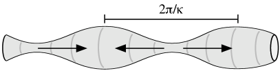
FIG. 1.: Varicose instability of a fluid cylinder, of wavelength $2\pi/\kappa$.

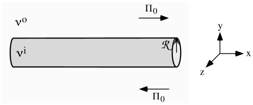
FIG. 2.: Cylindrical domain in shear flow.

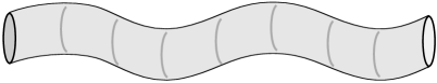
FIG. 3.: Undulation $m=1$ mode of the cylinder.

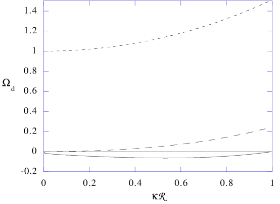
FIG. 4.: Dispersion relations in no shear, $\Omega_{0,d}$ (solid curve), $\Omega_{1,d}$ (dashed curve), and $\Omega_{2,d}$ (dotted curve).

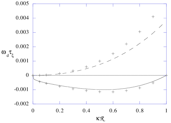
FIG. 5.: Corrections to the eigenvalues for sharp interfaces $\varpi_{0,d}$ (solid curve) and $\varpi_{1,d}$ (dashed curve) due to a finite width interface ($+$ symbols), for ${\cal R}=4\xi$.

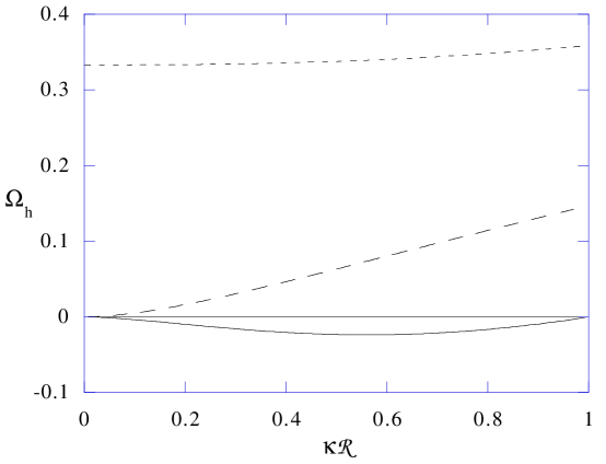
FIG. 6.: Stability eigenvalues $\Omega_{0,h}$ (solid curve), $\Omega_{1,h}$ (dashed curve), and $\Omega_{2,h}$ (dotted curve) for $\mu=1$ in the absence of shear.

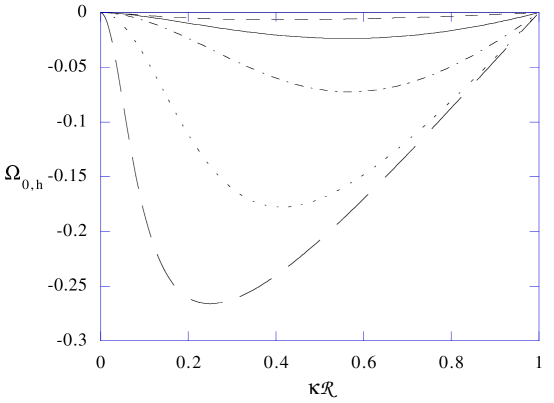
FIG. 7.: Stability eigenvalue $\Omega_{0,h}$ for $S=0$ at different $\mu$: $\mu=10$ (dashed curve), $\mu=1$ (solid curve), $\mu=.1$ (dash-dot curve), $\mu=.01$ (dotted curve), and $\mu=.001$ (long dashed curve).

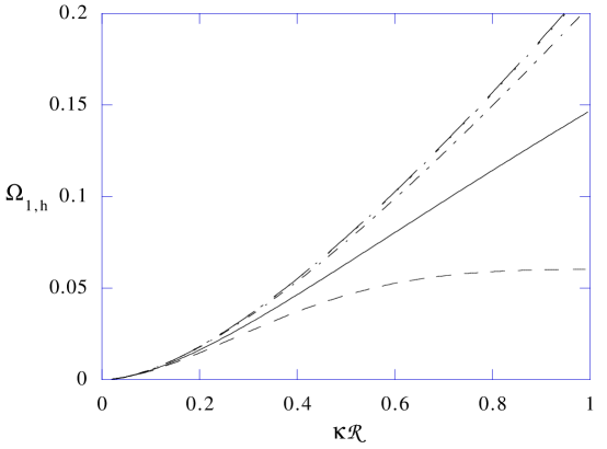
FIG. 8.: Stability eigenvalue $\Omega_{1,h}$ for $S=0$ at different $\mu$: $\mu=10$ (dashed curve), $\mu=1$ (solid curve), $\mu=.1$ (dash-dot curve), $\mu=.01$ (dotted curve), and $\mu=.001$ (long dashed curve).

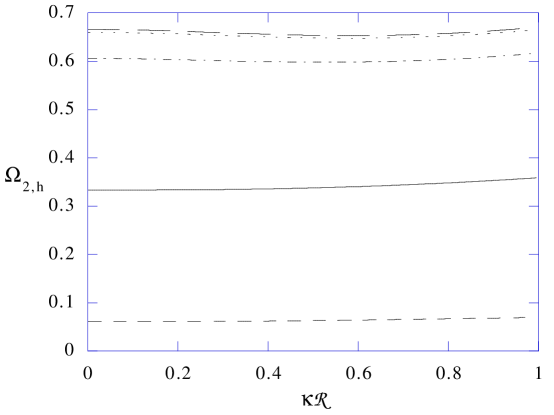
FIG. 9.: Stability eigenvalue $\Omega_{2,h}$ for $S=0$ at different $\mu$: $\mu=10$ (dashed curve), $\mu=1$ (solid curve), $\mu=.1$ (dash-dot curve), $\mu=.01$ (dotted curve), and $\mu=.001$ (long dashed curve).

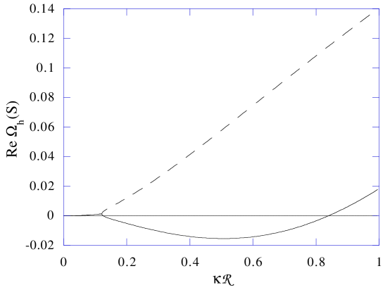
FIG. 10.: Stability eigenvalues $Re[\Omega_{0,h}(S)]$ (solid line) and $Re[\Omega_{1,h}(S)]$ (dashed line) for $\mu=1$ at $S=.1$.

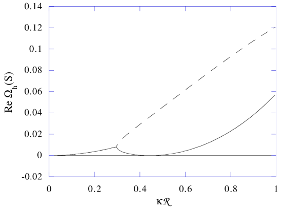
FIG. 11.: Stability eigenvalues $Re[\Omega_{0,h}(S)]$ (solid line) and $Re[\Omega_{1,h}(S)]$ (dashed line) for $\mu=1$ at the critical shear rate $S_{c}=.160$.

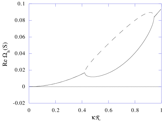
FIG. 12.: Stability eigenvalues $Re[\Omega_{0,h}(S)]$ (solid line) and $Re[\Omega_{1,h}(S)]$ (dashed line) for $\mu=1$ at $S=.18$.

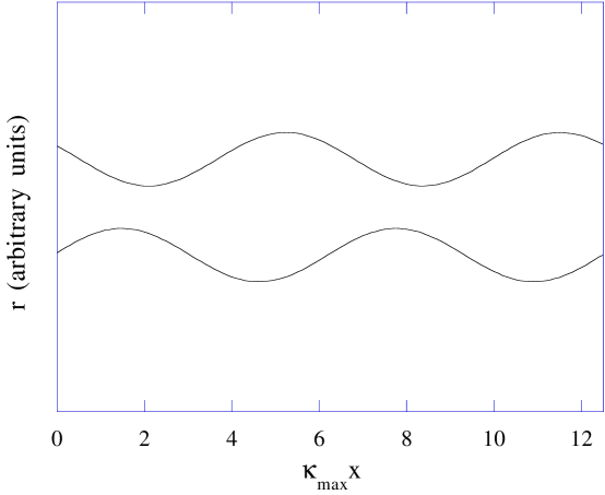
FIG. 13.: Real part of the eigenvector corresponding to $\Omega_{0,h}$ at $S=.1$, in the $\theta=0$ plane.

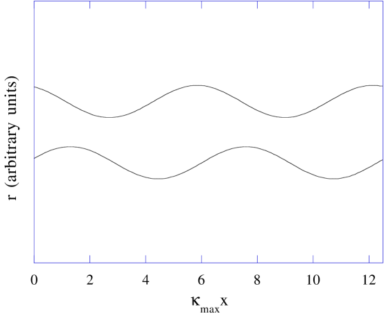
FIG. 14.: Real part of the eigenvector corresponding to $\Omega_{0,h}$ at $S=.18$, in the $\theta=0$ plane.

FIG. 15.: Stability eigenvalues $Re[\Omega_{0,h}(S)]$ (solid line) and $Re[\Omega_{1,h}(S)]$ (dashed line) for $\mu=.25$ at $S=.14$.

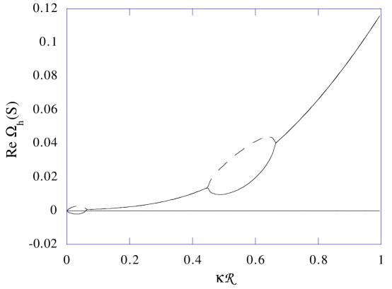
FIG. 16.: Stability eigenvalues $Re[\Omega_{0,h}(S)]$ (solid line) and $Re[\Omega_{1,h}(S)]$ (dashed line) for $\mu=.25$ at $S=.16$.

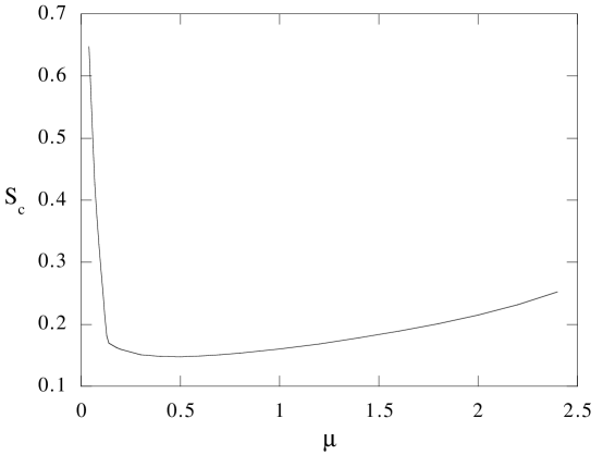
FIG. 17.: Critical shear rate as a function of viscosity ratio $\mu$.

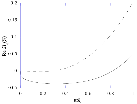
FIG. 18.: Real part of the dimensionless stability eigenvalues $\Omega_{0,d}(S)$ (solid curve) and $\Omega_{1,d}(S)$ (dashed curve) at $S^{*}=.1$ and $\mu=1$.

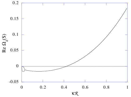
FIG. 19.: Real part of the dimensionless stability eigenvalues $\Omega_{0,d}(S)$ (solid curve) and $\Omega_{1,d}(S)$ (dashed curve) at $S^{*}=.4$ and $\mu=1$.

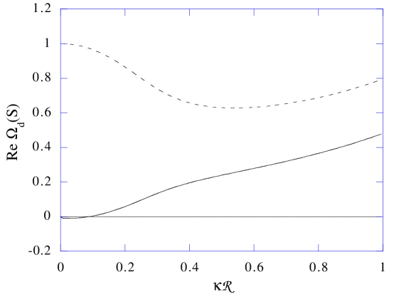
FIG. 20.: Real part of the dimensionless stability eigenvalues $\Omega_{0,d}(S)$ (solid curve), $\Omega_{1,d}(S)$ (dashed curve), and $\Omega_{2,d}(S)$ (dotted curve) at $S^{*}=2$ and $\mu=1$.

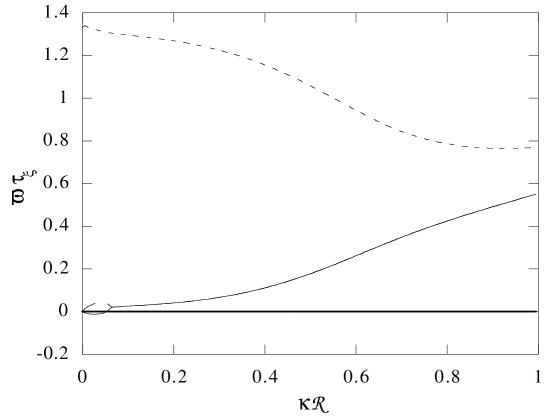
FIG. 21.: Stability eigenvalues $Re[\varpi_{0}(S)]$ (solid line), $Re[\varpi_{1}(S)]$ (dashed line), and $Re[\varpi_{2}(S)]$ (dotted line) for $\dot{\gamma}\tau_{\xi}=1.5$, $\mu=.25$, $\eta^{o}=.1$ and ${\cal R}=4\xi$.

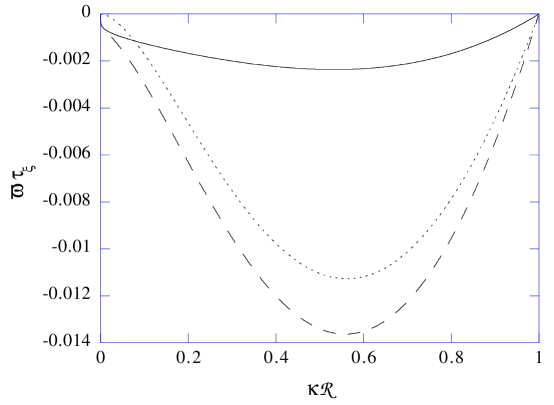
FIG. 22.: Varicose mode: $\varpi_{0,d}$ (solid line), $\varpi_{0,h}$ (dotted line), and the total $\varpi_{0}$ (dashed line) for $\eta=.7$ and ${\cal R}=3\xi$ ($S=0$).

REFERENCES

- [1] E. D. Siggia, Phys. Rev. A 20, 595 (1979).
- [2] A. Onuki, Europhys. Lett. 28, 175 (1994).
- [3] A. Onuki, Phys. Rev. A 34, 3528 (1986).
- [4] T. Hashimoto, T. Takebe, and S. Suehiro, J. Chem. Phys. 88, 5874 (1988).
- [5] K. Y. Min and W. I. Goldberg, Phys. Rev. Lett. 70, 469 (1993).
- [6] G. I. Taylor, Proc. Roy. Soc. London Ser. A 146, 501 (1934).
- [7] J. M. Rallison, Ann. Rev. Fluid Mech. 16, 46 (1984).
- [8] W. I. Goldberg and K. Y. Min, Physica A 204, 246 (1994).
- [9] T. Baumberger, F. Perrot, and D. Beysens, Physica A 174, 31 (1991).
- [10] T. Hashimoto, K. Matsuzaka, E. Moses, and A. Onuki, Phys. Rev. Lett. 74, 126 (1995).
- [11] E. K. Hobbie, S. Kim, and C. C. Han, Phys. Rev. E 54, 5909 (1996).
- [12] S. Kim, E. K. Hobbie, J.-W. Yu, and C. C. Han, Macromolecules 30, 8245 (1997).
- [13] Lord Rayleigh, Philos. Mag. 34, 145 (1892).
- [14] S. Tomotika, Proc. Roy. Soc. London A 150, 322 (1935).
- [15] A. Frischknecht, Phys. Rev. E 56, 6970 (1997).
- [16] J. S. Langer, in Solids Far from Equilibrium, Proc. 1989 Beg Rohu Summer School, edited by C. Godreche (Cambridge University Press, Cambridge, 1992).
- [17] There seems to be some debate in the literature over whether the appropriate time scale to use in dilineating weak vs. strong-shear regimes in two-phase states should be or the time scale associated with the growth/fluctuations of the domains.
- [18] E. J. Hinch and A. Acrivos, J. Fluid Mech. 98, 305 (1980).
- [19] M. J. Russo and P. H. Steen, Phys. Fluids A 1, 1926 (1989).
- [20] B. J. Lowry and P. H. Steen, J. Colloid and Interface Sci. 170, 38 (1995).
- [21] B. J. Lowry and P. H. Steen, J. Fluid Mech. 330, 189 (1997).
- [22] S. Tomotika, Proc. R. Soc. A 153, 302 (1936).
- [23] T. Mikami, R. G. Cox, and S. G. Mason, Int. J. Multiphase Flow 2, 113 (1975).
- [24] D. V. Khakhar and J. M. Ottino, Int. J. Multiphase Flow 13, 71 (1987).
- [25] J. M. H. Janssen and H. E. H. Meijer, J. Rheol. 37, 597 (1993).
- [26] P. Chaikin and T. Lubensky, Principles of Condensed Matter Physics (Cambridge University Press, Cambridge, 1995), p. 476.
- [27] P. C. Hohenberg and B. I. Halperin, Rev. Mod. Phys. 49, 435 (1977).
- [28] A. J. Bray, Advances in Physics 43, 357 (1994).
- [29] J. S. Langer, Ann. Phys. (N.Y.) 65, 53 (1971).
- [30] D. Jasnow and R. K. P. Zia, Phys. Rev. A 36, 2243 (1987).
- [31] J. Happel and H. Brenner, Low reynolds number hydrodynamics (Martinus Nijhoff, Dordrecht, The Netherlands, 1986).
- [32] H. A. Stone and M. P. Brenner, J. Fluid Mech. 318, 373 (1996).
- [33] R. Chella and J. Viñals, Phys. Rev. E 53, 3832 (1996).
- [34] T. Hashimoto (private communication); see also [10], [36], and T. Hashimoto, T. Takebe, and K. Fujioka, in Dynamics and Patterns in Complex Fluids, edited by A. Onuki and K. Kawasaki (Springer, Berlin, 1990), p. 86.
- [35] T. Takebe and T. Hashimoto, Polym. Commun. 29, 261 (1988).
- [36] T. Takebe, R. Sawaoka, and T. Hashimoto, J. Chem. Phys. 91, 4369 (1989).
- [37] D. D. Joseph and Y. Y. Renardy, Fundamentals of Two-Fluid Dynamics, Part I: Mathematical Theory and Applications (Springer-Verlag, New York, 1993), p. 25.
- [38] W. H. Press, S. A. Teukolsky, W. T. Vetterling, and B. P. Flannery, Numerical Recipes in C: The Art of Scientific Computing, 2nd ed. (Cambridge University Press, Cambridge, 1992).