A Mathematical Model for the Behavior of Individuals in a Social Field

Abstract

Related to an idea of Lewin, a mathematical model for behavioral changes under the influence of a social field is developed. The social field reflects public opinion, social norms and trends. It is not only given by external factors (the environment) but also by the interactions of individuals. Two important kinds of interaction processes are distinguished: Imitative and avoidance processes. Variations of individual behavior are taken into account by “diffusion coefficients”.
Key words: Behavioral model, field theory, diffusion model, decision theory, pair interactions, imitative and avoidance processes

A Mathematical Model for the Behavior of
Individuals in a Social Field

A Mathematical Model for the Behavior of
Individuals in a Social Field

1 Introduction

Many models have been developed for behavioral changes, but only a few are formulated in terms of mathematical relations. For example,

• game theory (von Neumann and Morgenstern, 1944), based on the concept of success of meeting strategies, is used for the description of cooperation and competition processes among individuals,

• decision theories (Domencich and McFadden, 1975, Ortúzar and Willumsen, 1990), assuming the maximization of utility, successfully model the choice behavior among several alternatives,

• diffusion models (Coleman, 1964, Bartholomew, 1967, Granovetter, 1983, Kennedy, 1983) mathematically describe the spread of behaviors or opinions, rumors, innovations, etc.

All these models are related to a more general behavioral model discussed in the following. This model is based on Boltzmann-like equations and includes spontaneous (or externally induced) behavioral changes and behavioral changes by pair interactions of individuals (sect. 2). These changes are described by transition rates. They reflect the results of mental and psychical processes, which could be simulated with the help of Osgood and Tannenbaum’s (1955) congruity principle, Heider’s (1946) balance theory or Festinger’s (1957) dissonance theory. However, it is sufficient for our model to determine the transition rates empirically (sect. 5). The ansatz used for the transition rates distinguishes imitative and avoidance processes, and assumes utility maximization by a variant of the multinomial logit model (Domencich and McFadden, 1975, Ortúzar and Willumsen, 1990) (sect. 2.1).

In section 3 a consequent mathematical formulation related to an idea of Lewin (1951) is developed, according to which the behavior of individuals is guided by a social field. This formulation is achieved by a second order Taylor approximation of the Boltzmann-like equations leading to diffusion equations. Because of their relation with the Boltzmann equation (Boltzmann, 1964) and the Fokker-Planck equation (Fokker, 1914, Planck, 1917) they will be called the Boltzmann-Fokker-Planck equations. According to these new equations the most probable behavioral change is given by a vectorial quantity that can be interpreted as social force (sect. 3.1). The social force results from external influences (the environment) as well as from individual interactions. In special cases the social force is the derivative (gradient) of a potential. This potential reflects public opinion, social norms and trends, and will be called the social field. By diffusion coefficients individual variation of the behavior (the “freedom of will”) is taken into account. In section 4 representative cases are illustrated by computer simulations.

The Boltzmann-Fokker-Planck model for the behavior of individuals under the influence of a social field shows some analogies with the physical model for the behavior of electrons in an electric field (e.g. of an atomic nucleus) (Helbing, 1992a,c). In particular, individuals and electrons influence the concrete form of the effective social, respectively, electric field. However, the behavior of electrons is governed by a different equation: the Schrödinger equation (Schrödinger, 1926, Davydov, 1976).

2 The Boltzmann-like behavioral model

Let us consider a population consisting of a great number $N\gg 1$ of individuals. Concerning a special topic of interest, these individuals show a behavior $x$ out of several possible behaviors in the set $\Omega$.

Due to “freedom of the will” one cannot expect a deterministic theory for the temporal change $d\mbox{\boldmath$x$}/dt$ of the individual behavior $\mbox{\boldmath$x$}(t)$ to be realistic. However, one can construct a model for the change of the probability distribution $P(\mbox{\boldmath$x$},t)$ of behaviors $\mbox{\boldmath$x$}(t)$ within the given population ($P(\mbox{\boldmath$x$},t)\geq 0$, $\displaystyle\sum_{x\in\Omega}P(\mbox{\boldmath$x$},t)=1$). A theory of this kind is, of course, stochastic. In order to take into account several types $a$ of behavior, we may distinguish $A$ subpopulations $a$ consisting of $N_{a}\gg 1$ individuals ($\displaystyle\sum_{a=1}^{A}N_{a}=N$). Then, the following relation holds:

$$P(\mbox{\boldmath$x$},t)=\sum_{a=1}^{A}\frac{N_{a}}{N}P_{a}(\mbox{\boldmath$x$},t)\,.$$ (1)

Our goal is now to find a suitable equation for the probability distribution $P_{a}(\mbox{\boldmath$x$},t)$ of behaviors within subpopulation $a$ ($P_{a}(\mbox{\boldmath$x$},t)\geq 0$, $\displaystyle\sum_{x\in\Omega}P_{a}(\mbox{\boldmath$x$},t)=1$). If we neglect memory effects (cf. sect. 6.1), the desired equation is of the form

$$\frac{d}{dt}P_{a}(\mbox{\boldmath$x$},t)=\mbox{inflow into $\mbox{\boldmath$x$}$}-\mbox{outflow from $\mbox{\boldmath$x$}$}\,.$$ (2)

Whereas the inflow into $x$ is given as the sum over all absolute transition rates describing changes from an arbitrary behavior $\mbox{\boldmath$x$}^{\prime}$ to $x$, the outflow from $x$ is given as the sum over all absolute transition rates describing changes from $x$ to another behavior $\mbox{\boldmath$x$}^{\prime}$. Since the absolute transition rate of changes from $x$ to $\mbox{\boldmath$x$}^{\prime}$ is the product $w^{a}(\mbox{\boldmath$x$}^{\prime}|\mbox{\boldmath$x$};t)P_{a}(\mbox{\boldmath$x$},t)$ of the relative transition rate $w^{a}(\mbox{\boldmath$x$}^{\prime}|\mbox{\boldmath$x$};t)$ for a change to behavior $\mbox{\boldmath$x$}^{\prime}$ given $x$, and the probability $P_{a}(\mbox{\boldmath$x$},t)$ of behavior $x$, we arrive at the explicit equation

$$\frac{d}{dt}P_{a}(\mbox{\boldmath$x$},t)=\sum_{x^{\prime}\in\Omega\atop(x^{\prime}\neq x)}\Big{[}w^{a}(\mbox{\boldmath$x$}|\mbox{\boldmath$x$}^{\prime};t)P_{a}(\mbox{\boldmath$x$}^{\prime},t)-w^{a}(\mbox{\boldmath$x$}^{\prime}|\mbox{\boldmath$x$};t)P_{a}(\mbox{\boldmath$x$},t)\Big{]}\,.$$ (3)

$w^{a}(\mbox{\boldmath$x$}^{\prime}|\mbox{\boldmath$x$};t)$ has the meaning of a transition probablility from $x$ to $\mbox{\boldmath$x$}^{\prime}$ per unit time and takes into account the behavioral variations between the individuals (occurring even within the same type $a$ of behavior!).

In the following we have to specify the relative transition rates $w^{a}(\mbox{\boldmath$x$}^{\prime}|\mbox{\boldmath$x$};t)$, which will turn out to be effective transition rates. If we restrict the model to spontaneous (or externally induced) behavioral changes and behavioral changes due to pair interactions, we have (Helbing, 1992a,c):

$$w^{a}(\mbox{\boldmath$x$}^{\prime}|\mbox{\boldmath$x$};t):=w_{a}(\mbox{\boldmath$x$}^{\prime}|\mbox{\boldmath$x$};t)+\sum_{b=1}^{A}\sum_{y\in\Omega}\sum_{y^{\prime}\in\Omega}N_{b}\,\widetilde{w}_{ab}(\mbox{\boldmath$x$}^{\prime},\mbox{\boldmath$y$}^{\prime}|\mbox{\boldmath$x$},\mbox{\boldmath$y$};t)P_{b}(\mbox{\boldmath$y$},t)\,.$$ (4)

$w_{a}(\mbox{\boldmath$x$}^{\prime}|\mbox{\boldmath$x$};t)$ describes the rate of spontaneous (resp. externally induced) transitions from $x$ to $\mbox{\boldmath$x$}^{\prime}$ for individuals of subpopulation $a$. $\widetilde{w}_{ab}(\mbox{\boldmath$x$}^{\prime},\mbox{\boldmath$y$}^{\prime}|\mbox{\boldmath$x$},\mbox{\boldmath$y$};t)$ is the transition rate for two individuals of types $a$ and $b$ to change their behaviors from $x$ and $y$ to $\mbox{\boldmath$x$}^{\prime}$ and $\mbox{\boldmath$y$}^{\prime}$, respectively, due to pair interactions. The total frequency of these interactions is proportional to the probability $P_{b}(\mbox{\boldmath$y$},t)$ of behavior $y$ within subpopulation $b$ and the number $N_{b}$ of individuals of type $b$. We have to sum up over $b$, $y$, and $\mbox{\boldmath$y$}^{\prime}$ since all specifications of these variables are effectively connected with transitions from $x$ to $\mbox{\boldmath$x$}^{\prime}$ of individuals of subpopulation $a$.

Inserting (4) into (3), we now obtain the socalled Boltzmann-like equations (Helbing, 1992a,c)

$$\frac{d}{dt}P_{a}(\mbox{\boldmath$x$},t) = \sum_{x^{\prime}\in\Omega}\Big{[}w_{a}(\mbox{\boldmath$x$}|\mbox{\boldmath$x$}^{\prime};t)P_{a}(\mbox{\boldmath$x$}^{\prime},t)-w_{a}(\mbox{\boldmath$x$}^{\prime}|\mbox{\boldmath$x$};t)P_{a}(\mbox{\boldmath$x$},t)\Big{]}$$

$$+ \sum_{b=1}^{A}\sum_{x^{\prime}\in\Omega}\sum_{y\in\Omega}\sum_{y^{\prime}\in\Omega}w_{ab}(\mbox{\boldmath$x$},\mbox{\boldmath$y$}^{\prime}|\mbox{\boldmath$x$}^{\prime},\mbox{\boldmath$y$};t)P_{b}(\mbox{\boldmath$y$},t)P_{a}(\mbox{\boldmath$x$}^{\prime},t)$$

$$- \sum_{b=1}^{A}\sum_{x^{\prime}\in\Omega}\sum_{y\in\Omega}\sum_{y^{\prime}\in\Omega}w_{ab}(\mbox{\boldmath$x$}^{\prime},\mbox{\boldmath$y$}^{\prime}|\mbox{\boldmath$x$},\mbox{\boldmath$y$};t)P_{b}(\mbox{\boldmath$y$},t)P_{a}(\mbox{\boldmath$x$},t)$$ (5b)

with

$$w_{ab}(\mbox{\boldmath$x$}^{\prime},\mbox{\boldmath$y$}^{\prime}|\mbox{\boldmath$x$},\mbox{\boldmath$y$};t):=N_{b}\,\widetilde{w}_{ab}(\mbox{\boldmath$x$}^{\prime},\mbox{\boldmath$y$}^{\prime}|\mbox{\boldmath$x$},\mbox{\boldmath$y$};t)\,.$$ (6)

Obviously, (2b) depends nonlinearly (quadratically) on the probability distributions $P_{a}(\mbox{\boldmath$x$},t)$ (resp. $P_{b}(\mbox{\boldmath$y$},t)$) which is due to the pair interactions.

The Boltzmann-like equations originally had been developed for the description of the kinetics of gases (Boltzmann, 1964). However, they have also been applied to attitude formation (Helbing, 1992b,c) and the avoidance behavior of pedestrians (Helbing, 1992c,d).

It is possible to generalize the model to simultaneous interactions of an arbitrary number of individuals (i.e., higher order interactions) (Helbing, 1992a,c). However, in most cases behavioral changes are dominated by pair interactions (dyadic interactions). Many of the phenomena occurring in social interaction processes can already be understood in terms of pair interactions.

2.1 The form of the transition rates

For models of behavioral changes the following special form of the effective transition rates (4) has been found to be suitable (Helbing, 1992b,c,e):

$$w^{a}(\mbox{\boldmath$x$}^{\prime}|\mbox{\boldmath$x$};t):=\nu_{a}(t)R_{a}(\mbox{\boldmath$x$}^{\prime}|\mbox{\boldmath$x$};t)+\sum_{b=1}^{A}\nu_{ab}(t)\Big{[}f_{ab}^{1}(t)P_{b}(\mbox{\boldmath$x$}^{\prime},t)+f_{ab}^{2}(t)P_{b}(\mbox{\boldmath$x$},t)\Big{]}R^{a}(\mbox{\boldmath$x$}^{\prime}|\mbox{\boldmath$x$};t)\,.$$ (7)

Here,

• $\nu_{a}(t)$ is a measure of the rate of spontaneous (or externally induced) behavioral changes within subpopulation $a$.

• $R_{a}(\mbox{\boldmath$x$}^{\prime}|\mbox{\boldmath$x$};t)$ [resp. $R^{a}(\mbox{\boldmath$x$}^{\prime}|\mbox{\boldmath$x$};t)$] is the readiness of an individual of subpopulation $a$ to change behavior from $x$ to $\mbox{\boldmath$x$}^{\prime}$ spontaneously [resp. in pair interactions].

• $\nu_{ab}(t)\equiv N_{b}\,\widetilde{\nu}_{ab}(t)$ is the interaction rate of an individual of subpopulation $a$ with individuals of subpopulation $b$.

• $f_{ab}^{1}(t)$ is a measure for the frequency of imitative processes

  $$\mbox{\boldmath$x$}^{\prime},\mbox{\boldmath$x$}^{\prime}\longleftarrow\mbox{\boldmath$x$},\mbox{\boldmath$x$}^{\prime}\qquad(\mbox{\boldmath$x$}\neq\mbox{\boldmath$x$}^{\prime})\,,$$ (8)

  where an individual of subpopulation $a$ takes over the behavior $\mbox{\boldmath$x$}^{\prime}$ of an individual of subpopulation $b$. The total frequency of imitative processes is proportional to the probablility $P_{b}(\mbox{\boldmath$x$}^{\prime},t)$ of behavior $\mbox{\boldmath$x$}^{\prime}$ within subpopulation $b$.

• $f_{ab}^{2}(t)$ is a measure for the frequency of avoidance processes

  $$\mbox{\boldmath$x$}^{\prime},\mbox{\boldmath$x$}\longleftarrow\mbox{\boldmath$x$},\mbox{\boldmath$x$}\qquad(\mbox{\boldmath$x$}\neq\mbox{\boldmath$x$}^{\prime})\,,$$ (9)

  where an individual of subpopulation $a$ changes the behavior $x$ to another behavior $\mbox{\boldmath$x$}^{\prime}$ if meeting an individual of subpopulation $b$ with the same behavior (defiant behavior, snob effect). The total frequency of avoidance processes is proportional to the probablility $P_{b}(\mbox{\boldmath$x$},t)$ of behavior $x$ within subpopulation $b$.

A more detailled discussion of the different kinds of interaction processes and of ansatz (7) is given in publications of Helbing (1992b,c,e).

For $R^{a}(\mbox{\boldmath$x$}^{\prime}|\mbox{\boldmath$x$};t)$ we take the quite general form

$$R^{a}(\mbox{\boldmath$x$}^{\prime}|\mbox{\boldmath$x$};t)=\frac{\mbox{e}^{U^{a}(x^{\prime},t)-U^{a}(x,t)}}{D_{a}(\mbox{\boldmath$x$}^{\prime},\mbox{\boldmath$x$};t)}$$ (10a)

with

$$D_{a}(\mbox{\boldmath$x$}^{\prime},\mbox{\boldmath$x$};t)=D_{a}(\mbox{\boldmath$x$},\mbox{\boldmath$x$}^{\prime};t)>0$$

(cf. Weidlich and Haag, 1988, Helbing, 1992c). Then, the readiness $R^{a}(\mbox{\boldmath$x$}^{\prime}|\mbox{\boldmath$x$};t)$ for an individual of subpopulation $a$ to change behavior from $x$ to $\mbox{\boldmath$x$}^{\prime}$ will be greater,

• the greater the difference in the utilities $U^{a}(.,t)$ of behaviors $\mbox{\boldmath$x$}^{\prime}$ and $x$,

• the smaller the incompatibility (“distance”) $D_{a}(\mbox{\boldmath$x$}^{\prime},\mbox{\boldmath$x$};t)$ between the behaviors $x$ and $\mbox{\boldmath$x$}^{\prime}$.

Similar to (10a) we use

$$R_{a}(\mbox{\boldmath$x$}^{\prime}|\mbox{\boldmath$x$};t)=\frac{\mbox{e}^{U_{a}(x^{\prime},t)-U_{a}(x,t)}}{D_{a}(\mbox{\boldmath$x$}^{\prime},\mbox{\boldmath$x$};t)}\,,$$ (10b)

and, therefore, allow the utility function $U_{a}(\mbox{\boldmath$x$},t)$ for spontaneous (or externally induced) behavioral changes to differ from the utility function $U^{a}(\mbox{\boldmath$x$},t)$ for behavioral changes in pair interactions. Ansatz (2.1) is related to the multinomial logit model (Domencich and McFadden, 1975, Ortúzar and Willumsen, 1990). It assumes utility maximization with incomplete information about the exact utility of a behavioral change from $x$ to $\mbox{\boldmath$x$}^{\prime}$, which is, therefore, estimated and stochastically varying (cf. Helbing, 1992c).

Computer simulations of the Boltzmann-like equations (3), (7), (2.1) are discussed and illustrated in Helbing (1992b,c,e) (cf. also sect. 4).

2.2 Special fields of application in the social sciences

The Boltzmann-like equations (3), (7) include a variety of special cases, which have become very important in the social sciences:

• The logistic equation (Pearl, 1924, Verhulst, 1845) describes limited growth processes. Let us consider the situation of two behaviors $\mbox{\boldmath$x$}\equiv x\in\{1,2\}$ (i.e., $P_{a}(1,t)=1-P_{a}(2,t)$) and one subpopulation ($A=1$). $x=2$ may, for example, have the meaning to apply a certain strategy, and $x=1$ not to do so. If only imitative processes

  $$2,2\longleftarrow 1,2$$ (11)

  and processes of spontaneous replacement

  $$1\longleftarrow 2$$ (12)

  are considered, one arrives at the logistic equation

  $$\frac{d}{dt}P_{1}(2,t) = -\nu_{1}(t)R_{1}(1|2;t)P_{1}(2,t)+\nu_{11}(t)f_{11}^{1}(t)R^{1}(2|1;t)\Big{(}1-P_{1}(2,t)\Big{)}P_{1}(2,t)$$ (13)

  $$\equiv A(t)P_{1}(2,t)\Big{(}B(t)-P_{1}(2,t)\Big{)}\,.$$

• The gravity model (Zipf, 1946, Ravenstein, 1876) describes processes of exchange between different places $x$. Its dynamical version results for $R_{a}(\mbox{\boldmath$x$}^{\prime}|\mbox{\boldmath$x$};t)\equiv 0$, $f_{ab}^{1}(t)\equiv 1$, $f_{ab}^{2}(t)\equiv 0$, and $A=1$:

  $$\frac{d}{dt}P(\mbox{\boldmath$x$},t)=\nu(t)\sum_{x^{\prime}\in\Omega}\left[\frac{\mbox{e}^{U(x,t)-U(x^{\prime},t)}}{D(\mbox{\boldmath$x$},\mbox{\boldmath$x$}^{\prime})}-\frac{\mbox{e}^{U(x^{\prime},t)-U(x,t)}}{D(\mbox{\boldmath$x$}^{\prime},\mbox{\boldmath$x$})}\right]P(\mbox{\boldmath$x$},t)P(\mbox{\boldmath$x$}^{\prime},t)\,.$$ (14)

  Here, we have dropped the index $a$ because of $a=1$. $P(\mbox{\boldmath$x$},t)$ is the probability of being at place $x$. The absolute rate of exchange from $x$ to $\mbox{\boldmath$x$}^{\prime}$ is proportional to the probabilities $P(\mbox{\boldmath$x$},t)$ and $P(\mbox{\boldmath$x$}^{\prime},t)$ at the places $x$ and $\mbox{\boldmath$x$}^{\prime}$. $D(\mbox{\boldmath$x$},\mbox{\boldmath$x$}^{\prime})$ is often chosen as a function of the metric distance $\|\mbox{\boldmath$x$}-\mbox{\boldmath$x$}^{\prime}\|$ between $x$ and $\mbox{\boldmath$x$}^{\prime}$: $D(\mbox{\boldmath$x$},\mbox{\boldmath$x$}^{\prime})\equiv D(\|\mbox{\boldmath$x$}-\mbox{\boldmath$x$}^{\prime}\|)$.

• The behavioral model of Weidlich and Haag (1983, 1988, Weidlich, 1991, 1994) is based on spontaneous transitions. We obtain this model for $f_{ab}^{1}(t)\equiv 0\equiv f_{ab}^{2}(t)$ and

  $$U_{a}(\mbox{\boldmath$x$},t):=\delta_{a}(\mbox{\boldmath$x$},t)+\sum_{b=1}^{A}\kappa_{ab}\,P_{b}(\mbox{\boldmath$x$},t)\,.$$ (15)

  Because of the dependence of the utilities $U_{a}(\mbox{\boldmath$x$},t)$ on the behavioral distributions $P_{b}(\mbox{\boldmath$x$},t)$ the model assumes indirect interactions, which are, for example, mediated by the newspapers, TV or radio. $\delta_{a}(\mbox{\boldmath$x$},t)$ is the preference of subpopulation $a$ for behavior $x$. $\kappa_{ab}$ are coupling parameters describing the influence of the behaviorial distribution within subpopulation $b$ on the behavior of subpoplation $a$. For $\kappa_{ab}>0$, $\kappa_{ab}$ reflects the social pressure of behavioral majorities.

• The game dynamical equations (Hofbauer and Sigmund, 1988, Schuster et. al., 1981, Helbing, 1992c,e, 1993) result for $f_{ab}^{1}(t)\equiv\delta_{ab}$, $f_{ab}^{2}(t)\equiv 0$, and

  $$R^{a}(\mbox{\boldmath$x$}^{\prime}|\mbox{\boldmath$x$};t):=\max\Big{(}E_{a}(\mbox{\boldmath$x$}^{\prime},t)-E_{a}(\mbox{\boldmath$x$},t),0\Big{)}\,,$$ (16)

  where

  $$\delta_{ab}:=\left\{\begin{array}[]{ll}1&\mbox{if }a=b\\ 0&\mbox{if }a\neq b\end{array}\right.\qquad\mbox{and}\qquad\max(x,y):=\left\{\begin{array}[]{ll}x&\mbox{if }x\geq y\\ y&\mbox{if }y>x\,.\end{array}\right.$$ (17)

  For a detailled interpretation of these relations see Helbing (1992c,e).

  The explicit form of the game dynamical equations is

  $$\frac{d}{dt}P_{a}(\mbox{\boldmath$x$},t) = \sum_{x^{\prime}\in\Omega}\Big{[}w_{a}(\mbox{\boldmath$x$}|\mbox{\boldmath$x$}^{\prime};t)P_{a}(\mbox{\boldmath$x$}^{\prime},t)-w_{a}(\mbox{\boldmath$x$}^{\prime}|\mbox{\boldmath$x$};t)P_{a}(\mbox{\boldmath$x$},t)\Big{]}$$ (18a)

  $$+ \nu_{aa}(t)P_{a}(\mbox{\boldmath$x$},t)\Big{[}E_{a}(\mbox{\boldmath$x$},t)-\langle E_{a}\rangle\Big{]}\,.$$ (18b)

  Whereas (• ‣ 2.2a) again describes spontaneous behavioral changes (“mutations”, innovations), (• ‣ 2.2b) reflects competition processes leading to a “selection” of behaviors with a success $E_{a}(\mbox{\boldmath$x$},t)$ that exceeds the average success

  $$\langle E_{a}\rangle:=\sum_{x^{\prime}\in\Omega}E_{a}(\mbox{\boldmath$x$}^{\prime},t)P_{a}(\mbox{\boldmath$x$}^{\prime},t)\,.$$ (19)

  The success $E_{a}(\mbox{\boldmath$x$},t)$ is connected with the socalled payoff matrices $\underline{A}_{ab}\equiv\Big{(}A_{ab}(\mbox{\boldmath$x$},\mbox{\boldmath$y$})\Big{)}$ by

  $$E_{a}(\mbox{\boldmath$x$},t):=A_{a}(\mbox{\boldmath$x$})+\sum_{b=1}^{A}\sum_{y\in\Omega}A_{ab}(\mbox{\boldmath$x$},\mbox{\boldmath$y$})P_{b}(\mbox{\boldmath$y$},t)$$ (20)

  (Helbing, 1992c,e). $A_{a}(\mbox{\boldmath$x$})$ means the success of behavior $x$ with respect to the environment.

  Since the game dynamical equations (• ‣ 2.2) agree with the selection mutation equations (Hofbauer and Sigmund, 1988) they are not only a powerful tool in social sciences and economy (Axelrod, 1984, von Neumann and Morgenstern, 1944, Schuster et. al., 1981, Helbing, 1992c,e, 1993), but also in evolutionary biology (Fisher, 1930, Eigen, 1971, Eigen and Schuster, 1979, Feistel and Ebeling, 1989).

3 The Boltzmann-Fokker-Planck equations

We shall now assume the set $\Omega$ of possible behaviors forms a continuous space. The $n$ dimensions of this space correspond to different characteristic aspects of the considered behaviors. In the continuous formulation, the sums in (3), (4) have to be replaced by integrals:

$$\frac{d}{dt}P_{a}(\mbox{\boldmath$x$},t)=\int\limits_{\Omega}d^{n}x^{\prime}\,\Big{[}w^{a}(\mbox{\boldmath$x$}|\mbox{\boldmath$x$}^{\prime};t)P_{a}(\mbox{\boldmath$x$}^{\prime},t)-w^{a}(\mbox{\boldmath$x$}^{\prime}|\mbox{\boldmath$x$};t)P_{a}(\mbox{\boldmath$x$},t)\Big{]}\,,$$ (21a)

$$w^{a}(\mbox{\boldmath$x$}^{\prime}|\mbox{\boldmath$x$};t):=w_{a}(\mbox{\boldmath$x$}^{\prime}|\mbox{\boldmath$x$};t)+\sum_{b=1}^{A}\int\limits_{\Omega}d^{n}y\int\limits_{\Omega}d^{n}y^{\prime}\,N_{b}\,\widetilde{w}_{ab}(\mbox{\boldmath$x$}^{\prime},\mbox{\boldmath$y$}^{\prime}|\mbox{\boldmath$x$},\mbox{\boldmath$y$};t)P_{b}(\mbox{\boldmath$y$},t)\,.$$ (21b)

A reformulation of the Boltzmann-like equations (3) via a second order Taylor approximation (Kramers-Moyal expansion (Kramers, 1940, Moyal, 1949)) leads to diffusion equations (Helbing, 1992a,c):

$$\frac{\partial}{\partial t}P_{a}(\mbox{\boldmath$x$},t)=-\sum_{i=1}^{n}\frac{\partial}{\partial x_{i}}\Big{[}K_{ai}(\mbox{\boldmath$x$},t)P_{a}(\mbox{\boldmath$x$},t)\Big{]}+\frac{1}{2}\sum_{i,j=1}^{n}\frac{\partial}{\partial x_{i}}\frac{\partial}{\partial x_{j}}\Big{[}Q_{aij}(\mbox{\boldmath$x$},t)P_{a}(\mbox{\boldmath$x$},t)\Big{]}$$ (22a)

with the effective drift coefficients

$$K_{ai}(\mbox{\boldmath$x$},t):=\int\limits_{\Omega}\!d^{n}x^{\prime}\,(x^{\prime}_{i}-x_{i})w^{a}(\mbox{\boldmath$x$}^{\prime}|\mbox{\boldmath$x$};t)$$ (22b)

and the effective diffusion coefficients

$$Q_{aij}(\mbox{\boldmath$x$},t):=\displaystyle\int\limits_{\Omega}\!d^{n}x^{\prime}\,(x^{\prime}_{i}-x_{i})(x^{\prime}_{j}-x_{j})w^{a}(\mbox{\boldmath$x$}^{\prime}|\mbox{\boldmath$x$};t)\,.$$ (22c)

Because of their relation with the Boltzmann equation (Boltzmann, 1964) and the Fokker-Planck equation (Fokker, 1914, Planck, 1917) equations (21b) will be called the Boltzmann-Fokker-Planck equations in the following (cf. Helbing 1992a,c). In the Boltzmann-Fokker-Planck equations the drift coefficients $K_{ai}(\mbox{\boldmath$x$},t)$ govern the systematic change (“drift”, motion) of the distribution $P_{a}(\mbox{\boldmath$x$},t)$, whereas the diffusion coefficients $Q_{aij}(\mbox{\boldmath$x$},t)$ describe the spread of the distribution $P_{a}(\mbox{\boldmath$x$},t)$ due to fluctuations resulting from the individual variation of behavioral changes.

For ansatz (7), the effective drift and diffusion coefficients can be split into contributions due to spontaneous (or externally induced) transitions ($k=0$), imitative processes ($k=1$), and avoidance processes ($k=2$):

$$K_{ai}(\mbox{\boldmath$x$},t)=\sum_{k=0}^{2}K_{ai}^{k}(\mbox{\boldmath$x$},t)\,,\qquad Q_{aij}(\mbox{\boldmath$x$},t)=\sum_{k=0}^{2}Q_{aij}^{k}(\mbox{\boldmath$x$},t)\,,$$ (23a)

where

$$K_{ai}^{0}(\mbox{\boldmath$x$},t) := \nu_{a}(t)\int\!d^{n}x^{\prime}\,(x^{\prime}_{i}-x_{i})R_{a}(\mbox{\boldmath$x$}^{\prime}|\mbox{\boldmath$x$};t)\,,$$

$$K_{ai}^{1}(\mbox{\boldmath$x$},t) := \sum_{b=1}^{A}\nu_{ab}(t)f_{ab}^{1}(t)\int\!d^{n}x^{\prime}\,(x^{\prime}_{i}-x_{i})R^{a}(\mbox{\boldmath$x$}^{\prime}|\mbox{\boldmath$x$};t)P_{b}(\mbox{\boldmath$x$}^{\prime},t)\,,$$

$$K_{ai}^{2}(\mbox{\boldmath$x$},t) := \sum_{b=1}^{A}\nu_{ab}(t)f_{ab}^{2}(t)\int\!d^{n}x^{\prime}\,(x^{\prime}_{i}-x_{i})R^{a}(\mbox{\boldmath$x$}^{\prime}|\mbox{\boldmath$x$};t)P_{b}(\mbox{\boldmath$x$},t)$$ (23b)

and

$$Q_{aij}^{0}(\mbox{\boldmath$x$},t) := \nu_{a}(t)\int\!d^{n}x^{\prime}\,(x^{\prime}_{i}-x_{i})(x^{\prime}_{j}-x_{j})R_{a}(\mbox{\boldmath$x$}^{\prime}|\mbox{\boldmath$x$};t)\,,$$

$$Q_{aij}^{1}(\mbox{\boldmath$x$},t) := \sum_{b=1}^{A}\nu_{ab}(t)f_{ab}^{1}(t)\int\!d^{n}x^{\prime}\,(x^{\prime}_{i}-x_{i})(x^{\prime}_{j}-x_{j})R^{a}(\mbox{\boldmath$x$}^{\prime}|\mbox{\boldmath$x$};t)P_{b}(\mbox{\boldmath$x$}^{\prime},t)\,,$$

$$Q_{aij}^{2}(\mbox{\boldmath$x$},t) := \sum_{b=1}^{A}\nu_{ab}(t)f_{ab}^{2}(t)\int\!d^{n}x^{\prime}\,(x^{\prime}_{i}-x_{i})(x^{\prime}_{j}-x_{j})R^{a}(\mbox{\boldmath$x$}^{\prime}|\mbox{\boldmath$x$};t)P_{b}(\mbox{\boldmath$x$},t)\,.$$ (23c)

The behavioral changes induced by the environment are included in $K_{ai}^{0}(\mbox{\boldmath$x$},t)$ and $Q_{aij}^{0}(\mbox{\boldmath$x$},t)$.

3.1 Social force and social field

The Boltzmann-Fokker-Planck equations (21b) are equivalent to the stochastic equations (Langevin equations, 1908)

$$\frac{dx_{i}}{dt}=F_{ai}(\mbox{\boldmath$x$},t)+\sum_{j=1}^{n}G_{aij}(\mbox{\boldmath$x$},t)\xi_{j}(t)$$ (24a)

with

$$K_{ai}(\mbox{\boldmath$x$},t)=F_{ai}(\mbox{\boldmath$x$},t)+\frac{1}{2}\sum_{j,k=1}^{n}\left[\frac{\partial}{\partial x_{k}}G_{aij}(\mbox{\boldmath$x$},t)\right]G_{ajk}(\mbox{\boldmath$x$},t)$$ (24b)

and

$$Q_{aij}(\mbox{\boldmath$x$},t)=\sum_{k=1}^{n}G_{aik}(\mbox{\boldmath$x$},t)G_{akj}(\mbox{\boldmath$x$},t)$$ (24c)

(cf. Stratonovich, 1963, Helbing, 1992c). For an individual of subpopulation $a$ the vector $\mbox{\boldmath$\zeta$}_{a}(\mbox{\boldmath$x$},t)$ with the components

$$\zeta_{ai}(\mbox{\boldmath$x$},t)=\sum_{j=1}^{n}G_{aij}(\mbox{\boldmath$x$},t)\xi_{j}(t)$$ (25)

describes the contribution to the change of behavior $x$ that is caused by behavioral fluctuations $\mbox{\boldmath$\xi$}(t)$ (which are assumed to be delta-correlated and Gaussian (Helbing, 1992c)). Since the diffusion coefficients $Q_{aij}(\mbox{\boldmath$x$},t)$ and the coefficients $G_{aij}(\mbox{\boldmath$x$},t)$ are usually small quantities, we have $F_{ai}(\mbox{\boldmath$x$},t)\approx K_{ai}(\mbox{\boldmath$x$},t)$ (cf. (24b)), and (24a) can be put into the form

$$\frac{d\mbox{\boldmath$x$}}{dt}\approx\mbox{\boldmath$K$}_{a}(\mbox{\boldmath$x$},t)+\mbox{\em fluctuations.}$$ (26)

Whereas the fluctuation term describes individual behavioral variations, the vectorial quantity

$$\mbox{\boldmath$K$}_{a}(\mbox{\boldmath$x$},t):=\left(\begin{array}[]{c}K_{a1}(\mbox{\boldmath$x$},t)\\ \vdots\\ K_{an}(\mbox{\boldmath$x$},t)\end{array}\right)$$ (27)

drives the systematic change of the behavior $\mbox{\boldmath$x$}(t)$ of individuals of subpopulation $a$. Therefore, it is justified to denote $\mbox{\boldmath$K$}_{a}(\mbox{\boldmath$x$},t)$ as social force acting on individuals of subpopulation $a$. With that we have attained a very intuitive formulation of social processes, according to which behavioral changes are caused by social forces.

On the one hand, social forces influence the behavior of the individuals, but on the other hand, due to interactions, the behavior of the individuals also influences the social forces via the behavioral distributions $P_{a}(\mbox{\boldmath$x$},t)$ (cf. (3b), (22b)). That means, $K_{a}(\mbox{\boldmath$x$},t)$ is a function of the social processes within the given population.

Under the integrability conditions

$$\frac{\partial}{\partial x_{j}}K_{ai}(\mbox{\boldmath$x$},t)=\frac{\partial}{\partial x_{i}}K_{aj}(\mbox{\boldmath$x$},t)\qquad\mbox{for all }i,j$$ (28)

there exists a time-dependent potential

$$V_{a}(\mbox{\boldmath$x$},t):=-\int\limits^{x}d\mbox{\boldmath$x$}^{\prime}\cdot\mbox{\boldmath$K$}_{a}(\mbox{\boldmath$x$}^{\prime},t)\equiv-\sum_{i=1}^{n}\int\limits^{x}dx^{\prime}_{i}\,K_{ai}(\mbox{\boldmath$x$}^{\prime},t)\,,$$ (29)

so that the social force is given by its derivative (by its gradient $\nabla$):

$$\mbox{\boldmath$K$}_{a}(\mbox{\boldmath$x$},t)=-\nabla V_{a}(\mbox{\boldmath$x$},t)\,,\qquad\mbox{i.e.,}\qquad K_{ai}(\mbox{\boldmath$x$},t)=-\frac{\partial}{\partial x_{i}}V_{a}(\mbox{\boldmath$x$},t)\,.$$ (30)

The potential $V_{a}(\mbox{\boldmath$x$},t)$ can be understood as social field. It reflects the social influences and interactions relevant for behavioral changes: the public opinion, trends, social norms, etc.

3.2 Discussion of the concept of force

Clearly, the social force is not a force obeying the Newtonian (1687) laws of mechanics (cf. Greenwood, 1988). Instead, the social force $\mbox{\boldmath$K$}_{a}(\mbox{\boldmath$x$},t)$ is a vectorial quantity with the following properties:

• $\mbox{\boldmath$K$}_{a}(\mbox{\boldmath$x$},t)$ drives the temporal change $d\mbox{\boldmath$x$}/dt$ of another vectorial quantity: the behavior $\mbox{\boldmath$x$}(t)$ of an individual of subpopulation $a$.

• The component

  $$\mbox{\boldmath$K$}_{ab}(\mbox{\boldmath$x$},t):=\nu_{ab}(t)\int\limits_{\Omega}d^{n}x^{\prime}\,(\mbox{\boldmath$x$}^{\prime}-\mbox{\boldmath$x$})\Big{[}f_{ab}^{1}(t)P_{b}(\mbox{\boldmath$x$}^{\prime},t)+f_{ab}^{2}(t)P_{b}(\mbox{\boldmath$x$},t)\Big{]}R^{a}(\mbox{\boldmath$x$}^{\prime}|\mbox{\boldmath$x$};t)$$ (31)

  of the social force $\mbox{\boldmath$K$}_{a}(\mbox{\boldmath$x$},t)$ describes the reaction of subpopulation $a$ on the behavioral distribution within subpopulation $b$ and usually differs from $\mbox{\boldmath$K$}_{ba}(\mbox{\boldmath$x$},t)$, which describes the influence of subpopulation $a$ on subpopulation $b$.

• Neglecting fluctuations, the behavior $\mbox{\boldmath$x$}(t)$ does not change if $\mbox{\boldmath$K$}_{a}(\mbox{\boldmath$x$},t)$ vanishes. $\mbox{\boldmath$K$}_{a}(\mbox{\boldmath$x$},t)=\mbox{\bf 0}$ corresponds to an extremum of the social field $V_{a}(\mbox{\boldmath$x$},t)$, because it means

  $$\nabla V_{a}(\mbox{\boldmath$x$},t)=\mbox{\bf 0}\,,\qquad\mbox{i.e.,}\qquad\frac{\partial}{\partial x_{i}}V_{a}(\mbox{\boldmath$x$},t)=0\quad\mbox{for all }i\in\{1,\dots,n\}\,.$$ (32)

We will now compare our results with Lewin’s (1951) social field theory. From social psychology it is well-known that the behavior of an individual is determined by the totality of environmental influences and his or her personality. Inspired by electro-magnetic field theory, social field theory claims that environmental influences can be considered as a dynamical force field, which should be mathematically representable. A temporal change of this field will evoke a psychical tension which, then, induces a (behavioral) compensation.

In the following it will turn out that our model allows a fully mathematical specification of the field theoretical ideas, which was still to be found:

• Let us assume that an individual’s objective is to behave in an optimal way with respect to the social field $V_{a}(\mbox{\boldmath$x$},t)$, that means, he or she tends to a behavior corresponding to a minimum of the social field.

• If the behavior $x$ does not agree with a minimum of the social field $V_{a}(\mbox{\boldmath$x$},t)$ this evokes a force

  $$\mbox{\boldmath$K$}_{a}(\mbox{\boldmath$x$},t)=-\nabla V_{a}(\mbox{\boldmath$x$},t)$$ (33)

  that is given by the gradient of the social field $V_{a}(\mbox{\boldmath$x$},t)$ (pulling into the direction of steepest descent of $V_{a}(\mbox{\boldmath$x$},t)$). The force $\mbox{\boldmath$K$}_{a}(\mbox{\boldmath$x$},t)$ plays the role of the psychical tension. It induces a behavioral change according to

  $$\frac{d\mbox{\boldmath$x$}}{dt}\approx\mbox{\boldmath$K$}_{a}(\mbox{\boldmath$x$},t)\,.$$ (34)

• The behavioral change $d\mbox{\boldmath$x$}/dt$ drives the behavior $\mbox{\boldmath$x$}(t)$ towards a minimum $\mbox{\boldmath$x$}_{a}^{*}$ of the social field $V_{a}(\mbox{\boldmath$x$},t)$. When the minimum $\mbox{\boldmath$x$}_{a}^{*}$ is reached, then

  $$\nabla V_{a}(\mbox{\boldmath$x$},t)=\mbox{\bf 0}$$ (35)

  holds and, therefore, $\mbox{\boldmath$K$}_{a}(\mbox{\boldmath$x$},t)=\mbox{\bf 0}$. As a consequence, the psychical tension vanishes, that means, it is compensated by the previous behavioral changes.

  When the psychical tension $\mbox{\boldmath$K$}_{a}(\mbox{\boldmath$x$},t)$ vanishes then, except for fluctuations, no behavioral changes take place—in accordance with (34). The individual has reached an equilibrium within the social field, then.

• Note, that the social fields $V_{a}(\mbox{\boldmath$x$},t)$ of different subpopulations $a$ usually have different minima $\mbox{\boldmath$x$}_{a}^{*}$. This means that individuals of different types $a$ of behavior will normally feel different psychical tensions $\mbox{\boldmath$K$}_{a}(\mbox{\boldmath$x$},t)$. In other words, index $a$ distinguishes different personalities.

4 Computer simulations

The Boltzmann-Fokker-Planck equations are able to describe a broad spectrum of social phenomena. In the following, some of the results shall be illustrated by computer simulations. We shall examine the case of $A=2$ subpopulations, and a situation for which the interesting aspect of the individual behavior can be described by a certain position $x$ on a one-dimensional continuous scale (i.e., $n=1$, $\mbox{\boldmath$x$}\equiv x$). A concrete example for this situation would be the case of opinion formation. Here, conservative and progressive thinking individuals could be distinguished by different subpopulations. The position $x$ would describe the grade of approval or disapproval with respect to a certain political option (for example, SDI, power stations, Golf war, etc.).

In the one-dimensional case, the integrability conditions (28) are automatically fulfilled, and the social field

$$V_{a}(x,t)=-\int\limits_{x_{0}}^{x}dx^{\prime}\,K_{a}(x^{\prime},t)-c_{a}(t)$$ (36)

is well-defined. The parameter $c_{a}(t)$ can be chosen arbitrarily. We will take for $c_{a}(t)$ the value that shifts the absolute minimum of $V_{a}(x,t)$ to zero, that means,

$$c_{a}(t):=\min_{x}\left(-\int\limits_{x_{0}}^{x}dx^{\prime}\,K_{a}(x^{\prime},t)\right)\,.$$ (37)

• Since we will restrict the simulations to the case of imitative or avoidance processes, the shape of the social field $V_{a}(x,t)$ changes with time only due to changes of the probability distributions $P_{a}(x,t)$ (cf. (3)), that means, due to behavioral changes of the individuals (see figures 1 to 6).

In the one-dimensional case one can find the formal stationary solution

$$P_{a}(x)=P_{a}(x_{0})\frac{Q_{a}(x_{0})}{Q_{a}(x)}\exp\left(2\int\limits_{x_{0}}^{x}dx^{\prime}\,\frac{K_{a}(x^{\prime})}{Q_{a}(x^{\prime})}\right)\,,$$ (38)

which we expect to be approached in the limit of large times $t\rightarrow\infty$. Due to the dependence of $K_{a}(x)$ and $Q_{a}(x)$ on $P_{a}(x)$, equations (38) are only implicit equations. However, from (38) we can derive the following conclusions:

• If the diffusion coefficients are constant ($Q_{a}(x)\equiv Q_{a}$), (38) simplifies to

  $$P_{a}(x)=P_{a}(x_{0})\exp\left(-\frac{2}{Q_{a}}\Big{[}V_{a}(x)+c_{a}\Big{]}\right)\,,$$ (39)

  that means, the stationary solution $P_{a}(x)$ is completely determined by the social field $V_{a}(x)$. Especially, $P_{a}(x)$ has its maxima at the positions $x_{a}^{*}$, where the social field $V_{a}(x)$ has its minima (see fig. 1). The diffusion constant $Q_{a}$ regulates the width of the behavioral distribution $P_{a}(x)$. For $Q_{a}=0$ there were no individual behavioral variations, and the behavioral distribution $P_{a}(x)$ were sharply peaked at the deepest minimum $x_{a}^{*}$ of $V_{a}(x)$.

• If the diffusion coefficients $Q_{a}(x)$ are varying functions of the position $x$, the behavioral distribution $P_{a}(x)$ is also influenced by the concrete form of $Q_{a}(x)$. From (38) one expects high behavioral probabilities $P_{a}(x)$ where the diffusion coefficients $Q_{a}(x)$ are small (see fig. 2, where the probability distribution $P_{1}(x)$ cannot be explained solely by the social field $V_{1}(x)$).

• Since the stationary solution $P_{a}(x)$ depends on both, $K_{a}(x)$ and $Q_{a}(x)$, different combinations of $K_{a}(x)$ and $Q_{a}(x)$ can lead to the same probability distribution $P_{a}(x)$ (see fig. 4 in the limit of large times).

For the following simulations, we shall assume $x\in[1/20,1]$ and use the ansatz

$$R^{a}(x^{\prime}|x;t)=\frac{\mbox{e}^{U^{a}(x^{\prime},t)-U^{a}(x,t)}}{D_{a}(x^{\prime},x;t)}$$ (40a)

for the readiness $R^{a}(x^{\prime}|x;t)$ to change from $x$ to $x^{\prime}$ (cf. (10a)). With the utility function

$$U^{a}(x,t):=-\frac{1}{2}\left(\frac{x-x_{a}}{l_{a}}\right)^{2}\,,\qquad l_{a}:=\frac{L_{a}}{20}$$ (40b)

subpopulation $a$ prefers behavior $x_{a}$. $L_{a}$ means the indifference of subpopulation $a$ with respect to variations of the position $x$. Moreover, we take

$$\frac{\nu_{ab}(t)}{D_{a}(x^{\prime},x;t)}:=\mbox{e}^{-|x^{\prime}-x|/r}\,,\qquad r=\frac{R}{20}\,,$$ (40c)

where $R$ can be interpreted as measure for the range of interaction. According to (40c), the rate of behavioral changes is the smaller the greater they are. Only small changes of the position (i.e., between neighboring positions) contribute with an appreciable rate. Figure 1 to 6 show the respective values of $R$, $L_{1}$, and $L_{2}$ used in the simulations.

Note, that $R$ and the readiness $R^{a}$ are different quantities. For very small values of the range $R$ of interaction the diffusion coefficients $Q_{a}(x)$ can be neglected and the fluctuations play a neglible role, that means, behavioral changes are mainly given by the social field (see fig. 1). For greater but still small values of $R$, the diffusion coefficients have to be taken into account in order to fully understand the temporal development of the behavioral distribution $P_{a}(x,t)$ (see fig. 2). If $R$ exceeds a certain value, the Taylor approximation is invalid, and the Boltzmann-like equations should be applied instead of the Boltzmann-Fokker-Planck equations.

4.1 Sympathy and interaction frequency

Let $s_{ab}(t)$ be the degree of sympathy which individuals of subpopulation $a$ feel towards individuals of subpopulation $b$. Then, one expects the following: Whereas the frequency $f_{ab}^{1}(t)$ of imitative processes will be increasing with $s_{ab}(t)$, the frequency $f_{ab}^{2}(t)$ of avoidance processes will be decreasing with $s_{ab}(t)$. This functional relationship can, for example, be described by

$$f_{ab}^{1}(t) := f_{a}^{1}(t)\,s_{ab}(t)\,,$$

$$f_{ab}^{2}(t) := f_{a}^{2}(t)\Big{(}1-s_{ab}(t)\Big{)}$$ (41)

with

$$0\leq s_{ab}(t)\leq 1\,.$$ (42)

$f_{a}^{1}(t)$ is a measure for the frequency of imitative processes within subpopulation $a$, $f_{a}^{2}(t)$ a measure for the frequency of avoidance processes. If we assume the sympathy between individuals of the same subpopulation to be be maximal, we have $s_{11}(t)\equiv 1\equiv s_{22}(t)$.

4.2 Imitative processes ($f_{a}^{1}(t)\equiv 1$, $f_{a}^{2}(t)\equiv 0$)

In the following simulations of imitative processes we assume the preferred positions to be $x_{1}=6/20$ and $x_{2}=15/20$. With

$$\Big{(}s_{ab}(t)\Big{)}\equiv\Big{(}f_{ab}^{1}(t)\Big{)}:=\left(\begin{array}[]{cc}1&1\\ 0&1\end{array}\right)\,,$$ (43)

the individuals of subpopulation $a=1$ like the individuals of subpopulation $a=2$, but not the other way round. That means, subpopulation 2 influences subpopulation 1, but not vice versa.

As expected, in both behavioral distributions $P_{a}(x,t)$ there appears a maximum around the preferred behavior $x_{a}$. In addition, due to imitative processes of subpopulation 1, a second maximum of $P_{1}(x,t)$ develops around the preferred behavior $x_{2}$ of subpopulation 2. This second maximum is small, if the indifference $L_{1}$ of subpopulation 1 with respect to variations of the position $x$ is low (see fig. 1). For high values of the indifference $L_{1}$ even the majority of individuals of subpopulation 1 imitates the behavior of subpopulation 2 (see fig. 2)! One could say, the individuals of subpopulation 2 act as trendsetters. This phenomenon is typical for fashion.

We shall now consider the case

$$\Big{(}s_{ab}(t)\Big{)}\equiv\Big{(}f_{ab}^{1}(t)\Big{)}:=\left(\begin{array}[]{cc}1&1\\ 1&1\end{array}\right)\,,$$ (44)

for which the subpopulations influence each other mutually with equal strengths. If the indifference $L_{a}$ with respect to changes of the position $x$ is small in both subpopulations $a$, each probability distribution $P_{a}(x,t)$ has two maxima. The higher maximum is located around the preferred position $x_{a}$. A second maximum can be found around the position preferred in the other subpopulation. It is the higher, the greater the indifference $L_{a}$ is (see fig. 3).

However, if $L_{a}$ exceeds a certain value in at least one subpopulation, a socalled phase transition (that means, a qualitative different situation) occurs, since only one maximum develops in each behavioral distribution $P_{a}(x,t)$! Despite the fact that the social fields $V_{a}(x,t)$ and diffusion coefficients $Q_{a}(x,t)$ of the subpopulations $a$ are different because of their different preferred positions $x_{a}$ (and different utility functions $U^{a}(x,t)$), the behavioral distributions $P_{a}(x,t)$ agree after some time! Especially, the maxima $x_{a}^{*}$ of the distributions $P_{a}(x,t)$ are located at the same position $x^{*}$ in both subpopulations. One could say, the two subpopulations made a compromise. The compromise $x^{*}$ is nearer to the position $x_{a}$ of the subpopulation $a$ with the lower indifference $L_{a}$ (see fig. 4).

4.3 Avoidance processes ($f_{a}^{1}(t)\equiv 0$, $f_{a}^{2}(t)\equiv 1$)

For the simulation of avoidance processes we assume with $x_{1}=9/20$ and $x_{2}=12/20$ that both subpopulations nearly prefer the same behavior. Figure 5 shows the case, where the individuals of different subpopulations dislike each other:

$$\Big{(}s_{ab}(t)\Big{)}:=\left(\begin{array}[]{cc}1&0\\ 0&1\end{array}\right)\,,\qquad\mbox{i.e.,}\qquad\Big{(}f_{ab}^{2}(t)\Big{)}\equiv\left(\begin{array}[]{cc}0&1\\ 1&0\end{array}\right)\,.$$ (45)

This corresponds to a mutual influence of each subpopulation on the other. The computational results indicate that

• individuals avoid behaviors which are found in the other subpopulation.

• The subpopulation $a=1$ with the lower indifference $L_{1}<L_{2}$ is distributed around the preferred behavior $x_{1}$ and pushes away the other subpopulation!

Despite the fact that the initial behavioral distribution $P_{a}(x,0)$ agrees in both subpopulations, there is nearly no overlapping of $P_{1}(x,t)$ and $P_{2}(x,t)$ after some time. This is typical of polarization phenomena in the society. Well-known examples are the development of ghettos or the formation of extremist groups.

In figure 6, we assume that the individuals of subpopulation 2 like the individuals of subpopulation 1 and, therefore, do not react to the behaviors in subpopulation 1 with avoidance processes:

$$\Big{(}s_{ab}(t)\Big{)}:=\left(\begin{array}[]{cc}1&0\\ 1&1\end{array}\right)\,,\qquad\mbox{i.e.,}\qquad\Big{(}f_{ab}^{2}(t)\Big{)}\equiv\left(\begin{array}[]{cc}0&1\\ 0&0\end{array}\right)\,.$$ (46)

As a consequence, $P_{2}(x,t)$ remains unchanged with time, whereas $P_{1}(x,t)$ drifts away from the preferred behavior $x_{1}$ due to avoidance processes. Surprisingly, the polarization effect is much smaller than in figure 5! The distributions $P_{1}(x,t)$ and $P_{2}(x,t)$ overlap considerably. This is, because the slope of $P_{2}(x,t)$ is smaller than in figure 5 (and remains constant). As a consequence, the probability for an individual of subpopulation 1 to meet a disliked individual of subpopulation 2 with the same behavior $x$ can hardly be decreased by a small behavioral change. One may conclude, that polarization effects (which often lead to an escalation) can be reduced, if individuals do not return dislike with dislike.

5 Empirical determination of the model parameters

For practical purposes one has, of course, to determine the model parameters from empirical data. Therefore, let us assume we know empirically the distribution functions $P_{a}^{\rm e}(\mbox{\boldmath$x$},t_{l})$, [the interaction rates $\nu_{ab}^{\rm e}(t_{l})$,] and the effective transition rates $w_{\rm e}^{a}(\mbox{\boldmath$x$}^{\prime}|\mbox{\boldmath$x$};t_{l})$ ($\mbox{\boldmath$x$}^{\prime}\neq\mbox{\boldmath$x$}$) for a couple of times $t_{l}\in\{t_{0},\dots,t_{L}\}$. The corresponding effective social fields $V_{a}^{\rm e}(\mbox{\boldmath$x$},t_{l})$ and diffusion coefficients $Q_{aij}^{\rm e}(\mbox{\boldmath$x$},t_{l})$ are, then, easily obtained as

$$V_{a}^{\rm e}(\mbox{\boldmath$x$},t_{l}):=-\int\limits^{x}d\mbox{\boldmath$x$}^{\prime}\cdot\mbox{\boldmath$K$}_{a}^{\rm e}(\mbox{\boldmath$x$}^{\prime},t_{l})\equiv-\sum_{i=1}^{n}\int\limits^{x}dx^{\prime}_{i}\,K_{ai}^{\rm e}(\mbox{\boldmath$x$}^{\prime},t_{l})$$ (47a)

with

$$K_{ai}^{\rm e}(\mbox{\boldmath$x$},t_{l}):=\int\limits_{\Omega}\!d^{n}x^{\prime}\,(x^{\prime}_{i}-x_{i})w_{\rm e}^{a}(\mbox{\boldmath$x$}^{\prime}|\mbox{\boldmath$x$};t_{l})\,,$$ (47b)

and

$$Q_{aij}^{\rm e}(\mbox{\boldmath$x$},t_{l}):=\displaystyle\int\limits_{\Omega}\!d^{n}x^{\prime}\,(x^{\prime}_{i}-x_{i})(x^{\prime}_{j}-x_{j})w_{\rm e}^{a}(\mbox{\boldmath$x$}^{\prime}|\mbox{\boldmath$x$};t_{l})\,.$$ (48)

Much more difficult is the determination of the utility functions $U_{a}^{\rm e}(\mbox{\boldmath$x$},t_{l})$, $U^{a}_{\rm e}(\mbox{\boldmath$x$},t_{l})$, the distance functions $D_{a}^{\rm e}(\mbox{\boldmath$x$}^{\prime},\mbox{\boldmath$x$};t_{l})$, and the rates $\nu_{a}^{\rm e}(t_{l})$, $\nu_{ab}^{\rm 1e}(t_{l}):=\nu_{ab}^{\rm e}(t_{l})f_{ab}^{\rm 1e}(t_{l})$, $\nu_{ab}^{\rm 2e}(t_{l}):=\nu_{ab}^{\rm e}(t_{l})f_{ab}^{\rm 2e}(t_{l})$. This can be done by numerical minimization of the error function

$$F:=\sum_{a=1}^{A}\sum_{l=0}^{L}\sum_{x,x^{\prime}\in\Omega\atop(x^{\prime}\neq x)}\frac{1}{2}\left\{\left[w_{\rm e}^{a}(\mbox{\boldmath$x$}^{\prime}|\mbox{\boldmath$x$};t_{l})-\frac{1}{D_{a}(\mbox{\boldmath$x$}^{\prime},\mbox{\boldmath$x$};t_{l})}g_{a}(\mbox{\boldmath$x$}^{\prime},\mbox{\boldmath$x$};t_{l})\right]P_{a}^{\rm e}(\mbox{\boldmath$x$},t_{l})\right\}^{2}\,,$$ (49)

for example with the method of steepest descent (cf. Forsythe et. al., 1977). In (49), we have introduced the abbreviation

$$g_{a}(\mbox{\boldmath$x$}^{\prime},\mbox{\boldmath$x$};t_{l}):=\nu_{a}(t_{l})\mbox{e}^{U_{a}(x^{\prime},t_{l})-U_{a}(x,t_{l})}+\sum_{b=1}^{A}\Big{[}\nu_{ab}^{1}(t_{l})P_{b}^{\rm e}(\mbox{\boldmath$x$}^{\prime},t_{l})+\nu_{ab}^{2}(t_{l})P_{b}^{\rm e}(\mbox{\boldmath$x$},t_{l})\Big{]}\mbox{e}^{U^{a}(x^{\prime},t_{l})-U^{a}(x,t_{l})}\,.$$ (50)

It turns out (cf. Helbing, 1992c), that the rates $\nu_{a}(t_{l})$ have to be taken constant during the minimization process (e.g., $\nu_{a}(t_{l})\equiv 1$), whereas the parameters $U_{a}(\mbox{\boldmath$x$},t_{l})$, $U^{a}(\mbox{\boldmath$x$},t_{l})$, $\nu_{ab}^{1}(t_{l}):=\nu_{ab}^{\rm e}(t_{l})f_{ab}^{\rm 1}(t_{l})$ and $\nu_{ab}^{2}(t_{l}):=\nu_{ab}^{\rm e}(t_{l})f_{ab}^{\rm 2}(t_{l})$ are to be varied. For $1/D_{a}(\mbox{\boldmath$x$}^{\prime},\mbox{\boldmath$x$};t_{l})$ one inserts

$$\frac{1}{D_{a}(\mbox{\boldmath$x$}^{\prime},\mbox{\boldmath$x$};t_{l})}=\frac{n_{a}(\mbox{\boldmath$x$}^{\prime},\mbox{\boldmath$x$};t_{l})}{d_{a}(\mbox{\boldmath$x$}^{\prime},\mbox{\boldmath$x$};t_{l})}$$ (51a)

with

$$n_{a}(\mbox{\boldmath$x$}^{\prime},\mbox{\boldmath$x$};t_{l}):=w_{\rm e}^{a}(\mbox{\boldmath$x$}^{\prime}|\mbox{\boldmath$x$};t_{l})g_{a}(\mbox{\boldmath$x$}^{\prime},\mbox{\boldmath$x$};t_{l})\Big{[}P_{a}^{\rm e}(\mbox{\boldmath$x$},t_{l})\Big{]}^{2}\!+w_{\rm e}^{a}(\mbox{\boldmath$x$}|\mbox{\boldmath$x$}^{\prime};t_{l})g_{a}(\mbox{\boldmath$x$},\mbox{\boldmath$x$}^{\prime};t_{l})\Big{[}P_{a}^{\rm e}(\mbox{\boldmath$x$}^{\prime},t_{l})\Big{]}^{2}$$ (51b)

and

$$d_{a}(\mbox{\boldmath$x$}^{\prime},\mbox{\boldmath$x$};t_{l}):=\Big{[}g_{a}(\mbox{\boldmath$x$}^{\prime},\mbox{\boldmath$x$};t_{l})P_{a}^{\rm e}(\mbox{\boldmath$x$},t_{l})\Big{]}^{2}\!+\Big{[}g_{a}(\mbox{\boldmath$x$},\mbox{\boldmath$x$}^{\prime};t_{l})P_{a}^{\rm e}(\mbox{\boldmath$x$}^{\prime},t_{l})\Big{]}^{2}\,.$$ (51c)

(50) follows from the minimum condition for $D_{a}(\mbox{\boldmath$x$}^{\prime},\mbox{\boldmath$x$};t_{l})$ (cf. Helbing, 1992c).

Since $F$ may have a couple of minima due to its nonlinearity, suitable start parameters have to be taken. Especially, the numerically determined rates $\nu_{ab}^{1}(t_{l})$ and $\nu_{ab}^{2}(t_{l})$ have to be non-negative.

If $F$ is minimal for the parameters $U_{a}(\mbox{\boldmath$x$},t_{l})$, $U^{a}(\mbox{\boldmath$x$},t_{l})$, $D_{a}(\mbox{\boldmath$x$}^{\prime},\mbox{\boldmath$x$};t_{l})$, $\nu_{a}(t_{l})$, $\nu_{ab}^{1}(t_{l})$ and $\nu_{ab}^{2}(t_{l})$, this is (as can easily be checked) also true for the scaled parameters

$$U_{a}^{\rm e}(\mbox{\boldmath$x$},t_{l}) := U_{a}(\mbox{\boldmath$x$},t_{l})-C_{a}(t_{l})\,,$$

$$U^{a}_{\rm e}(\mbox{\boldmath$x$},t_{l}) := U^{a}(\mbox{\boldmath$x$},t_{l})-C^{a}(t_{l})\,,$$

$$D_{a}^{\rm e}(\mbox{\boldmath$x$}^{\prime},\mbox{\boldmath$x$};t_{l}) := \frac{D_{a}(\mbox{\boldmath$x$}^{\prime},\mbox{\boldmath$x$};t_{l})}{D_{a}(t_{l})}\,,$$

$$\nu_{a}^{\rm e}(t_{l}) := \frac{\nu_{a}(t_{l})}{D_{a}(t_{l})}\,,$$

$$\nu_{ab}^{1{\rm e}}(t_{l}) := \frac{\nu_{ab}^{1}(t_{l})}{D_{a}(t_{l})}\,,$$

$$\nu_{ab}^{2{\rm e}}(t_{l}) := \frac{\nu_{ab}^{2}(t_{l})}{D_{a}(t_{l})}\,.$$ (52)

In order to obtain unique results we put

$$\sum_{x\in\Omega}U_{a}^{\rm e}(\mbox{\boldmath$x$},t_{l})\stackrel{{\scriptstyle!}}{{\equiv}}0\,,\qquad\sum_{x\in\Omega}U^{a}_{\rm e}(\mbox{\boldmath$x$},t_{l})\stackrel{{\scriptstyle!}}{{\equiv}}0\,,$$ (53)

and

$$\sum_{x,x^{\prime}\in\Omega\atop(x^{\prime}\neq x)}\frac{1}{D_{a}^{\rm e}(\mbox{\boldmath$x$}^{\prime},\mbox{\boldmath$x$};t_{l})}\stackrel{{\scriptstyle!}}{{\equiv}}\sum_{x,x^{\prime}\in\Omega\atop(x^{\prime}\neq x)}1\,,$$ (54)

which leads to

$$C_{a}(t_{l}):=\frac{\displaystyle\sum_{x\in\Omega}U_{a}(\mbox{\boldmath$x$},t_{l})}{\displaystyle\sum_{x\in\Omega}1}\,,\qquad C^{a}(t_{l}):=\frac{\displaystyle\sum_{x\in\Omega}U^{a}(\mbox{\boldmath$x$},t_{l})}{\displaystyle\sum_{x\in\Omega}1}\,,$$ (55)

and

$$\frac{1}{D_{a}(t_{l})}:=\frac{\displaystyle\sum_{x,x^{\prime}\in\Omega\atop(x^{\prime}\neq x)}\frac{1}{D_{a}(\mbox{\boldmath$x$}^{\prime},\mbox{\boldmath$x$};t_{l})}}{\displaystyle\sum_{x,x^{\prime}\in\Omega\atop(x^{\prime}\neq x)}1}\,.$$ (56)

$C_{a}(t_{l})$ and $C^{a}(t_{l})$ are mean utilities, whereas $D_{a}(t_{l})$ is a kind of unit of distance.

The distances $D_{a}^{\rm e}(\mbox{\boldmath$x$}^{\prime},\mbox{\boldmath$x$};t)$ are suitable quantities for multidimensional scaling (Kruskal and Wish, 1978, Young and Hamer, 1987). They reflect the “psychical structure” (psychical topology) of individuals of subpopulation $a$, since they determine which behaviors are more or less related (compatible) (comp. to Osgood et. al., 1957). By the dependence on $a$, $D_{a}^{\rm e}(\mbox{\boldmath$x$}^{\prime},\mbox{\boldmath$x$};t)$ distinguishes different psychical structures resulting in different types $a$ of behavior and, therefore, different “characters” (personalities).

5.1 Evaluation of the German migration data

It is not easy to find suitable data for the determination of the model parameters, since usually there only exist data for the temporal development of a certain behavioral distribution $P_{a}(\mbox{\boldmath$x$},t_{l})$, but not for the corresponding effective transition rates $w^{a}_{\rm e}(\mbox{\boldmath$x$}^{\prime}|\mbox{\boldmath$x$};t_{l})$. However, for a few countries all necessary data are known about migration between different regions (see Weidlich and Haag, 1988). In this case, the behavior $\mbox{\boldmath$x$}\equiv x$ means to live in region $x\in\{1,2,\dots,S\}$, where $S$ is the number of distinguished regions.

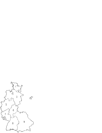
Figure 7: The subdivision of West Germany into eleven federal states (from Weidlich and Haag, 1988).

In the following, the results for migration in West Germany shall be presented. West Germany is divided into 10 federal states and the region of West Berlin (see figure 7 and table 1). The data for these $S=11$ regions can be found in the Statistische Jahrbücher of the years 1960 to 1985 on an annual basis ($t_{0}=1960$, $t_{1}=1961$, $\dots$, $t_{L}=1985$). Our data analysis will assume—with respect to migration—one more or less homogeneous population, that means, we have $A=1$, and the index $a$ can be dropped. Figure 8 shows some examples for the temporal variation of the effective transition rates $w_{\rm e}(x^{\prime}|x;t_{l})$.

Using the method of steepest descent, the minimization of the error function (49), (50) gives the following results:

$$\nu^{\rm 2}(t_{l})\approx 0\,,$$ (57)

that means, avoidance processes are negligible. The rate $\nu^{\rm e}(t_{l})$ of spontaneous behavioral changes and the rate $\nu^{1e}(t_{l})$ of imitative processes are depicted in figure 9. The utility functions $U^{\rm e}(x,t_{l})$ for spontaneous changes and the utility functions $U_{\rm e}(x,t_{l})$ for imitative processes are illustrated in figures 10 and 11.

The irregulatity of the utility functions $U_{\rm e}(x,t_{l})$ indicates that they probably fit random fluctuations of the migration data. Indeed, a mathematical analysis proves that the term

$$\nu^{1}(t_{l})P^{\rm e}(x,t_{l})\frac{\mbox{e}^{U(x^{\prime},t_{l})-U(x,t_{l})}}{D(x^{\prime},x;t_{l})}=\nu^{\rm 1e}(t_{l})P^{\rm e}(x,t_{l})\frac{\mbox{e}^{U_{\rm e}(x^{\prime},t_{l})-U_{\rm e}(x,t_{l})}}{D^{\rm e}(x^{\prime},x;t_{l})}$$ (58)

only explains 5.2 percent of the variance of the effective transition rates $w_{\rm e}(x^{\prime}|x;t)$. Therefore, it makes no significant contribution to their mathematical description, and the migration rates $w_{\rm e}(x^{\prime}|x;t)$ of West Germany can already be represented by the model

$$w(x^{\prime}|x;t_{l}):=\nu(t_{l})\frac{\mbox{e}^{U(x^{\prime},t_{l})-U(x,t_{l})}}{D(x^{\prime},x;t_{l})}=\nu^{\rm e}(t_{l})\frac{\mbox{e}^{U^{\rm e}(x^{\prime},t_{l})-U^{\rm e}(x,t_{l})}}{D^{\rm e}(x^{\prime},x;t_{l})}\,.$$ (59)

This result agrees with the model of Weidlich and Haag (1988)! Figure 12 shows the corresponding rate $\nu^{\rm e}(t_{l})$ of spontaneous changes, and figure 13 depicts the utility functions $U^{\rm e}(x,t_{l})$. The distances $D^{\rm e}(x^{\prime},x;t_{l})$ can be calculated from the formulas (50), (52), and (56). They are not only a measure for the mean geographical distances, but also for transaction costs (e.g., removal costs) and psychical differences (of the language, mentality, etc.).

The replacement of the time dependent distances $D^{\rm e}(x^{\prime},x;t_{l})$ with the time independent values $D_{*}^{\rm e}(x^{\prime},x)$ defined by

$$\frac{1}{D_{*}^{\rm e}(x^{\prime},x)}:=\frac{1}{L+1}\sum_{l=0}^{L}\frac{1}{D^{\rm e}(x^{\prime},x;t_{l})}$$ (60)

(see table 2) allows for a further model reduction. The optimal value of the rate of spontaneous behavioral changes is, then, given by

$$\nu_{*}^{\rm e}(t_{l}):=\nu^{\rm e}(t_{l})\cdot\sum_{x,x^{\prime}=1\atop(x^{\prime}\neq x)}^{{}\atop S}\frac{1}{D^{\rm e}(x^{\prime},x;t_{l})}\,.$$ (61)

Although the reduced model

$$w(x^{\prime}|x;t_{l}):=\nu_{*}^{\rm e}(t_{l})\frac{\mbox{e}^{U^{\rm e}(x^{\prime},t_{l})-U^{\rm e}(x,t_{l})}}{D_{*}^{\rm e}(x^{\prime},x)}$$ (62)

only needs $(S+1)\cdot(L+1)+S\cdot(S-1)/2=367$ variables for the description of $S\cdot(S-1)\cdot(L+1)=2860$ effective transition rates $w^{\rm e}(x^{\prime}|x;t_{l})$, it attains a very good correlation of 0.984 with the empirical data. For a more detailled discussion of this model, see Weidlich and Haag (1988).

6 Summary and outlook

In this article, a behavioral model has been proposed that incorporates in a consistent way many models of social theory: the diffusion models, the multinomial logit model, Lewin’s field theory, the logistic equation, the gravity model, the Weidlich-Haag model, and the game dynamical equations. This very general model opens new perspectives concerning a theoretical description and understanding of behavioral changes, since it is formulated fully mathematically. It takes into account spontaneous (or externally induced) behavioral changes and behavioral changes due to pair interactions. Two important kinds of pair interactions have been distinguished: imitative processes and avoidance processes. The model turns out to be suitable for computational simulations, but it can also be applied to concrete empirical data.

6.1 Memory effects

The formulation of the model in the previous sections has neglected memory effects that may also influence behavioral changes. However, memory effects can be easily included by generalizing the Boltzmann-like equations to

$$\frac{d}{dt}P_{a}(\mbox{\boldmath$x$},t)=\int\limits_{t_{0}}^{t}dt^{\prime}\sum_{x^{\prime}\in\Omega}\Big{[}w_{t-t^{\prime}}^{a}(\mbox{\boldmath$x$}|\mbox{\boldmath$x$}^{\prime};t^{\prime})P_{a}(\mbox{\boldmath$x$}^{\prime},t^{\prime})-w_{t-t^{\prime}}^{a}(\mbox{\boldmath$x$}^{\prime}|\mbox{\boldmath$x$};t^{\prime})P_{a}(\mbox{\boldmath$x$},t^{\prime})\Big{]}$$ (63a)

with the effective transition rates

$$w_{t-t^{\prime}}^{a}(\mbox{\boldmath$x$}^{\prime}|\mbox{\boldmath$x$};t^{\prime}):=w^{t-t^{\prime}}_{a}(\mbox{\boldmath$x$}^{\prime}|\mbox{\boldmath$x$};t^{\prime})+\sum_{b=1}^{A}\sum_{y\in\Omega}\sum_{y^{\prime}\in\Omega}w^{t-t^{\prime}}_{ab}(\mbox{\boldmath$x$}^{\prime},\mbox{\boldmath$y$}^{\prime}|\mbox{\boldmath$x$},\mbox{\boldmath$y$};t^{\prime})P_{b}(\mbox{\boldmath$y$},t^{\prime})\,,$$ (63b)

and generalizing the Boltzmann-Fokker-Planck equations to

$$\begin{array}[]{rcl}\displaystyle\frac{\partial}{\partial t}P_{a}(\mbox{\boldmath$x$},t)&=&\displaystyle\int\limits_{t_{0}}^{t}dt^{\prime}\,\bigg{\{}-\sum_{i=1}^{n}\frac{\partial}{\partial x_{i}}\Big{[}K_{ai}^{t-t^{\prime}}(\mbox{\boldmath$x$},t^{\prime})P_{a}(\mbox{\boldmath$x$},t^{\prime})\Big{]}\\ &&\qquad\quad\displaystyle+\frac{1}{2}\sum_{i,j=1}^{n}\frac{\partial}{\partial x_{i}}\frac{\partial}{\partial x_{j}}\Big{[}Q_{aij}^{t-t^{\prime}}(\mbox{\boldmath$x$},t^{\prime})P_{a}(\mbox{\boldmath$x$},t^{\prime})\Big{]}\bigg{\}}\end{array}$$ (64a)

with the effective drift coefficients

$$K_{ai}^{t-t^{\prime}}(\mbox{\boldmath$x$},t^{\prime}):=\int\limits_{\Omega}\!d^{n}x^{\prime}\,(x^{\prime}_{i}-x_{i})w^{a}_{t-t^{\prime}}(\mbox{\boldmath$x$}^{\prime}|\mbox{\boldmath$x$};t^{\prime})\,,$$ (64b)

the effective diffusion coefficients

$$Q_{aij}^{t-t^{\prime}}(\mbox{\boldmath$x$},t^{\prime}):=\int\limits_{\Omega}\!d^{n}x^{\prime}\,(x^{\prime}_{i}-x_{i})(x^{\prime}_{j}-x_{j})w^{a}_{t-t^{\prime}}(\mbox{\boldmath$x$}^{\prime}|\mbox{\boldmath$x$};t^{\prime})\,,$$ (64c)

and

$$w_{t-t^{\prime}}^{a}(\mbox{\boldmath$x$}^{\prime}|\mbox{\boldmath$x$};t^{\prime}):=w^{t-t^{\prime}}_{a}(\mbox{\boldmath$x$}^{\prime}|\mbox{\boldmath$x$};t^{\prime})+\sum_{b=1}^{A}\int\limits_{\Omega}d^{n}y\int\limits_{\Omega}d^{n}y^{\prime}\,w^{t-t^{\prime}}_{ab}(\mbox{\boldmath$x$}^{\prime},\mbox{\boldmath$y$}^{\prime}|\mbox{\boldmath$x$},\mbox{\boldmath$y$};t^{\prime})P_{b}(\mbox{\boldmath$y$},t^{\prime})\,.$$ (64d)

Obviously, in these formulas there only appears an additional integration over past times $t^{\prime}$ (Helbing, 1992c). The influence of the past results in a dependence of $w_{t-t^{\prime}}^{a}(\mbox{\boldmath$x$}^{\prime}|\mbox{\boldmath$x$};t^{\prime})$, $K_{ai}^{t-t^{\prime}}(\mbox{\boldmath$x$},t^{\prime})$, and $Q_{aij}^{t-t^{\prime}}(\mbox{\boldmath$x$},t^{\prime})$ on $(t-t^{\prime})$. The Boltzmann-like equations (2) resp. the Boltzmann-Fokker-Planck equations (21b) used in the previous sections result from (6.1) resp. (63b) in the limit of short memory.

6.2 Group dynamics

The force model described in section 3 can serve as a new mathematical modelling concept. For example, it has successfully been applied to the simulation of pedestrian behavior (cf. Helbing, 1991).

Another interesting field is an application of the force model to group dynamics and group formation. In this case we take $A=N$, that means, each subpopulation consists of one individual only ($N_{a}=1$). Since $N_{a}\gg 1$ is violated, then, the temporal change $dP_{a}(\mbox{\boldmath$x$},t)/dt$ of $P_{a}(\mbox{\boldmath$x$},t)$, which describes the probability of individual $a$ to show the behavior $x$ at time $t$, is additionally subject to fluctuations (cf. Helbing, 1992a,c). The interaction rates $\nu_{ab}\equiv\widetilde{\nu}_{ab}$ are related to the adjacency matrix and describe the social (interpersonal) network (Burt, 1982). Moreover, the sympathy matrix $\Big{(}s_{ab}(t)\Big{)}$ is affected by the social processes. The crucial task for simulating group dynamics is, therefore, to set up equations for the temporal change of $s_{ab}(t)$. The topic of group dynamics will be treated in a forthcoming paper.

Acknowledgements

This work has been financially supported by the Volkswagen Stiftung and the Deutsche Forschungsgemeinschaft (SFB 230). The author is grateful to Prof. Dr. W. Weidlich and Dr. R. Reiner for valuable discussions and commenting on the manuscript.

Figure 1: Imitative processes in the case of one-sided sympathy and low indifference $L_{a}$ with respect to behavioral changes.

Figure 2: As figure 1, but for high indifference $L_{a}$ with respect to behavioral changes.

Figure 3: Imitative processes for mutual sympathy and low indifference $L_{a}$ in both subpopulations.

Figure 4: As figure 3, but for high indifference $L_{2}$ in subpopulation 2.

Figure 5: Avoidance processes for mutual dislike of both subpopulations.

Figure 6: Avoidance processes for one-sided dislike.

symbol	region $x$	name
$+$	1	Schleswig-Holstein
$\odot$	2	Hamburg
$\bigtriangleup$	3	Niedersachsen
$\Box$	4	Bremen
$\Diamond$	5	Nordrhein-Westfalen
$\oplus$	6	Hessen
$\Join$	7	Rheinland-Pfalz
$\times$	8	Baden-Württemberg
$\bigtriangledown$	9	Bayern
$\setminus$	10	Saarland
/	11	Berlin

Table 1: The eleven federal states of West Germany, their names, and the symbols used in the following figures.

Figure 8: Time dependence of some effective transition rates of migration in West Germany.

Figure 9: Rate $\nu^{\rm e}(t_{l})$ of spontaneous behavioral changes ($\Box$) and rate $\nu^{\rm 1e}(t_{l})$ of imitative processes ($\bigtriangleup$) calculated from the migration data of West Germany.

Figure 10: Utility functions for spontaneous removals from one federal state to another in West Germany.

Figure 11: Utility functions for removals from one federal state to another due to imitative processes.

Figure 12: Rate of spontaneous migration in West Germany for the model of Weidlich and Haag.

Figure 13: Utility functions of the federal states of West Germany for the model of Weidlich and Haag. Note, that the utility of West Berlin (/) is extremely dependent on changes of the political situation. For example, there is an remarkable increase of the utility after the erection of the Berlin wall in the year 1961.

$x$	1	2	3	4	5	6	7	8	9	10	11
1	–	0.16	0.56	1.19	0.99	1.93	3.01	1.79	2.13	8.35	1.26
2	0.16	–	0.44	1.65	1.58	2.18	5.03	2.34	2.61	12.89	1.55
3	0.56	0.44	–	0.25	0.44	0.90	2.13	1.26	1.55	6.38	0.79
4	1.19	1.65	0.25	–	1.91	3.10	6.16	3.31	4.30	17.37	2.58
5	0.99	1.58	0.44	1.91	–	0.65	0.53	0.79	0.93	2.56	0.92
6	1.93	2.18	0.90	3.10	0.65	–	0.47	0.61	0.75	2.23	1.15
7	3.01	5.03	2.13	6.16	0.53	0.47	–	0.59	1.39	0.54	2.33
8	1.79	2.34	1.26	3.31	0.79	0.61	0.59	–	0.38	1.56	1.14
9	2.13	2.61	1.55	4.30	0.93	0.75	1.39	0.38	–	3.49	1.09
10	8.35	12.89	6.38	17.37	2.56	2.23	0.54	1.56	3.49	–	5.07
11	1.26	1.55	0.79	2.58	0.92	1.15	2.33	1.14	1.09	5.07	–

Table 2: Time independent effective distances $D^{\rm e}_{*}(x^{\prime},x)$ between the eleven federal states of West Germany.

References

• [1] [-2cm]
• [2] Axelrod, R. (1984) The Evolution of Cooperation. Basic Books, New York.
• [3] Bartholomew, D. J. (1967) Stochastic Models for Social Processes. Wiley, London.
• [4] Boltzmann, L. (1964) Lectures on Gas Theory. University of California, Berkeley.
• [5] Burt, R. S. (1982) Towards a Structural Theory of Action. Network Models of Social Structure, Perception, and Action. Academic Press, New York.
• [6] Coleman, J. S. (1964) Introduction to Mathematical Sociology. The Free Press of Glencoe, New York.
• [7] Davydov, A. S. (1976) Quantum Mechanics: §75. 2nd edition, Pergamon Press, Oxford.
• [8] Domencich, Th. A., and McFadden, D. (1975) Urban Travel Demand. A Behavioral Analysis: pp. 61–69. North-Holland, Amsterdam.
• [9] Eigen, M. (1971) The selforganization of matter and the evolution of biological macromolecules. Naturwissenschaften 58: 465.
• [10] Eigen, M., and Schuster, P. (1979) The Hypercycle. Springer, Berlin.
• [11] Feistel, R., and Ebeling, W. (1989) Evolution of Complex Systems. Kluwer Academic, Dordrecht.
• [12] Festinger, L. (1957) A Theory of Cognitive Dissonance. Row & Peterson, Evanston, IL.
• [13] Fisher, R. A. (1930) The Genetical Theory of Natural Selection. Oxford University Press, Oxford.
• [14] Fokker, A. D. (1914) Ann. Phys. 43: 810.
• [15] Forsythe, G. E., Malcolm, M. A., and Moler, C. B. (1977) Computer Methods for Mathematical Computations. Prentice Hall, Englewood Cliffs, N.J.
• [16] Granovetter, M. (1983) Threshold models of diffusion and collective behavior. Journal of Mathematical Sociology 9: 165–179.
• [17] Greenwood, D. T. (1988) Principles of Dynamics. 2nd edition, Prentice-Hall, Englewood Cliffs, N.J.
• [18] Heider, F. (1946) Attitudes and cognitive organization. Journal of Psychology 21: 107–112.
• [19] Helbing, D. (1991) A mathematical model for the behavior of pedestrians. Behavioral Science 36: 298–310.
• [20] Helbing, D. (1992a) Interrelations between stochastic equations for systems with pair interactions. Physica A 181: 29–52.
• [21] Helbing, D. (1992b) A mathematical model for attitude formation by pair interactions. Behavioral Science 37: 190–214.
• [22] Helbing, D. (1992c) Stochastische Methoden, nichtlineare Dynamik und quantitative Modelle sozialer Prozesse. PhD thesis, University of Stuttgart. Published by Shaker, Aachen, 1993.
• [23] Helbing, D. (1992d) A fluid-dynamic model for the movement of pedestrians. Complex Systems 6: 391–415.
• [24] Helbing, D. (1992e) A mathematical model for behavioral changes by pair interactions. In: G. Haag, U. Mueller, and K. G. Troitzsch (eds.) Economic Evolution and Demographic Change, pp. 330–348. Springer, Berlin.
• [25] Helbing, D. (1993) Stochastic and Boltzmann-like models for behavioral changes, and their relation to game theory. Physica A 193: 241–258.
• [26] Hofbauer, J., and Sigmund, K. (1988) The Theory of Evolution and Dynamical Systems. Cambridge University Press, Cambridge.
• [27] Kennedy, A. M. (1983) The adoption and diffusion of new industrial products: A literature review. European Journal of Marketing 17(3): 31–88.
• [28] Kramers, H. A. (1940) Physica 7: 284.
• [29] Kruskal, J. B., and Wish, M. (1978) Multidimensional Scaling. Sage, Beverly Hills.
• [30] Langevin, P. (1908) Comptes. Rendues 146: 530.
• [31] Lewin, K. (1951) Field Theory in Social Science. Harper & Brothers, New York.
• [32] Moyal, J. E. (1949) J. R. Stat. Soc. 11: 151–210.
• [33] von Neumann, J., and Morgenstern, O. (1944) Theory of Games and Economic Behavior. Princeton University Press, Princeton.
• [34] Newton, I. (1687) Philosophiae Naturalis Principia Mathematica.
• [35] Ortúzar, J. de D., and Willumsen, L. G. (1990) Modelling Transport. Wiley, Chichester.
• [36] Osgood, Ch. E., Suci, G. J., and Tannenbaum, P. H. (1957) The Measurement of Meaning: Chapter 6. University of Illinois Press, Urbana.
• [37] Osgood, Ch. E., and Tannenbaum, P. H. (1955) The principle of congruity in the prediction of attitude change. Psychological Review 62: 42–55.
• [38] Pearl, R. (1924) Studies in Human Biology. Williams & Wilkins, Baltimore.
• [39] Planck, M. (1917) Sitzungsber. Preuss. Akad. Wiss., p. 324.
• [40] Ravenstein, E. (1876) The birthplaces of the people and the laws of migration. The Geographical Magazine III: 173–177, 201–206, 229–233.
• [41] Schrödinger, E. (1926) Quantisierung als Eigenwertproblem. Annalen der Physik 79.
• [42] Schuster, P., Sigmund, K., Hofbauer, J., Wolff, R., Gottlieb, R., and Merz, Ph. (1981) Selfregulation of behavior in animal societies I–III. Biol. Cybern. 40: 1–25.
• [43] Statistische Jahrbücher 1960–1985, Wiesbaden
• [44] Stratonovich, R. L. (1963) Topics in the Theory of Random Noise, Vols. 1 & 2. Gordon and Breach, New York.
• [45] Verhulst, P. F. (1845) Nuov. Mem. Acad. Roy. Bruxelles 18: 1.
• [46] Weidlich, W. (1991) Physics and social science—The approach of synergetics. Physics Reports 204: 1–163.
• [47] Weidlich, W. (1994) Synergetic modelling concepts for sociodynamics with application to collective political opinion formation. Journal of Mathematical Sociology, in print.
• [48] Weidlich, W., and Haag, G. (1983) Concepts and Models of a Quantitative Sociology. The Dynamics of Interacting Populations. Springer, Berlin.
• [49] Weidlich, W., and Haag, G. (eds.) (1988) Interregional Migration. Springer, Berlin.
• [50] Young, F. W., and Hamer, R. M. (1987) Multidimensional Scaling: History, Theory, and Applications. Lawrence Erlbaum Associates, Hillsdale, N.J.
• [51] Zipf, G. K. (1946) The P1P2/D hypothesis on the intercity movement of persons. American Sociological Review 11: 677–686.
Refer to caption
Refer to caption
Refer to caption
Refer to caption
Refer to caption
Refer to caption