Adiabatic Charge Pumping in Almost Open Dots

Abstract

We consider adiabatic charge transport through an almost open quantum dot. We show that the charge transmitted in one cycle is quantized in the limit of vanishing temperature and one-electron mean level spacing in the dot. The explicit analytic expression for the pumped charge at finite temperature is obtained for spinless electrons. The pumped charge is produced by both non-dissipative and dissipative currents. The latter are responsible for the corrections to charge quantization which are expressed through the conductance of the system.

Adiabatic charge pumping occurs in a system subjected to a slow periodic perturbation. Upon the completion of the cycle, the Hamiltonian of the system returns to its initial form, however, a finite charge may be transmitted through some cross-section of the system. The natural question is what is the value of this charge transmitted through the system during one cycle, $Q$. This question does not have a universal answer. Thouless[1] showed that for certain one dimensional systems with a gap in the excitation spectrum in the thermodynamic limit the charge $Q$ is quantized. Such quantized charge pumping could be of practical importance as a standard of electric current[2]. The accuracy of charge quantization depends on the degree of adiabaticity of the process.

The practical attempts at creating a quantized electron pump use a different approach based on the phenomenon of Coulomb blockade[3, 4]. In this kind of devices, one uses several single electron transistors (SET) connected in series to increase the accuracy of charge quantization. At least two SET’s are necessary to obtain a non-zero charge transfer during one cycle.

Recently, another family of the Coulomb blockade devices was demonstrated[5] – semiconductor based quantum dots. The advantage of these devices is the possibility of changing not only the gate voltage and thus the average electron number in the dot but also the conductance of the quantum point contacts (QPC’s) separating the dot from the leads. By doing so, one can traverse from almost classical Coulomb blockade to the completely open dot where the effects of the charge quantization are diminished.

Having those semiconductor structures in mind, we theoretically study in this Letter the following setup for the adiabatic quantum pump. The device is depicted in Fig. 1 and consists of a quantum dot connected to two reservoirs labeled by $\alpha=\pm 1$ by one channel QPC’s characterized by reflection amplitudes $r_{\alpha}(t)$ and capacitively coupled to the metallic gate G. The gate potential is characterized by the number of electrons $N$ which minimizes the electrostatic energy of the dot. Experiments with a similar setup were reported in Ref. [6].

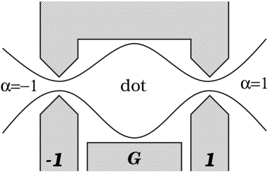
FIG. 1.: Schematic drawing of a quantum dot electrostatically defined on a surface of a two dimensional electron gas. The dot is connected to two leads by single channel QPC’s labeled by $\alpha$. The voltages on the gates “$G$” and “$\pm 1$” determine respectively the average electron number in the dot, $N(t)$, and the reflection amplitudes, $r_{\pm 1}(t)$, in the QPC’s.

We show below that the charge adiabatically transfered in one cycle is quantized in the limit of zero temperature and zero mean level spacing $\Delta$. For spinless electrons it is given by

$$\frac{Q}{e}=\frac{1}{2\pi i}\oint\frac{dz}{z},\quad z(t)=\sum_{\alpha}r_{\alpha}(t)e^{i\alpha\pi N(t)}.$$ (1)

We assume that during the cycle the system does not go through the degeneracy point $z=0$. The degree of adiabaticity of the process depends on the proximity to this degeneracy point.

To illustrate this quantization qualitatively, let us first consider the following trivial limit of the pumping cycle: i) the right contact ($\alpha=+1$) is completely pinched off, ii) the gate voltage is changed from $0$ to $N_{0}$, iii) the left contact ($\alpha=-1$) is adiabatically closed. In this process the average charge on the dot changes from $N_{0}$ to the nearest integer $n_{0}$ (If $N_{0}$ is not a degeneracy point, which is assumed, $n_{0}$ is unique), iv) the right contact is opened, and the gate voltage is changed from $N_{0}$ back to $0$, v) the left contact is opened. As a result of this cycle the total charge transfered from left to right is an integer $n_{0}$. The non-trivial statement is that even for contacts which stay weakly reflecting at all times during the cycle the total transfered charge is still quantized and is given by Eq. (1).

We assume that the electrons in the leads are non-interacting, and the interaction between the electrons on the dot is described by the standard model of Coulomb blockade for strong tunneling[7, 8], see Sec. 4.3 of Ref. [9] for the discussion of the applicability of this model. If the dot is connected to the leads of by single channel QPC’s the system can be treated within the one-dimensional effective Hamiltonian[7, 8] (we put $\hbar=k_{B}=1$ everywhere)

$$\hat{H}(t) = iv_{F}\sum_{\alpha}\int_{-\infty}^{+\infty}dx\left(\psi^{\dagger}_{L,\alpha}(x)\partial_{x}\psi_{L,\alpha}(x)-\psi^{\dagger}_{R,\alpha}(x)\partial_{x}\psi_{R,\alpha}(x)\right)+v_{F}\sum_{\alpha}\left(r_{\alpha}(t)\psi^{\dagger}_{R,\alpha}(0)\psi_{L,\alpha}(0)+h.c.\right)$$ (2)

$$+ E_{c}\left(\sum_{\alpha}\int^{+\infty}_{0}dx:\psi^{\dagger}_{L,\alpha}(\alpha x)\psi_{L,\alpha}(\alpha x)+\psi^{\dagger}_{R,\alpha}(\alpha x)\psi_{R,\alpha}(\alpha x):+N(t)\right)^{2}.$$ (3)

The first two terms in Eq. (3) describe the non-interacting electrons in the left ($\alpha=-1$) and the right ($\alpha=+1$) QPC respectively: the first term is the linearized version of the kinetic energy ($v_{F}$ is the Fermi velocity) and the second term corresponds to backscattering in the QPC’s. We restrict ourselves to the case of small reflection amplitudes, $r_{\alpha}(t)\ll 1$. Finally, the last term describes the effect of the Coulomb blockade in the dot, and $E_{C}$ is its charging energy. For simplicity, we explicitly consider the case of spinless electrons, the results for the electrons with spins will be presented at the end of the paper. The only difference of our Hamiltonian from those considered before[7, 8, 9] resides in its time dependence. Since upon the completion of the cycle the total charge of the dot returns to its original value the integrated current can be calculated through any cross-section of the system. For convenience we take half the sum of the currents flowing through the left and right point contacts:

$$\hat{I}=\frac{ev_{F}}{2}\sum_{\alpha}\left(:\psi^{\dagger}_{L,\alpha}(0)\psi_{L,\alpha}(0)-\psi^{\dagger}_{R,\alpha}(0)\psi_{R,\alpha}(0):\right),$$ (4)

where $e$ is the electron charge.

Similarly to Ref. [8], the Hamiltonian (3) can be bosonized according the rules

$$\psi_{L/R,\alpha}(x)=\frac{\hat{\eta}_{\alpha}}{\sqrt{2\pi\lambda}}\exp\left(\pm i\frac{\hat{\phi}^{I}_{L/R,\alpha}(x)+\alpha\hat{\phi}^{C}_{L/R,\alpha}(x)}{\sqrt{2}}\right)$$ (5)

where $\hat{\eta}_{\alpha}$ are Majorana fermions ($\hat{\eta}_{\alpha}=\hat{\eta}_{\alpha}^{\dagger}$, $\{\hat{\eta}_{\alpha},\hat{\eta}_{\alpha^{\prime}}\}=2\delta_{\alpha,\alpha^{\prime}}$), whereas the scale $\lambda$ characterizes the large momentum cut-off and is of the order of the Fermi wavelength.

Instead of the left and the right modes in Eq. (5) it is convenient to introduce the even and odd modes $\hat{\phi}^{I,C}_{\pm}$ as

$$\hat{\phi}^{i}_{L/R}(x)=\frac{\hat{\phi}^{i}_{+}(\pm x)\pm\hat{\phi}^{i}_{-}(\pm x)}{\sqrt{2}};\quad i=I,C.$$ (6)

The bosonic operators $\hat{\phi}^{I,C}_{\pm}(x)$ satisfy the following commutation relations

$$\left[\hat{\phi}^{i}_{+}(x),\hat{\phi}^{j}_{+}(y)\right]=\left[\hat{\phi}^{i}_{-}(x),\hat{\phi}^{j}_{-}(y)\right]=-i\pi{\rm sgn}(x-y)\delta_{ij}$$ (7)

$$\left[\hat{\phi}^{i}_{-}(x),\hat{\phi}^{j}_{+}(y)\right]=i\pi\delta_{ij};\quad i,j=I,C.$$ (8)

The last of Eqs. (8) ensures the correct anticommutation relation between left and right moving fermions, however, this subtlety will not be important for the problem in hand.

The odd modes $\hat{\phi}^{i}_{-}$ are decoupled from the rest of the Hamiltonian and do not contribute to the current (4), hence we can omit them. The relevant part of the Hamiltonian (3) acquires the following form

$$\hat{H}(t)=\frac{v_{F}}{4\pi}\!\sum_{i=I,C}\!\int_{-\infty}^{+\infty}\!\!\!\!dx\left(\frac{\partial\hat{\phi}^{i}_{+}(x)}{\partial x}\right)^{2}+E_{c}\left[\frac{\hat{\phi}^{C}_{+}(0)}{\pi}-N\right]^{2}$$ (9)

$$\ +\frac{v_{F}}{2\pi\lambda}\sum_{\alpha}\left\{r_{\alpha}(t)\exp\left[i\alpha\hat{\phi}^{C}_{+}(0)+i\hat{\phi}^{I}_{+}(0)\right]+h.c.\right\},$$ (10)

where the complex function of time $z(t)$ is given by Eq. (1). The bosonized current operator (4) becomes

$$\hat{I}=\left.\frac{ev_{F}}{2\pi}\frac{\partial\hat{\phi}^{I}_{+}}{\partial x}\right|_{x=0}.$$ (11)

As one can see from Eq. (10), the mode $\phi_{+}^{C}(0)$ is pinned by the charging energy $E_{C}$ to the value $\pi N$. Since $E_{C}$ is the large scale in the problem, for the description of the low energy dynamics of the system we can integrate $\phi_{+}^{C}$ out[7] and obtain the Hamiltonian of the form

$$\hat{H}^{\prime}(t) = \frac{v_{F}}{4\pi}\int_{-\infty}^{+\infty}dx\left(\frac{\partial\hat{\phi}^{I}_{+}(x)}{\partial x}\right)^{2}$$ (12)

$$+ \sqrt{\frac{\gamma v_{F}E_{C}}{2\pi^{3}\lambda}}\left[z(t)\exp(i\hat{\phi}^{I}_{+}(0))+h.c.\right],$$ (13)

where $\ln\gamma={\bf C}\approx 0.5772$ is the Euler constant.

The Hamiltonian (12) reduces to a non-interacting form through the introduction of the fermion fields[7]

$$\hat{\Psi}(x)=\frac{\hat{\zeta}}{\sqrt{2\pi\lambda}}\exp\left(i\hat{\phi}^{I}_{+}(x)\right),$$ (14)

where $\hat{\zeta}$ is a Majorana fermion.

The re-fermionized Hamiltonian (12) can be conveniently written in a matrix form

$$\hat{H}_{F}(t) = \frac{1}{2}\int_{-\infty}^{+\infty}dx\hat{\Upsilon}^{\dagger}(x)\hat{H}_{0}\hat{\Upsilon}(x),$$ (16)

$$\hat{\Upsilon}^{\dagger}(x) = \left(\hat{\Psi}^{\dagger}(x),\hat{\Psi}(x),\zeta\right),$$ (17)

$$\hat{H}_{0} = \pmatrix{-iv_{F}\partial_{x}&0&\kappa z^{*}(t)\delta(x)\cr 0&iv_{F}\partial_{x}&-\kappa z(t)\delta(x)\cr\kappa z(t)\delta(x)&\kappa z^{*}(t)\delta(x)&0\cr},$$ (18)

where $\kappa=\sqrt{\gamma v_{F}E_{c}/\pi^{2}}$. The re-fermionized current operator (11) acquires the form

$$\hat{I}_{F}=ev_{F}:\hat{\Psi}^{\dagger}(0)\hat{\Psi}(0):$$ (19)

Next, we define the matrix Green function $\hat{G}^{<}(t,t^{\prime};x,x^{\prime})$ which includes both normal and anomalous components

$$\hat{G}(t,t^{\prime};x,x^{\prime}) = -i\left\langle T_{t}\hat{\Upsilon}(x,t)\otimes\hat{\Upsilon}^{\dagger}(x^{\prime},t^{\prime})\right\rangle$$ (20)

where $\langle\ldots\rangle$ denotes averaging over the quantum state of the system. The retarded and advanced Green functions $\hat{G}^{R/A}(t,t^{\prime};y,y^{\prime})$ are defined in a similar manner.

All of the observables can be expressed through the Green function at almost coinciding times, $\hat{{\cal G}}(t;x,x^{\prime})$

$$\hat{{\cal G}}(t;x,x^{\prime})=\hat{G}(t,t+0;x,x^{\prime}),$$ (21)

where $\hat{G}(t,t^{\prime};x,x^{\prime})$ is defined in Eq. (20). For example, the instantaneous current through the system is given by

$$I(t)=-iev_{F}\hat{{\cal G}}_{11}(t;x=0,x^{\prime}=0).$$ (22)

In the leading adiabatic approximation the Green functions of the system coincide with those in equilibrium at the instantaneous value of $z$, and the current (22) vanishes. Therefore, to find the current flowing through the system in response to an adiabatic change of the Hamiltonian we have to find the first non-adiabatic correction to the Green function (21). It obeys the evolution equation

$$\frac{d\hat{\cal G}(t)}{dt}=-i\left[\hat{H}_{0}(t),\hat{\cal G}(t)\right],$$ (23)

where $\hat{H}_{0}(t)$ is given by Eq. (18). From this equation it follows that the first non-adiabatic correction to the Green function (21) is given by

$$\delta\hat{\cal G}(t)=-\int\frac{d\omega}{2\pi}\hat{G}^{R}_{0}\left[z(t),\omega\right]\frac{d\hat{\cal G}_{0}\left[z(t)\right]}{dt}\hat{G}^{A}_{0}\left[z(t),\omega\right],$$ (24)

where $\hat{\cal G}_{0}[z(t)]$ is the equilibrium Green function (21) for the instantaneous value of the parameter $z(t)$, and $\hat{G}_{0}^{R/A}[z(t),\omega]$ are the frequency representations for the retarded and advanced Green functions at fixed $z(t)$. They can be found from the following equations

$$\left(\omega_{\pm}{\rm diag}\left[1,1,1/2\right]-\hat{H}_{0}(x)\right)\hat{G}_{0}^{R/A}(z(t),\omega;x,x^{\prime})=$$ (26)

$$\hskip 42.67912pt{\rm diag}\left[\delta(x-x^{\prime}),\delta(x-x^{\prime}),1\right],$$ (27)

$$\hat{\cal G}_{0}\left[z(t)\right]=\int\frac{d\omega}{2\pi}n_{F}(\omega)\left(\hat{G}_{0}^{A}(z,\omega)-\hat{G}_{0}^{R}(z,\omega)\right),$$ (28)

where $n_{F}(\omega)=\left[1+\exp(\omega/T)\right]^{-1}$ is the Fermi distribution function, and $\omega_{\pm}\equiv\omega\pm i0$.

We solve Eq. (27) for the Green functions, substitute the result in Eqs. (28) and (24), and thus find the current (22). Integrating the result over the cycle period we find the charge transmitted during the cycle. It can be represented through the the dimensionless conductance of the system $g$ (in units of $e^{2}/2\pi\hbar$) as

$$Q=\frac{1}{2\pi i}\oint\frac{dz}{z}\left[1-2g(|z|^{2},T)\right],$$ (29)

where the dimensionless conductance is given by [8]

$\displaystyle g=\frac{1}{2}-\frac{\gamma|z(t)|^{2}E_{c}}{2\pi^{3}T}\zeta\left(2,\frac{1}{2}+\frac{|z(t)|^{2}\gamma E_{c}}{\pi^{3}T}\right),$with $\zeta\left(x,y\right)$ being the Riemann zeta-function. At low temperatures, $T\ll|z|^{2}E_{c}$, conductance vanishes as $g\propto T^{2}/(|z|^{2}E_{c})^{2}$, which means that the transmitted charge tends to its quantized value. At high temperatures $T\gtrsim|z|^{2}E_{c}$ the conductance approaches the classical value $g=1/2$, and the pumped charge (29) vanishes. In general, for $g\neq 0$, the pumped charge depends on the shape of the contour $z(t)$ and is not a topological number.

We stress that Eq. (29) for the transmitted charge is given by the sum of two terms: i) the first one arises from non-dissipative currents (This contribution is quantized and represents a topological invariant of the cycle.), and ii) the second one, containing the conductance, is due to dissipative currents generated by the cycling of the dot.

This fact is not accidental and becomes more transparent from the following consideration which applies to a more general class of systems. The time dependent Hamiltonian can be written as $\hat{H}(t)=\hat{A}^{\dagger}(t)\hat{H}_{0}(t)\hat{A}(t)$, where $\hat{H}_{0}$ is diagonal. In the adiabatic limit the transmitted charge can be most conveniently evaluated by going to the adiabatically rotating basis $|\tilde{\psi}_{i}(t)\rangle=\hat{A}(t)|\psi_{i}(t)\rangle$ (the “rotating axis representation”[10]), and calculating the current in response to the arising perturbation $i\partial_{t}\hat{A}(t)\hat{A}^{\dagger}(t)$ using the Kubo formula

$$I=-\int_{-\infty}^{0}dt\langle[\partial_{t}\hat{A}(t)\hat{A}^{\dagger}(t),\hat{I}(0)]\rangle.$$ (30)

Now let us apply Eq. (30) to the case of an open dot which is connected to the leads by two groups of channels denoted by index $\alpha_{i}=\pm 1$, and which is described by the Hamiltonian similar to Eq. (3). For this purpose we introduce the partial particle number operator in each channel

$$\hat{n}_{i}=\int_{0}^{\infty}dx\psi^{\dagger}_{i}(\alpha_{i}x)\psi_{i}(\alpha_{i}x)$$ (31)

We notice, that even though the average particle number $\langle\hat{n}_{i}\rangle_{H}$ in each channel is infinite, its change during the pumping cycle is a well defined quantity and is determined by the the gate voltage, $N(t)$ and the reflection coefficients $r_{j}$. The calculation is facilitated by the explicit form of the unitary operator

$$\hat{A}(t)=\prod_{j}\exp\left(\frac{i\pi\alpha_{j}\langle\hat{n}_{j}\rangle_{H}}{v_{F}}\int_{-\infty}^{+\infty}\!dx\ \hat{I}_{i}(x)\right),$$ (32)

where $\hat{I}_{j}(x)$ is the partial particle current operator in channel $j$ at point $x$,

$$\hat{I}_{j}(x)=\frac{i}{2m}\left[\psi_{j}^{\dagger}\partial_{x}\psi_{j}-\left(\partial_{x}\psi_{j}^{\dagger}\right)\psi_{j}\right].$$ (33)

Recalling that the time evolution of operators at $x\neq 0$ corresponds to free propagation with velocity $v_{F}$ we readily express the pumping current through the dimensionless partial conductances $g_{ij}$ between the channels

$$I=-\frac{e}{2}\sum_{i,j}\alpha_{j}\frac{d\langle\hat{n}_{i}\rangle_{H}}{dt}(\delta_{ij}-g_{ij}),$$ (34)

$$g_{ij}=2\pi i\int_{-\infty}^{0}dt\ t\left[\hat{I}_{i}(t,0);\hat{I}_{j}(0,0)\right].$$ (35)

For the model of spinless electrons, Eq. (34) reproduces Eq. (29), since $g_{1,-1}$ is the two terminal conductance of the system, $g_{1,1}=g_{1,-1}=g$ because of charge conservation, and $\langle\hat{n}_{1}+\hat{n}_{-1}\rangle_{H}=-N(t)$, because of the large charging energy. The explicit relation $\langle\hat{n}_{1}-\hat{n}_{-1}\rangle_{H}=-\frac{1}{\pi}{\rm Im}\ln z(t)$ with $z$ given by Eq. (1) requires the model assumption (3).

Equation (34) holds even in the case when the elastic cotunneling [11] can not be neglected. As shown in Ref. [9] the elastic returns in the strong tunneling case can be described by an $N$-independent action. Therefore, the explicit form of the unitary operator (32) and Eq. (34) are still valid. This observation gives us an estimate of $\Delta/(|z|^{2}E_{C})$ for the sample-specific[12, 9] correction to the quantized value of the charge due to the finite level spacing in the dot, $\Delta$, since the conductance in the valley of the CB remains finite even in the zero-temperature limit $g\simeq\Delta/(|z|^{2}E_{C})$[9].

Let us now apply Eq. (34) to strong inelastic cotunneling of electrons with spin. Because of the spin symmetry and charge conservation we have $\sum_{s}g_{\alpha,\alpha^{\prime}}^{s,s^{\prime}}=g/2$, where $s$ is the spin index and $g$ is the two terminal conductance, and we readily obtain

$$I=\ -\frac{e}{2}\sum_{\alpha,s}\alpha\frac{d\langle\hat{n}_{\alpha}^{s}\rangle_{H}}{dt}\left[1-g(t)\right].$$ (36)

At high temperature $g\to 1$, and pumping is suppressed, whereas at low temperatures the conductance vanishes as $T^{2}$ [8]. The explicit relation between $\langle\hat{n}_{\alpha}^{s}\rangle_{H}$ and the parameters of the Hamiltonian is a difficult problem which was not solved. However, for the anisotropic case, where the reflection coefficient in one contact is much stronger than in the other, one can show that $\sum_{\alpha,s}\alpha d\langle\hat{n}_{\alpha}^{s}\rangle_{H}/dt\approx\left(dN(t)/dt\right){\rm sgn}(\sum_{\alpha}\alpha|r_{\alpha}|)$. Moreover, if in the transition region, $r_{1}\sim r_{-1}$, we do not go through a degeneracy point $\cos\pi N=0$ the pumped charge remains quantized at zero temperature, and the problem is topologically equivalent to the spinless case. All estimates of the finite level spacing effect remain the same as for the spinless case.

To summarize, we considered adiabatic charge transport through a quantum dot. We have shown, that even in the case of small backscattering in the channel, when quantum fluctuations of the dot charge are large, the transmitted charge is still quantized. We have calculated corrections to the quantized value of the charge due to finite temperature and the level spacing in the dot. These corrections are expressed through the conductance $g$ and originate from the dissipative currents generated by pumping.

We are grateful to B.L. Altshuler, A. Ludwig, C.M. Marcus, B.Z. Spivak, and F. Zhou for interesting discussions. I.A. is an A.P. Sloan research fellow. A.A. is supported by NSF Grant No. PHY94-07194.

REFERENCES

- [1] D.J. Thouless, Phys. Rev. B 27, 6083 (1983).
- [2] Q. Niu, Phys. Rev. Lett. 64, 1812 (1990).
- [3] D.V. Averin and K. K. Likharev, in Mesoscopic Phenomena in Solids, Eds. B.L. Altshuler, P.A. Lee and R.A. Webb (Elsevier, Amsterdam, 1991).
- [4] M.H. Devoret, D. Esteve and C. Urbina, in Les Houches. Session LXI Mesoscopic Quantum Physics Eds. E. Akkermans, G. Montambaux, J.-L. Pichard and J. Zin-Justin (Elsevier, Amsterdam, 1995).
- [5] L.P. Kouwenhoven et. al. Proceedings of the Advanced Study Institute on Mesoscopic Electron Transport, Eds. L. Sohn, L.P. Kouwenhoven and G. Schoen (Kluwer, Series E, 1997).
- [6] L.P. Kouwenhoven et. al. Phys. Rev. Lett. 67, 1626 (1991)
- [7] K.A. Matveev, Phys. Rev. B51, 1743 (1995).
- [8] A. Furusaki and K.A. Matveev, Phys. Rev. Lett. 75, 709 (1995); Phys. Rev. B52, 166676 (1995).
- [9] I.L. Aleiner and L.I. Glazman, Phys. Rev. B, 57, 9608 (1998).
- [10] A. Messiah, Quantum Mechanics, vol.2, ch XVII, §11, (North-Holland Pub. Co.; New York : J. Wiley, 1962).
- [11] D.V. Averin and Yu.N. Nazarov, Phys. Rev. Lett. 65, 2446 (1990) .
- [12] I.L. Aleiner and L.I. Glazman, Phys. Rev. Lett. 77, 2057 (1996).