[

Persistent current and correlation effects in carbon nanotubes

Abstract

The persistent current of interacting electrons in toroidal single-wall carbon nanotubes is evaluated within Haldane’s concept of topological excitations. The overall pattern of the persistent current corresponds to the constant interaction model, whereas the fine structure stems from the electronic exchange correlations.

]

The recent breakthrough in the synthesis of a new generation of quantum wires - single-wall carbon nanotubes (SWNTs) [1] and the subsequent observation [2, 3] of coherent electron transport in this system have initiated a surge of experimental and theoretical activity (see e.g. Refs. [4, 5, 6, 7, 8, 9]) . The investigation of non-Fermi liquid correlation effects due to one-dimensional nature of interacting electrons in SWNTs presents one of the main challenges. The signatures of such correlations are often masked by the charging effects. Nevertheless, very recent experimental results [4] on the spin structure of the ground state suggest the interpretation in terms of electron correlations.

Generically, carbon nanotubes have linear or curved shape. Recently Liu et. al. [10] have observed individual circular SWNTs and ropes of such nanotubes. The experimental data suggests uniform widths of SWNTs and does not display the presence of their ends. For this reason it is plausible that circular SWNTs have the topology of a torus. One can test this conjecture by measuring the response of circular SWNTs to a weak perpendicular magnetic field. Since SWNTs are typically almost free from defects [1], the presence of delocalized electronic states in the system should result in a persistent current. To provide theoretical support for future experiments, we analyze the persistent current in toroidal SWNTs (TNTs).

We are aware of two recent papers [11, 12] where the persistent current in TNTs has been computed from first principles within the single-particle scheme. The results are either related to the specific fullerenes ($C_{576}$ carbon toroids [11]), or limited to the special case of half-filling [12]. Moreover, both works ignore electron correlations due to the Coulomb interaction, whose observable signatures in the pattern of the persistent current are investigated in this Letter.

We employ bosonization formalism [13] which has proven to be effective for analysis of persistent currents in various one-dimensional models [14]. First, we extend the bosonization scheme [7, 9, 15] (see also [8]) to the case of TNTs of the ”armchair” $(N,N)$ type. The Fermi operators $\Psi_{s}$ for electrons with spin $s=\pm$ can be expanded near the two crossing (or Fermi) points $\alpha K$ ($\alpha=\pm$, $K=4\pi/3a$) of the energy spectrum into right- ($d=+$) and left-moving ($d=-$) components, $\Psi_{s}(x)=\sum_{\alpha d}e^{i\alpha Kx}\psi_{asd}(x).$ The periodicity of the electronic fields $\Psi_{s}(x+L)=\Psi_{s}(x)$ results in the following boundary condition for the slowly-varying parts, $\psi_{asd}(x+L)=\psi_{asd}(x)e^{2\pi i\alpha p/3}$ where $p=0,\pm 1$ parametrizes the number $L/a$ of elementary cells along the nanotube of length $L$, $L/a=3n+p$ ($n$ is an integer).

Bosonization allows one to express the Fermi operators $\psi_{asd}(x)\propto e^{i(\phi_{\alpha s}+d\theta_{\alpha s})}$ in terms of the bosonic fields $\theta_{\alpha s}$ and $\phi_{\alpha s}$ obeying the commutation rules $\left[\theta_{\alpha s}(x),\phi_{\alpha^{\prime}s^{\prime}}(x^{\prime})\right]=(\pi i/2)\mbox{sign}(x-x^{\prime})\delta_{\alpha\alpha^{\prime}}\delta_{ss^{\prime}}$. The fields can be decomposed into topological parts and non-zero bosonic modes $\tilde{\theta}_{\alpha s}$, $\tilde{\phi}_{\alpha s}$:

$$\theta_{\alpha s}(x) = \theta_{\alpha s}^{(0)}+(N_{\alpha s}+1)\pi x/L+\tilde{\theta}_{\alpha s}(x),$$ (1)

$$\phi_{\alpha s}(x) = \phi_{\alpha s}^{(0)}+(J_{\alpha s}+2p\alpha/3)\pi x/L+\tilde{\phi}_{\alpha s}(x).$$ (2)

The pairs of the action-angle operators $J_{\alpha s},\theta_{\alpha s}^{(0)}$ and $N_{\alpha s},\phi_{\alpha s}^{(0)}$ satisfy the canonical commutation relation, $\left[N_{\alpha s},\phi_{\alpha^{\prime}s^{\prime}}^{(0)}\right]=\left[J_{\alpha s},\theta_{\alpha^{\prime}s^{\prime}}^{(0)}\right]=-i\delta_{\alpha\alpha^{\prime}}\delta_{ss^{\prime}}.$ The topological excitations $N_{\alpha s}$, $J_{\alpha s}$ are simply related to the numbers $M_{\alpha sd}=(N_{\alpha s}+dJ_{\alpha s})/2$ of excess electrons at the branch $\alpha$, $s$, $d$ of the energy spectrum, see inset of Fig. 1a. Since $M_{\alpha sd}$ are integers, the sum $N_{\alpha s}+J_{\alpha s}$ must be even (formally this topological constraint follows from the boundary condition on $\psi$-operators).

Following Refs. [7, 8, 9] we introduce bosonic fields $\theta_{\delta\nu}(x)$ and $\phi_{\delta\nu}(x)$ describing the charge $\nu=+$ and spin $\nu=-$ excitations in the symmetric $\delta=+$ and antisymmetric $\delta=-$ modes,

$$O_{\delta\nu}=[O_{++}+\nu O_{+-}+\delta(O_{-+}+\nu O_{--})]/2,$$ (3)

where $O=\theta$ ($\tilde{\theta},\theta^{(0)},N$) or $\phi$ ($\tilde{\phi},\phi^{(0)},J$) and the indices in the r.h.s. correspond to $\alpha$, $s$. The new fields,

$$\theta_{\delta\nu}(x) = \theta_{\delta\nu}^{(0)}+(N_{\delta\nu}+2\delta_{\delta+}\delta_{\nu+})\pi x/L+\tilde{\theta}_{\delta\nu}(x),$$ (4)

$$\phi_{\delta\nu}(x) = \phi_{\delta\nu}^{(0)}+(J_{\delta\nu}+(4/3)p\delta_{\delta-}\delta_{\nu+})\pi x/L+\tilde{\phi}_{\delta\nu}(x),$$ (5)

satisfy the commutation relations, $\left[\theta_{\delta\nu}(x),\phi_{\delta^{\prime}\nu^{\prime}}(x^{\prime})\right]=(\pi i/2)\mbox{sign}(x-x^{\prime})\delta_{\delta\delta^{\prime}}\delta_{\nu\nu^{\prime}}$, $\left[N_{\delta\nu},\phi_{\delta^{\prime}\nu^{\prime}}^{(0)}\right]=\left[J_{\delta\nu},\theta_{\delta^{\prime}\nu^{\prime}}^{(0)}\right]=-i\delta_{\delta\delta^{\prime}}\delta_{\nu\nu^{\prime}}$. The topological constraint for $N_{\alpha s}+J_{\alpha s}$ implies that $\sum_{\delta\nu}N_{\delta\nu}$, $\sum_{\delta\nu}J_{\delta\nu}$, $\sum_{\nu}N_{\delta\nu}+J_{\delta\nu}$, $\sum_{\delta}N_{\delta\nu}+J_{\delta\nu}$, all must be even, whereas $\sum_{\delta\nu}N_{\delta\nu}+J_{\delta\nu}=0\mbox{ mod }4$. In addition, the new topological numbers should be either all integer or all half-integer. Note that $N_{tot}=2N_{++}+4$, $2N_{++}=\sum_{\alpha sd}M_{\alpha sd}$ is the total number of extra electrons in the system [16], whereas $2J_{++}=\sum_{\alpha sd}dM_{\alpha sd}$ is the difference in numbers of right- and left-movers.

We concentrate first on the Luttinger model-like term [7, 9, 8] $H_{L}$ of the low-energy Hamiltonian $H=H_{L}+V$ of TNTs,

$$H_{L}=\sum_{\delta\nu} \int_{-L/2}^{L/2}\frac{dx}{2\pi}\left\{\frac{v_{\delta\nu}}{K_{\delta\nu}}\left(\nabla\theta_{\delta\nu}-\frac{2K_{\delta\nu}}{v_{\delta\nu}}\mu\delta_{\delta+}\delta_{\nu+}\right)^{2}\right.$$ (7)

$$\left.+v_{\delta\nu}K_{\delta\nu}\left(\nabla\phi_{\delta\nu}-\frac{2e}{c}A\delta_{\delta+}\delta_{\nu+}\right)^{2}\right\},$$

where the standard interaction parameters $K_{\delta\nu}$ and velocities $v_{\delta\nu}$ of excitations are introduced, so that $K_{\delta\nu}=1$ for non-interacting electrons. The electro-chemical potential $\mu$ of an electronic reservoir controls the charge density $\rho=2e\nabla\theta_{++}/\pi$. The vector potential $A$ of an external magnetic field is coupled to the persistent current $I=-2e\dot{\theta}_{++}/\pi$. We will neglect the Zeeman term $\mu_{B}H$ which is a factor $\sim a/L$ smaller than the energy scale $v_{F}/L$ of interest.

The Hamiltonian $H_{L}$ splits into the bosonic part $H_{b}$ (which has the form (7) with $\theta\to\tilde{\theta}$, $\phi\to\tilde{\phi}$, and $\mu=A=0$) and the topological part,

$$H_{t} = \frac{\pi}{2L}\sum_{\delta\nu}\frac{v_{\delta\nu}}{K_{\delta\nu}}\left[N_{\delta\nu}-4\left(f_{\mu}-\frac{1}{2}\right)\delta_{\delta+}\delta_{\nu+}\right]^{2}$$ (8)

$$+ v_{\delta\nu}K_{\delta\nu}\left[J_{\delta\nu}-4f_{\Phi}\delta_{\delta+}\delta_{\nu+}+\frac{4p}{3}\delta_{\delta-}\delta_{\nu+}\right]^{2}.$$ (9)

Here $f_{\Phi}=\Phi/\Phi_{0}$ is the magnetic flux $\Phi$ through the TNT in units of the flux quanta $\Phi_{0}=2\pi\hbar c/e$, and $f_{\mu}=(K_{++}L/2\pi v_{++})\mu$ is a normalized electro-chemical potential, whose reference point corresponds to the crossing of the energy spectrum. The increase of $f_{\mu}$ by one corresponds to the addition of an electron to each branch $\alpha$, $s$, $d$ of the spectrum, so that the properties of the system are periodic in $f_{\mu}$ with a period of one (the same periodicity occurs in $f_{\Phi}$). The Hamiltonian (9) shows additional symmetries with respect to changes in sign of the electro-chemical potential ($f_{\mu}\to-f_{\mu}$, $M_{\alpha sd}\to-M_{\alpha s-d}-1$) or the magnetic flux ($f_{\Phi}\to-f_{\Phi}$, $M_{\alpha sd}\to M_{-\alpha s-d}$).

The persistent current $I=dF/d\Phi$ can be calculated by differentiating the free energy ${F}$ of the system with respect to the magnetic flux $\Phi$,

$$I=(ev_{++}K_{++}/L)(8f_{\Phi}-2\langle J_{++}\rangle).$$ (10)

Due to the symmetries of the Hamiltonian, the persistent current is an even (odd) periodic function of $f_{\mu}$ ($f_{\Phi}$). At zero temperature the average $\langle J_{++}\rangle$ is determined by the ground state, whose map is given in Figs. 1,2. The persistent current (10) shows saw-tooth dependence on the magnetic flux and changes in a stepwise manner as a function of the electro-chemical potential. The amplitude of the persistent current is given by $I_{\max}=4ev_{++}K_{++}/L\approx 0.5$ $\mu$A, for $v_{++}K_{++}\simeq v_{F}\approx 8\times 10^{5}$ m/s and $L=1$ $\mu$m. This value is by two orders of magnitude larger than the persistent current measured in GaAs mesoscopic rings [17].

The unscreened long-range Coulomb interaction strongly influences the forward scattering of electrons leading to a large stiffness of the symmetric charge mode [7, 8], $K_{++}\approx 0.2$. We will first ignore the sublattice-dependent part of the forward scattering as well as the backscattering of electrons so that [8] $v_{++}=v_{F}/K_{++}$ and $K_{\delta\nu}=1$, $v_{\delta\nu}=v_{F}$ for the modes $(\delta\nu)=(+-),(-+),(--)$. Within this approximation, the energy spectrum of the topological Hamiltonian (9) is given by the sum of the Coulomb and single-particle energies, which corresponds to the constant interaction model (see e.g. Ref. [5]).

The ground state configurations for TNTs with $p=0,1$ are shown in Fig. 1. Due to the spin degeneracy, the eigenstates of the Hamiltonian (9) are characterized by four topological numbers, $M_{\alpha d}=\sum_{s}M_{\alpha sd}$, Fig. 1b. For the nanotubes with $p=0$ the states of electrons moving in the same direction at $\alpha=\pm$ are degenerate. The system can be described by the two numbers $M_{d}=\sum_{\alpha}M_{\alpha d}$ of extra right- and left-movers, Fig. 1a.

Since the Coulomb interaction in SWNTs is strong ($K_{++}\ll 1$), the electron number $N_{tot}$ is determined primarily by the electro-chemical potential, although in narrow regions it can be controlled by magnetic flux (Fig. 1). The slope of the ground state borders enables one to deduce the value of the interaction constant $K_{++}$ from experimental data [18]. Generically, the changes of the ground state with the magnetic flux correspond to the jumps of electrons between different branches of the spectrum and occur at universal values of magnetic flux - $f_{\Phi}=0,1/2$ for $p=0$ and $f_{\Phi}=0,1/6,1/3,1/2$ for $p=\pm 1$. In particular, the jump of an electron at zero flux causes the paramagnetic response of TNT. Such paramagnetic ground states occur if $N_{tot}\neq 4$ $\mathop{\rm mod}$ $8,$ for $p=0$, and $N_{tot}\neq 0$ $\mathop{\rm mod}$ $4$, for $p=\pm 1$ (see Fig. 1). Otherwise, the ground state is diamagnetic.

The sublattice-dependent part of the forward scattering and backscattering of electrons lead to the appearance of an essentially non-Luttinger term $V=V_{f}+V_{b}$ in the Hamiltonian and the renormalization of the parameters $K_{\delta\nu}$, $v_{\delta\nu}$ in Eq. (7). The Luttinger and non-Luttinger parts of the Hamiltonian describe intra- and interbranch scattering of electrons respectively. The derivation of these terms from a microscopic model has been discussed in Refs. [9, 7, 15] and here we present only the results for a generic case away from half-filling. The non-Luttinger terms are given by

$$V_{f} = \frac{\Delta V(0)}{2\pi^{2}\tilde{a}^{2}}\int_{-L/2}^{L/2}dx\{\cos 2\theta_{+-}\cos 2\theta_{--}$$ (12)

$$-\cos 2\theta_{-+}\cos 2\theta_{--}-\cos 2\theta_{-+}\cos 2\theta_{+-}\},$$

$$V_{b} = \frac{1}{\pi^{2}\tilde{a}^{2}}\int_{-L/2}^{L/2}dx\{\bar{V}(2K)\cos 2\theta_{+-}\cos 2\phi_{--}$$ (15)

$$+\frac{\Delta V(2K)}{2}[\cos 2\theta_{-+}\cos 2\theta_{--}+\cos 2\theta_{-+}\cos 2\phi_{--}$$

$$\hskip 49.79231pt+\cos 2\theta_{--}\cos 2\phi_{--}]\},$$

where the matrix elements $\bar{V}(q)=[V_{+}(q)+V_{-}(q)]/2$, $\Delta V(q)=V_{+}(q)-V_{-}(q)$ are related to the electron scattering amplitudes $V_{p}(q)$ given below, and $\tilde{a}\sim 1/K$ is the standard ultraviolet cutoff in the Luttinger model. The interaction constants $K_{\delta\nu}=\sqrt{B_{\delta\nu}/A_{\delta\nu}}$, and velocities of excitations $v_{\delta\nu}=v_{F}\sqrt{A_{\delta\nu}B_{\delta\nu}}$ (7) are defined by [9]

FIG. 1.: The ground state of TNTs with $p=0$ (a) and $p=1$ (b) in terms of the topological numbers $M_{d}=(M_{+},M_{-})$ (a) and $M_{\alpha d}=[M_{++},M_{+-},M_{-+},M_{--}]$ (b). The ground state changes at the solid lines. We choose $K_{++}=0.2$. Inset: Electronic states near the crossing point $\alpha=1$ of the spectrum for TNTs with $p=0$ (circles) $-1$ (squares) $1$ (triangles) at $f_{\Phi}=0$. The filling of the electronic states with the energy $E\leq 2\pi v_{F}/3L$ at the branch $\alpha,s,d$ corresponds to $M_{\alpha sd}=0$. The plot for $\alpha=-1$ can be obtained by symmetry with respect to $k=0$.

$$A_{++} = 1+\frac{4\bar{V}(0)}{\pi v_{F}}-\frac{\Delta V(0)}{4\pi v_{F}}-\frac{V_{+}(2K)}{2\pi v_{F}},$$ (16)

$$A_{\delta\nu} = 1-\frac{\Delta V(0)}{4\pi v_{F}}-\delta\frac{V_{+}(2K)}{2\pi v_{F}},$$ (17)

$$B_{\delta\nu} = 1+\frac{\Delta V(0)}{4\pi v_{F}}+\delta\frac{V_{-}(2K)}{2\pi v_{F}}.$$ (18)

Here $V_{+}(q)$ and $V_{-}(q)$ are the amplitudes of intrasublattice and intersublattice electron scattering with momentum transfer $q=0,2K$. The forward scattering ($q=0$) has the strongest amplitude, $\bar{V}(0)=2e^{2}\ln(R_{s}/R)/\kappa$, where $\kappa$ is an effective dielectric constant of the media (an estimate [7] for the parameters of the experiment [2] gives $\kappa=1.4$), $R$ is the radius of the nanotube, and $R_{s}\simeq\min(L/\pi,D)$ characterizes the screening of the Coulomb interaction due to a finite length $L$ of the TNT and/or the presence of metallic electrodes at a distance $D$ [8]. The amplitudes $\Delta V(0)$ and ${V}_{+}(2K)$ decay as $1/R$ for $R\gg a$, whereas $V_{-}(2K)\ll\min[\Delta V(0),{V}_{+}(2K)]$ due to the $C_{3}$ symmetry of the graphite lattice. Numerical evaluation for $R\gg a$ gives [9] $\Delta V(0)=0.21$, ${V}_{+}(2K)=0.60$, ${V}_{-}(2K)=9.4\times 10^{-4}$ in units of $ae^{2}/2\pi\kappa R$ (the scattering amplitudes $\Delta V(0),{V}_{\pm}(2K)$ increase with decreasing the localization radius $a_{0}$ of $p_{z}$ orbital; this phenomenological parameter of the model [7] is chosen as $a_{0}=a/2$).

Perturbation theory with respect to the backscattering and the sublattice-dependent part of the forward scattering of electrons is applicable if [19] $\max[\Delta V(0),{V}_{+}(2K)]\ll 2\pi v_{F}$, see Eqs. (17), (18). This condition is equivalent to $N\equiv 2\pi R/\sqrt{3}a\gg c$, with $c\approx 0.1$ for the parameters listed above, which is safely fulfilled for generic SWNTs with $N=10.$ The perturbation splits degenerate electronic states $n,n^{\prime}$ belonging to the same unperturbed energy level $i$. The splitting occurs already in first order and can be estimated from the secular equation, $\det|V_{nn^{\prime}}-E_{i}\delta_{nn^{\prime}}|=0$. The unperturbed states $n$ are characterized by the topological numbers $N_{\delta\nu},\ J_{\delta\nu}$ and by the quantum state $|...\rangle_{b}$ of bosonic modes. Only the vacuum state $|0\rangle_{b}$ has to be considered at low temperatures $T\ll v_{F}/L$. The diagonal matrix elements $V_{nn}$ correspond to the energies of the topological excitations (9) (we will drop the constant energy shift due to the renormalization of bosonic term (7)). The topological and bosonic parts of non-diagonal matrix elements $V_{nn^{\prime}}$ (12), (15) can be evaluated using the relations, $e^{il\theta_{\delta\nu}^{(0)}}|J_{\delta^{\prime}\nu^{\prime}}\rangle=|J_{\delta\nu}+l\rangle\delta_{\delta\delta^{\prime}}\delta_{\nu\nu^{\prime}}$, $e^{il\phi_{\delta\nu}^{(0)}}|N_{\delta^{\prime}\nu^{\prime}}\rangle=|N_{\delta\nu}+l\rangle\delta_{\delta\delta^{\prime}}\delta_{\nu\nu^{\prime}}$, and $\langle 0|e^{2i\tilde{\theta}_{\delta\nu}}|0\rangle_{b}=(2\pi\tilde{a}/L)^{K_{\delta\nu}}$, $\langle 0|e^{2i\tilde{\phi}_{\delta\nu}}|0\rangle_{b}=(2\pi\tilde{a}/L)^{1/K_{\delta\nu}}$. As a result we obtain

$$\langle\vec{N},\vec{J}|\int_{-L/2}^{L/2}dx\cos 2\theta_{\delta\nu}\cos 2\theta_{\delta^{\prime}\nu^{\prime}}|\vec{N}^{\prime},\vec{J}^{\prime}\rangle$$ (19)

$$= \left(\frac{L}{4}\right)\left(\frac{2\pi\tilde{a}}{L}\right)^{K_{\delta\nu}+K_{\delta^{\prime}\nu^{\prime}}}$$ (21)

$$\times\sum_{p,p^{\prime}=\pm}\delta_{J_{\delta\nu},J_{\delta\nu}^{\prime}+2p}\delta_{J_{\delta^{\prime}\nu^{\prime}},J_{\delta^{\prime}\nu^{\prime}}^{\prime}+2p^{\prime}}\delta...\delta_{pN_{\delta\nu}^{\prime}+p^{\prime}N_{\delta^{\prime}\nu^{\prime}}^{\prime},0},$$

and similar expressions for the other matrix elements. Here $\delta...$ denotes that all topological numbers different from $J_{\delta\nu}$, $J_{\delta^{\prime}\nu^{\prime}}$ should be equal for the initial and final states. The last term stems from the integration over $x$ in Eqs. (12), (15). It produces an additional constraint on the topological numbers, which can be traced back to the conservation of momenta of two scattering electrons. The topological constraint has a somewhat different form, $\delta_{pN_{{}_{--}}^{\prime}+p^{\prime}J_{{}_{--}}^{\prime}+2pp^{\prime},0}$, for the last term in Eq. (15), which contains two field operators for the same $(--)$ sector. Let us note that the non-diagonal part (12), (15) of the perturbation does not contain matrix elements in the $(++)$ sector. For this reason, perturbed ground states are characterized by a well defined topological number $J_{++}$ (and $N_{++}$) which determines the persistent current (10) at zero temperature. Perturbed ground states are shown in Fig. 2. At not very small magnetic flux, the perturbation lifts the spin degeneracy of two-electron (or two-hole) ground states favoring spin aligned configurations (like $(2,0)$ in Fig. 2). With decreasing magnetic flux, the ”many-particle” ground states (with $2N_{++}=2...6$ $\mathop{\rm mod}$ $8$) experience reconstruction, so that

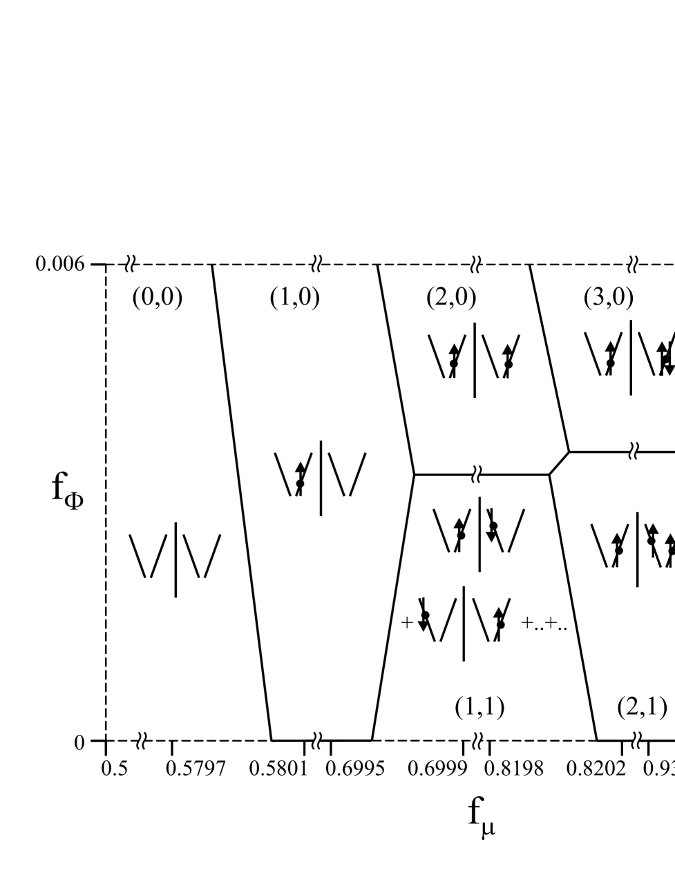
FIG. 2.: The fine structure of the ground state for TNT with $p=0$. The numbers $M_{+},M_{-}$ of right- and left-movers are given in brackets. The parameters $\Delta V(0),{V}_{\pm}(2K)$ are listed in the text below Eq. (18), $K_{++}=0.2$, and $\tilde{a}=1/K$. Quantum states in a coherent superposition are denoted by double dots.

both the spin and orbital configurations are changed. The reconstruction is observable as a jump of the persistent current due to the change in numbers of right and left movers. The increase of the kinetic energy of new ground states is accompanied by the build-up of many-electron correlations, which minimizes the total energy.

For the states $(2,0)$, $(2,1)$, and $(2,2)$ in Fig. 2 the electron spins are parallel, which is a signature of the exchange interaction. The non-diagonal terms (12), (15) of the Hamiltonian do not mix degenerate electron configurations corresponding to each of these states. Let us note that the spin aligned ground states have been presumably detected in very recent experiments [4] on individual linear SWNTs, albeit the data differs substantially from the results [5] on ropes of SWNTs.

The situation is different for the ground states $(1,1)$ and $(3,1)$ (Fig. 2). Each state represents a coherent superposition of $4$ configurations with antiparallel spins, which has the lowest energy due to the interbranch electronic exchange allowed by the non-diagonal matrix elements (12), (15) of the Hamiltonian. The new ground states $(1,1)$, $(2,2)$ with even number of electrons are stable with respect to a change of sign of the magnetic flux. For this reason, TNTs are diamagnetic for even $N_{tot}$ and paramagnetic for odd $N_{tot}$, in contrast to the result of the constant interaction model.

In conclusion, we have generalized the bosonization formalism for the case of TNTs and evaluated the persistent current in this system away from half-filling. The pattern of the persistent current depends on the number of elementary cells along the nanotube modulo 3. The overall pattern (Fig. 1) corresponds to the constant interaction model, whereas the fine structure (Fig. 2) can be explained in terms of electronic exchange correlations. Even though a system with a fixed electro-chemical potential was considered, the results for fixed number of particles can be easily obtained from Eq. (10) and Figs. 1, 2 by an appropriate choice of the electro-chemical potential. A submicroamp persistent current should be observable in a few micrometer long TNTs. The Umklapp scattering of electrons on the atomic lattice (at half-filling), impurities, structural imperfections, twiston phonons, etc. may suppress the persistent current and deserves further analysis.

We would like to thank G.E.W. Bauer, C. Dekker, Yu.V. Nazarov, and U. Weiss for useful discussions. The financial support of FOM is gratefully acknowledged. This work is also a part of INTAS-RFBR 95-1305. One of us (A.O.) acknowledges the kind hospitality at the University of Stuttgart.

REFERENCES

[1] A. Thess, et. al., Science 273, 483 (1996).
[2] S.J. Tans, et.al. Nature 386, 474 (1997).
[3] M. Bockrath, et.al. , Science 275, 1922 (1997).
[4] S.J. Tans, M.H. Devoret, R.J.A. Groeneveld, and C. Dekker,
submitted to Nature.
[5] D.H. Cobden, M. Bockrath, P.L. McEuen, A.G. Rinzler, and
R.E. Smalley, preprint cond-mat/9804154.
[6] Yu.A. Krotov, D.-H. Lee, and S.G. Louie, Phys. Rev. Lett.
78, 4245 (1997).
[7] R. Egger and A.O. Gogolin, Phys. Rev. Lett. 79, 5082
(1997).
[8] C. Kane, L. Balents, and M.P.A. Fisher, Phys. Rev. Lett.
79, 5086 (1997).
[9] H. Yoshioka and A.A. Odintsov, preprint cond-mat/9805106.
[10] J. Liu, et. al., Nature 385, 780 (1997).
[11] R.C. Haddon, Nature, 388, 31 (1997).
[12] M.F. Lin, D.S. Chuu, Phys. Rev. B 57, 6731 (1998).
[13] A.O. Gogolin, A.A. Nersesyan, and A.M. Tsvelik, Bosonization, Cambridge, University Press, 1997.
[14] D. Loss, Phys. Rev. Lett. 69, 343 (1992); D.
Schmeltzer, Phys. Rev. B 47, 7591 (1993); T. Giamarchi, B. Shastry,
Phys. Rev. B 51, 10915 (1995).
[15] Drawbacks of the analysis [7] are discussed
in Ref. [9]
[16] This follows from our definition of (see
inset of Fig. 1a): filling of eight single-particle states at (near) the
crossing points of the spectrum corresponds to , whereas .
[17] D. Mailly, C. Chapelier, and A. Benoit, Phys. Rev. Lett.
70, 2020 (1993).
[18] J.M. Kinaret, M. Jonson, R.I. Shekhter, S. Eggert, Phys.
Rev. B 57, 3777 (1998).
[19] More precise condition, , can
be obtained from the analysis of the strong coupling point where excitations
are gapful. Using the estimate for the (maximum) gap[7], we obtain eV for (10,10) SWNT.