Influence of the temperature on the depinning transition of driven interfaces

Abstract

We study the dynamics of a driven interface in a two-dimensional random-field Ising model close to the depinning transition at small but finite temperatures $T$ using Glauber dynamics. A square lattice is considered with an interface initially in (11)-direction. The drift velocity $v$ is analyzed using finite size scaling at $T=0$ and additionally finite temperature scaling close to the depinning transition. In both cases a perfect data collapse is obtained from which we deduce $\beta\approx 1/3$ for the exponent which determines the dependence of $v$ on the driving field, $\nu\approx 1$ for the exponent of the correlation length and $\delta\approx 5$ for the exponent which determines the dependence of $v$ on $T$.

PACS: 68.35.Rh, 75.10.Hk, 75.40.Mg

The motion of a driven interface in a random medium has attracted a large amount of interest recently because it is a challenging theoretical problem and because it occurs in many different areas of physics like fluid invasion of porous media [3], depinning of charge density waves [4] or field driven motion of a domain wall in a ferromagnet [5], to name just a few. In these cases the disorder is time independent or quenched. For zero temperature there is a well defined critical driving force $F_{c}$ above which the interface moves while the interface gets trapped in metastable positions below it. This scenario has been observed in a variety of different works in the past [6].

At finite temperature the depinning transition is smeared out and the interface can move also below $F_{c}$. For very small driving forces a creep motion is expected which is governed by thermal activation while for driving forces close to the critical one a scaling behavior of the interface velocity $v$ is expected to occur for small enough temperatures (see [4] where the influence of the temperature on the velocity of sliding charge-density waves is discussed).

The dynamics and the morphology of interfaces in systems with quenched disorder have been investigated in the past within a variety of different models. Most studies focus on equations of motion for the interface itself. Famous approaches are the Edwards-Wilkinson (EW) equation [7] or the Kardar-Parisi-Zhang (KPZ) equation [8] which have been studied extensively both with annealed and quenched disorder. A simple example for a disordered medium in which the motion of an interface can be studied is the random-field Ising model. In this case the interface is a domain wall separating regions of up and down spins. For this system it were Bruinsma and Aeppli [5] who argued with the assumption that the interface can be treated as an elastic membrane that its equation of motion at the depinning transition can be described by the EW equation with quenched disorder. Their arguments are plausible but far from rigorous. Therefore, it is also of great interest to tackle the full problem, i. e. to study the dynamics associated with the Hamiltonian of the random-field Ising model prepared initially with an interface. Under the influence of external forces the domain wall may begin to move in a way which depends on the strength of the disorder. A still unsolved problem is the scaling behavior of the velocity of the domain wall for small but finite temperature close to the critical driving field. This, of course, is an important issue also experimentally [9].

It is the purpose of this letter to elucidate this critical behavior of a domain wall in a two-dimensional random-field Ising model close to the pinning transition. Finite size scaling is used for the analysis of the zero temperature behavior resulting in precise values of the exponents. For the first time we determine the critical exponent $\delta$ associated with the finite temperature smearing of the transition which to the best of our knowledge is unknown at present.

For a random-field Ising system in previous work [10] a cubic structure was considered with an interface between up and down spins initially parallel to one of the cubic axis of the lattice. An applied magnetic field $H$ favoring the up spins energetically leaves the down spins in a metastable state. Under the influence of some dynamical rules the area occupied by metastable states shrinks, i. e. the interface starts to move. For the dynamics at zero temperature simple relaxation dynamics was assumed, i. e. a spin is flipped only if its energy is lowered. Additionally it was assumed that only spins at the interface are allowed to flip in order to avoid spontaneous domain growth in the metastable state. The critical field was approached from below, i. e. the driving field was increased in small steps until the pattern of flipped spins after an increase of the field spans the system. The field value for this to happen is the critical field $H_{c}$ .

The geometry used in these investigations has the disadvantage that even without impurities the interface is pinned for up to quite large fields. For space dimension $d=2$, for instance, the driving field has to be larger than $2J$ for the interface to move where $J$ denotes the nearest neighbor exchange interaction. But if one spin of the interface is flipped all neighbors in the same line will flip in the following updates. Thus for zero or very small disorder the movement of the interface consists of a series of complete lines of spins which flip resulting in faceted growth. In this case pinning of the interface is not due to disorder but to the fact that any spin in the interface is locked by its four neighbors. Faceted growth can occur in any dimension for weak and bounded disorder but it depends on the structure of the lattice [11].

By changing the geometry, i. e. considering a (11)-interface instead, it is possible to have an interface which without disorder moves for arbitrarily small driving fields. The dynamics of the interface is then well defined for any strength of the disorder. However the most important observation is that now the conventional $T=0$ dynamics in which a spin flips if this lowers the energy of the system can be generalized to finite temperatures. Since for weak disorder only small driving fields are needed at low temperatures conventional Glauber dynamics can be used without running into the problem of spontaneous domain growth in the metastable phase. For small, bounded disorder there occurs a separation of time scales in the sense that for the system considered within the necessary simulation time only interface motion is observed. The time scale for which the system runs into thermal equilibrium - which Glauber dynamics necessarily does of course - is many orders of magnitude larger, for more details see below. This clear separation of time scales makes a numerical study of temperature effects close to the pinning transition feasible.

The random-field Ising model we consider is defined by the Hamiltonian

$${\cal H}=-J\sum_{<ij>}\sigma_{i}\sigma_{j}-H\sum_{i}\sigma_{i}-\sum_{i}H_{i}\sigma_{i},$$ (1)

where $\sigma_{i}=\pm 1$ are Ising spins on a two dimensional lattice. The first sum describes the ferromagnetic nearest neighbor interaction ($J>0$). The random fields $H_{i}$ are taken from a distribution which is constant within an interval $[-\Delta:\Delta]$ and hence are bounded. $H$ is the homogenous driving field.

The lattice we consider is shown in Fig. 1a). It has the structure of a square lattice but it is rotated by an angle of $\pi/4$. Hence, the boundaries and the initially flat interface of the system are in (11)-direction. We use periodic boundary conditions parallel to the interface. Therefore all spins at the initial interface have exactly two of its four nearest-neighbor bonds broken, i. e. it does not cost any exchange energy to flip a spin at the interface. Hence, without disorder there is no pinning of the interface.

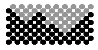
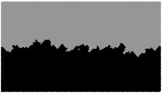
FIG. 1.: a) (upper picture) Schematic picture of a domain wall in the simulated lattice configuration. b) (lower picture) Domain wall of a simulated system of size $100\times 100$ at the depinning field ($H_{c}=1.29J$) for finite temperature ($T=0.1J$).

In the direction perpendicular to the interface we use fixed boundary conditions. Spins in the lowest line are always up (in direction of the driving field) and in the last line are always down. At the beginning of the simulation all spins except of the lowest line are down and, hence, the interface is above the first line. Later, during the simulation the interface moves up due to the driving field.

For finite temperature we perform Monte Carlo simulations where the spins are updated randomly using a heat-bath algorithm. For zero temperature this algorithm naturally crosses over to an algorithm where spins are only flipped when its energy decreases when flipped.

Fig. 1b) shows a system of size $100\times 100$ spins during the simulation. The strength of the random field is $\Delta=1.5J$ and we will use this value throughout the whole paper. The driving field is $H=1.29J$. We will show later that this value is the critical depinning field for $\Delta=1.5J$ at zero temperature. The interface seen is not pinned due to a finite temperature of $T=0.1J$ used in this simulation. No thermal fluctuation or domains appear in the unstable phase (upper part). This is important for the following reasons. In equilibrium the two dimensional random-field system has no long range ordered phase [12]. Since Monte Carlo simulation in principal leads to equilibrium properties one could expect that the system splits into domains spontaneously so that the concept of a single domain wall within the system is no longer useful. But this is not the case due to a separation of time scales mentioned above. Within the single spin flip method the growth of a domain must start with flipping one spin. The minimum energy needed for this process is $\Delta E=2(4J-H-\Delta)$ which is $3.42J$ here for the critical driving field. The corresponding flipping probability within a Monte Carlo simulation is $\exp(-\Delta E/T)\approx 7\times 10^{-14}$ for $T=0.1J$. Therefore, a thermal fluctuation within the bulk is far from being possible within our simulation time which is less than $10^{5}$ Monte Carlo steps per spin (MCS) – it happens on much larger time scales. Hence, as long as we restrict ourselves to low enough temperatures we can perform simulations without the possibility of spontaneous domain growth in the metastable phase.

The velocity of the domain wall we define as the time derivative of the magnetization in a steady state. Note that at the beginning of the simulation the wall is flat and consequently the system is not in a steady state. In the steady state the magnetization grows linearly with time with fluctuations from sample to sample, of course. The velocity is obtained as averaged slope in this linear region. We average the velocity over many systems (10-160, depending on system size and how close the value of the driving field is to the critical one) and perform simulations for different system sizes ($24\times 400\ldots 400\times 400$) in order to investigate finite size effects systematically.

FIG. 2.: $v$ versus $H$ for $T=0$ and for finite temperatures ranging from 0.01$J$ to 0.16$J$. The system size is $400\times 400$.

Our results for the domain wall velocity $v$ versus driving field are shown in Fig. 2 for different finite temperatures and $T=0$. During this simulation we consider for each temperature only driving fields which are large enough so that the wall crosses the system within roughly

FIG. 3.: $v$ versus $H-H_{c}$ with $H_{c}=1.29J$ determined from finite size scaling (see Fig. 4). $T=0$.

2000MCS. Otherwise we interrupt the simulation. As Fig. 2 suggests we get a nice depinning transition at $H_{c}\approx 1.29J$ which is smeared out for finite temperatures.

The wall velocity $v$ depends on system size as shown in Fig. 3 for $T=0$. Finite size effects are common at equilibrium phase transitions and there it is known that the most reliable values for the critical exponents are deduced from a finite size scaling analysis. We found that finite size scaling also works in the present case. For zero temperature the wall can be pinned and within these simulations we set the velocity of a single system to zero if the wall did not cross the system within roughly 20000 MCS and we interrupt the simulation when more then one half of the simulated systems have velocity zero. In contrast to the situation at ordinary phase transitions here the effect of finite size is reversed: the smaller the systems are the stronger vanishes the order parameter. We use the finite-size scaling ansatz

$$v(L,H)=L^{-\beta/\nu}\tilde{v}\left((H-H_{c})L^{1/\nu}\right),$$ (2)

where for the scaling function $\tilde{v}$ we demand $\tilde{v}(x)\sim x^{\beta}$ for $x\gg 1$ and — in contrast to ordinary phase transitions — $\tilde{v}(x)=0$ for $x\rightarrow 0$.

FIG. 4.: Finite size scaling plot of Fig. 3.

Fig. 4 demonstrates that the finite size scaling ansatz above works well. Note that the scaling function has the unusual property mentioned above, i. e. it goes to zero for $H\rightarrow H_{c}$. From the finite size scaling we get $H_{c}=1.290J\pm 0.003J$, $\beta=0.35\pm 0.04$, and $\nu=1.0\pm 0.05$. Alternatively, these results for $\beta$ and $H_{c}$ can also be obtained directly from Fig. 3 by fitting those data which do not show finite size effects to a power law $v\sim(H-H_{C})^{\beta}$. The corresponding line is also shown in Fig. 3. Note also, that this value for $\beta$ is in agreement with the earlier result in [13] within the error bars.

In order to analyse the finite temperature effects we first note that for the largest system size we investigated ($400\times 400$) there are no finite size effects for velocities $v$ well above 0.2 as suggested by Fig. 3. For $L=400$ all data points except the one close to 0.2 are on a straight line, i.e. increase as a power law without $L$-corrections. Hence, it is safe to neglect size effects for the finite temperature data in Fig. 2. For the smearing of the transition by temperature we expect a scaling behavior [4]

$$v(H,T)=T^{1/\delta}\tilde{v}\left((H-H_{c})T^{-1/(\beta\delta)}\right).$$ (3)

A corresponding scaling plot of our data is shown in Fig. 5.

FIG. 5.: Scaling plot corresponding to Eq. 3 for the data of Fig. 2.

We obtain a perfect data collapse with the following parameters: $H_{c}=1.290J\pm 0.005J$, $\beta=0.33\pm 0.02$, and $\delta=5.0\pm 0.3$. To the best of our knowledge this is the first work in which the exponent $\delta$ is determined for the system considered. Note that the perfect data collapse observed leads to exponents with only very small statistical errors.

Finite size scaling and finite temperature scaling both give independent values for the critical field $H_{c}$ and for the exponent $\beta$, respectively. It is rather satisfying that in both cases the numerical values agree within the error bars.

As was mentioned in the introduction there are arguments in favor of the conjecture that the motion of a domain wall in a random-field system can be described by the EW equation with quenched disorder[5] at the depinning transition. For this equation the scaling relation $\nu(2-\zeta)=1$ has been derived [14] by a functional renormalization group scheme in $4-\epsilon$-dimensions. This scaling relation has been claimed to be valid to all orders of $\epsilon$ [15]. If we adopt this view we are therefore able to determine the roughness exponent of the random-field system without investigating the morphology of the interface. The value we obtain, $\zeta\approx 1$, agrees with the value obtained from an $\epsilon$-expansion which is also claimed to be exact in all orders of $\epsilon$ [14, 15]. Values of this exponent obtained numerically by integrating the EW equation or an automaton version of it [16] scatter between $0.7$ and $1.25$ [17, 16]. From the scaling relation $\nu(z-\zeta)=\beta$ we get $z\approx 4/3$ for the dynamic exponent which - as well as our result for $\beta$ - is also in agreement with the results of Nattermann et al. [14]. Interestingly, our value for the temperature exponent $\delta$ fulfills the scaling relation $\delta=2+1/\beta$ which has been derived by Tang and Stepanow [18] by an extension of the functional renormalization group scheme mentioned above to finite temperatures. All our findings support that the motion of a domain wall in a random-field system can be described by the EW equation. However, for an interface moving with a finite velocity also KPZ-like non-linearities could become relevant but from our numerical data we cannot extract any conclusions concerning a corresponding crossover of the values of exponents or scaling laws.

To conclude, we investigated the influence of finite temperatures on the depinning transition of a driven [11]-interface by a Monte Carlo simulation of the two dimensional random-field Ising model. We used bounded disorder and low temperatures in which case a clear separation of time scales occurs in the sense that no spontaneous growth of domains in the metastable phase appears. We derived the order parameter exponent $\beta\approx 1/3$ as well as the exponent $\nu\approx 1$ of the correlation length using finite size scaling. The corresponding dynamic exponent $z\approx 4/3$ and roughness exponent $\zeta\approx 1$ are determined via scaling relations. The exponent $\delta$ describing the influence of the temperature on the depinning of the domain wall which was unknown before was determined to be $\delta\approx 5$.

Acknowledgments: The work was supported by the Deutsche Forschungsgemeinschaft through Sonderforschungsbereich 166 and through the Graduiertenkolleg ”Heterogene Systeme”. We also thank T. Nattermann for pointing us to Ref. [18], and S. Stepanow and L. H. Tang for providing their preprint [18] prior to publishing.

REFERENCES

- [1] E-mail: uli@thp.Uni-Duisburg.DE
- [2] E-mail: usadel@thp.Uni-Duisburg.DE
- [3] M. Cieplak and M. O. Robbins, Phys. Rev. Lett. 60, 2042 (1988).
- [4] D. S. Fisher, Phys. Rev. Lett. 50, 1486 (1983); Phys. Rev. B 31, 1396 (1985);
- [5] R. Bruinsma and G. Aeppli, Phys. Rev. Lett. 52, 1547 (1984).
- [6] For a recent Review see Scale Invariance, Interfaces and Non-Equilibrium Dynamics, edited by A. McKane, M. Droz, J. Vannimenus, D. Wolf, NATO ASI Series B: Physics Vol. 344, (Plenum Press, New York, 1995).
- [7] S. F. Edwards and D. R. Wilkinson, Proc. Roy. Soc. London, Ser. A 381, 17 (1982).
- [8] M. Kardar, G. Parisi and Y. -C. Zhang , Phys. Rev. Lett. 56, 889 (1986).
- [9] F. Ladieu, M. Sanquer, and J. P. Bouchaud, Phys. Rev. B 53, 973 (1996); U. Nowak, J. Heimel, T. Kleinefeld, and D. Weller, Phys. Rev. B 56, 8143 (1997); S. Lemerle, J. Ferré, C. Chappert, V. Mathet, T. Giamarchi, and P. Le Doussal, Phys. Rev. Lett. 80, 849 (1998).
- [10] H. Ji and M. O. Robbins, Phys. Rev. A 44, 2538 (1991) and Phys. Rev. B 46, 14519 (1992).
- [11] H. Koiller, H. Ji, and M. O. Robbins, Phys. Rev. B 46,5258 (1992).
- [12] M. Aizenman and J. Wehr, Phys. Rev. Lett. 62, 2503 (1989).
- [13] C. S. Nolle, B. Koiller, N. Martys, and M. O. Robbins, Physica A, 205, 352(1994).
- [14] T. Nattermann, S. Stepanow, L. H. Tang, and H. Leschhorn, J. Phys. II 2, 1483 (1992).
- [15] O. Narayan and D. S. Fisher, Phys. Rev. B 48, 7030 (1993).
- [16] H. Leschhorn, Physica A 195, 324 (1993).
- [17] G. Parisi, Europhys. Lett. 17, 673 (1992); D. Kessler, H. Levine, and Y. Tu, Phys. Rev. A 43, 4551 (1992); M. Dong, M. C. Marchetti, and A. A. Middleton, Phys. Rev. Lett 69, 3539 (1993); S. Gulluccio and Y.-C. Zhang, Phys. Rev. E 51, 1686 (1995); L. A. Nunes Amaral, A. L. Parabasi, H. A. Makse, and H. E. Stanley, Phys. Rev. E 52, 4087 (1995); M. Jost and K. D. Usadel, Physica A 255, 15 (1998).
- [18] L. H. Tang and S. Stepanow, unpublished; T. Nattermann, March meeting of the American Physical Society (1993)