The Double-Time Green’s Function Approach to the Two-Dimensional Heisenberg Antiferromagnet with Broken Bonds

Abstract

We improved the decoupling approximation of the double-time Green’s function theory, and applied it to study the spin-${1\over 2}$ two-dimensional antiferromagnetic Heisenberg model with broken bonds at finite temperature. Our decoupling approximation is applicable to the spin systems with spatial inhomogeneity, introduced by the local defects, over the whole temperature region. At low temperatures, we observed that the quantum fluctuation is reduced in the neighborhood of broken bond, which is in agreement with previous theoretical expectations. At high temperatures our results showed that the quantum fluctuation close to the broken bond is enhanced. For the two parallel broken bonds cases, we found that there exists a repulsive interaction between the two parallel broken bonds at low temperatures.

]

I Introduction

In recent years, the two-dimensional (2D) antiferromagnetic (AF) spin system on a square lattice has been one of the subjects of major interest in condensed matter physics [3]. This follows from the experiments that copper oxide sheets in the high-T_C superconductors show strong AF correlations [4]. The undoped copper oxide materials are layered AF insulators and well described by the 2D AF Heisenberg model [3]. Doping holes into these materials leads to frustration of spins and ultimately to destruction of AF long-range order (LRO). In the extreme limit of static hole, holes act as local defects and the inhomogeneous Heisenberg model is believed to describe some of the physics [5].

Several numerical and analytical works have been devoted to the effects of isolate defects, e.g., static vacancies [6, 7, 8], broken or ferromagnetic bonds [9, 10, 11, 12], and dynamic holes [13], on the magnetic properties of the 2D antiferromagnet. The inhomogeneous Heisenberg systems are mainly divided into two types. One is the site-defect (SD) model and the other one is the bond-defect (BD) model. These models are important for many fundamental problems, such as frustration, phase separation, and spin glass. Here we adopt the BD model to study the effects of broken bonds replacing AF links in the spin-${1\over 2}$ Heisenberg model at finite temperature. For zero temperature, Lee and Schlottmann have studied this model using the linear spin wave (LSW) theory [9]. They observed that the quantum fluctuation is reduced in the neighborhood of the impurity link and the local magnetic moment is enhanced, in agreement with results obtained by Bulut $et$ $al$ for static vacancy case [6].

At any finite temperature, Mermin and Wagner [14] have proved that for models such as the AF Heisenberg model the AF LRO is destroyed by strong thermal fluctuations in low dimensional systems. Spin wave theory which is based on the existence of LRO can not be directly used at finite temperature. Alternatively, Kondo and Yamaji [15] proposed a second-order Green’s function (SOGF) theory to study the low dimensional Heisenberg model over the whole temperature region. At high temperatures, this theory reproduces the correct results obtained by the high temperature expansion method [16]. On the other hand, the results at low temperatures are similar to those of the modified spin-wave theory [17]. The SOGF theory does not violate the sum rule and rotation symmetry of spin correlations. In the SOGF theory, the decoupling approximation is at a stage one step further than Tyablikov’s random-phase approximation (RPA) [18]. The SOGF theory has been successfully applied to various low dimensional homogeneous systems without LRO, such as the one-dimensional (1D) Heisenberg model [15], the 1D XXZ model [19], the 2D Heisenberg model [20] and the 2D XXZ model [21]. Their results are in qualitative agreement with those numerical results [22, 23] over the whole temperature region.

In this paper we extend the SOGF theory to study the inhomogeneous Heisenberg model by improving the decoupling approximation. The decoupling approximation proposed by Kondo and Yamaji (KYDA) [15] can not be directly applied to the inhomogeneous case without modification. In order not to violate the sum rule in the inhomogeneous case, we introduce an improved decoupling approximation, which is equivalent to the KYDA in the homogeneous case. In our approximation two parameters $\beta_{i}$ and $\beta_{j}$ are attached to the correlation function of the two corresponding spins on sites $i$ and $j$ as $\beta_{i}\langle S_{i}^{+}S_{j}^{-}\rangle\beta_{j}$. While in the KYDA, only one parameter $\alpha_{i}$ is introduced. It is clear that these two parameters account for vertex correction of spin-spin correlation and have to be introduced in order not to violate the sum rule of correlation functions. Thus, in our decoupling scheme, $N$ vertex correction parameters ($\beta_{i}$) for a lattice of $N$ sites were introduced and no other extra parameter. In the homogeneous case, we obtain $\beta^{2}=\alpha$ and our decoupling approximation reduces to the KYDA. Applying this method to the spin-${1\over 2}$ 2D antiferromagnetic Heisenberg model with broken bonds, we obtain reasonable results over the whole temperature region.

The present paper is organized as follow: in Sec. II we present our extension of the SOGF theory to the inhomogeneous spin systems and discuss the improved decoupling scheme. Our numerical results for some particular configurations of one, two, and three broken bond cases are studied in Sec. III. Finally, we conclude our findings in Sec. IV.

II Equation of Motion and Decoupling Approximation

The 2D spin-$\frac{1}{2}$ Heisenberg model with bond-dependent exchange constants can be expressed by the Hamiltonian

$$H=\sum_{\langle ij\rangle}J_{ij}\{\frac{1}{2}(S_{i}^{+}S_{j}^{-}+S_{i}^{-}S_{j}^{+})+S_{i}^{z}S_{j}^{z}\},$$ (1)

where $\langle ij\rangle$ denotes a sum over nearest-neighbor (NN) bonds, and $J_{ij}$ is the exchange interaction between spins on sites $i$ and $j$. For the homogeneous case, $J_{ij}$ is equal to $J$ for all bonds. For the inhomogeneous case we are studying here, $J_{ij}$ equals to zero for broken bond, while it equals to $J$ for unbroken bonds.

We define spin Green’s functions $G$ by

$$G(i-j,~{}t-t^{\prime})\equiv\langle\langle S_{i}^{z}(t);~{}S_{j}^{z}(t^{\prime})\rangle\rangle.$$ (2)

After time-Fourier transformation, the equation of motion of the spin Green’s function $G$ can be evaluated as

$$\omega G(i-j,~{}\omega)=\sum_{\eta}J_{i,i+\eta}\langle\langle S_{i}^{+}S_{i+\eta}^{-}-S_{i+\eta}^{+}S_{i}^{-};~{}S_{j}^{z}\rangle\rangle,$$ (3)

with $\eta$=x̂, ŷ. The SOGF appears on the right hand side of Eq.(3). Furthermore, establishing equation of motion of the SOGF, we have

$$\omega \langle\langle S_{i+\eta}^{+}S_{i}^{-}-S_{i+\eta}^{+}S_{i}^{-};~{}S_{j}^{z}\rangle\rangle$$ (4)

$$= 2\langle S_{i}^{+}S_{i+\eta}^{-}\rangle(\delta_{i+\eta,j}-\delta_{i,j})+2J_{i,i+\eta}\langle\langle S_{i}^{z}-S_{i+\eta}^{z};~{}S_{j}^{z}\rangle\rangle$$ (9)

$$+\sum_{\eta^{\prime}\neq\eta}\{2J_{i,i+\eta^{{}^{\prime}}}[\langle\langle(S_{i+\eta^{\prime}}^{+}S_{i+\eta}^{-}+S_{i+\eta^{\prime}}^{-}S_{i+\eta}^{+})S_{i}^{z};~{}S_{j}^{z}\rangle\rangle$$

$$\hskip 21.68121pt-\langle\langle(S_{i}^{+}S_{i+\eta}^{-}+S_{i}^{-}S_{i+\eta}^{+})S_{i+\eta^{\prime}}^{z};~{}S_{j}^{z}\rangle\rangle)]$$

$$+2J_{i+\eta-\eta^{\prime},i+\eta}[\langle\langle(S_{i}^{+}S_{i+\eta}^{-}+S_{i}^{-}S_{i+\eta}^{+})S_{i+\eta-\eta^{\prime}}^{z};~{}S_{j}^{z}\rangle\rangle$$

$$\hskip 21.68121pt+\langle\langle(S_{i}^{+}S_{i+\eta-\eta^{\prime}}^{-}-S_{i}^{-}S_{i+\eta-\eta^{\prime}}^{+})S_{i+\eta}^{z};~{}S_{j}^{z}\rangle\rangle]\},$$

and the third-order Green’s functions appear on the right-hand side of Eq. (4).

In the homogeneous case, Kondo and Yamaji decoupled the chain of equation (4) in an approximate way [15], for example

$$\langle\langle S_{m}^{+}S_{n}^{-}S_{i}^{z};~{}S_{j}^{z}\rangle\rangle\rightarrow\alpha\langle S_{m}^{+}S_{n}^{-}\rangle\langle\langle S_{i}^{z};~{}S_{j}^{z}\rangle\rangle$$ (11)

for $i\neq m\neq n$. The parameter $\alpha$ was introduced in order not to violate the sum rule of correlation functions. For the inhomogeneous case, the lattice translational invariance does not exist and one needs to introduce $N$ such parameters for a lattice of $N$ sites. However, simply replacing $\alpha$ by $\alpha_{i}$ leads to difficulty in solving self-consistent equations of $G$. Instead, we introduce $N$ parameters $\beta_{m}$ for each site $m$ according to the following relations:

$$S_{m}^{+} = S_{m}^{+}[\beta_{m}-2(1-\beta_{m})S_{m}^{z}]$$ (12)

$$S_{m}^{-} = [\beta_{m}-2(1-\beta_{m})S_{m}^{z}]S_{m}^{-}$$ (13)

for the spin$=\frac{1}{2}$ case. The decoupling approximation for the inhomogeneous systems is thus expressed as

$$\langle\langle S_{m}^{+}S_{n}^{-}S_{i}^{z};~{}S_{j}^{z}\rangle\rangle = \langle\langle S_{m}^{+}[\beta_{m}-2(1-\beta_{m})S_{m}^{z}]$$ (15)

$$[\beta_{n}-2(1-\beta_{n})S_{n}^{z}]S_{n}^{-};~{}S_{j}^{z}\rangle\rangle$$

$$\rightarrow \beta_{m}\langle S_{m}^{+}S_{n}^{-}\rangle\beta_{n}\langle\langle S_{i}^{z};~{}S_{j}^{z}\rangle\rangle.$$ (16)

Here we only keep terms of the lowest order (three operators) Green’s function. On the right hand side of Eq. (7) two parameters $\beta_{m}$ and $\beta_{n}$ are attached to the correlation function of the two corresponding spins on sites $m$ and $n$. It is clear that these parameters are vertex corrections of the spin-spin correlations. According to the definition, we introduce one vertex parameter for each site, and no other extra parameters. In the uniform case we obtain $\beta^{2}=\alpha$, and our decoupling approximation is the same as the KYDA (as shown in Eq. (5)).

With the help of the above decoupling scheme, we obtain the equations of motion of the spin Green’s function $G$

$$\omega^{2}G(i-j,\omega) = \sum_{\eta}2J_{i,i++\eta}\{C(i,i+\eta)(\delta_{i+\eta,\ j}-\delta_{i,\ j})$$ (18)

$$+\langle\langle 2J_{i,i+\eta}(S_{i}^{z}-S_{i+\eta}^{z})+\Pi;\ S_{j}^{z}\rangle\rangle\},$$

where

$$\Pi = \sum_{\eta\neq\eta^{\prime}}\{2J_{i,i+\eta^{\prime}}[\beta_{i+\eta^{\prime}}\beta_{i+\eta}C(i+\eta,i+\eta^{\prime})S_{i}^{z}$$ (22)

$$\hskip 36.135pt-\beta_{i}\beta_{i+\eta}C(i+\eta,i)S_{i+\eta^{\prime}}^{z}]$$

$$\quad\;+2J_{i+\eta-\eta^{\prime},i+\eta}[\beta_{i+\eta}\beta_{i}C(i+\eta,i)S_{i+\eta-\eta^{\prime}}^{z}$$

$$\hskip 36.135pt-\beta_{i+\eta-\eta^{\prime}}\beta_{i}C(i+\eta-\eta^{\prime},i)S_{i+\eta}^{z})]\}~{},$$

here the relation $C(i,j)=\langle S_{i}^{+}S_{j}^{-}\rangle=2\langle S_{i}^{z}S_{j}^{z}\rangle$ has been used.

Since there exists no translational invariance, we can only solve this set of equations of Green’s function in real space. For a finite lattice, the Green’s function $G$ can be expressed in a matrix form $\widetilde{G}$, and Eq. (8) can be rewritten as

$$\omega^{2}\widetilde{G}-\widetilde{h}\ \widetilde{G}=\widetilde{C},$$ (23)

where matrices $\widetilde{h}\$ and $\widetilde{C}$ are made of the nearest-neighbor, the second nearest-neighbor, and the third nearest-neighbor spin-spin correlation functions. We solve self-consistent equation (10) to determine the spin-spin correlation functions and the vertex correction parameters $\beta_{i}$ for each site so to calculate thermodynamical quantities at any temperature.

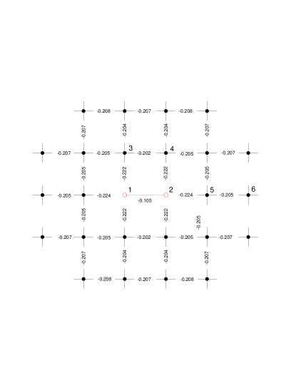
FIG. 1.: The NN correlation functions of the 8$\times 8$ lattice with one broken bond at temperature $T=0.01(2J)$. The dotted line between site 1 and 2 (open circles) represents the broken bond.

III Numerical Results

We have performed numerical calculation on the 6$\times$6, 8$\times$8, and 10$\times$10 lattices with periodic boundary conditions. For the convenience of comparison, we first study the 6$\times$6, 8$\times$8, and 10$\times 10$ homogeneous Heisenberg antiferromagnet. Our results of these finite lattices are quite close to the results of an infinite lattice [20], since the interaction is short-ranged. For the ground state we obtained that the NN correlation function $C_{1}$ is equal to -0.2080 for 6$\times$6 lattice, which is quite close to the corresponding result $-0.2067$ for the infinite lattice [20]. We also studied the staggered structure factor $S(Q)$ ($Q=(\pi,\pi)$ is the AF momentum), defined by,

$$S(Q)=\frac{1}{N^{2}}\sum_{i_{x},i_{y}}\langle[(-1)^{i_{x}+i_{y}}S^{z}(i_{x},i_{y})]^{2}\rangle~{},$$ (24)

and found that its leading finite-size dependence is of order $1/L$, which agrees with the scaling law proposed by other theories [24, 25]. The extrapolated estimate of the staggered magnetization for an infinite lattice is $m=\lim_{L\rightarrow\infty}\sqrt{S(Q)}=0.23$, which grossly agrees with the results of the other theories [24, 25]. Even though we are limited to finite size clusters, our calculation can give reasonable estimates for the infinite system for problems we are interested in.

Let us study the one broken bond case. All configurations of one broken bonds are equivalent within the periodic boundary conditions. Our numerical results of the NN correlation functions near the broken bond for the 8$\times$8 lattice at temperature $T=0.01(2J)$ are shown in Fig. 1. Our results show that the broken bond enhance correlation between spins close to it, which means that the quantum fluctuation close to the broken bond is reduced. The biggest NN correlation function is $C(2,5)=-0.224$, which is about $8\%$ lower than $C_{1}=-0.207$ of the uniform case. At zero temperature, Lee and Schlottmann [9] have studied this model by using the LSW theory. They showed that the quantum fluctuation is reduced in the neighborhood of the impurity link and the local magnetic moment is enhanced. Our results agree with the results of the LSW theory.

The scaling effect of the NN correlation functions close to the broken bond is shown in Table I. We found that the results of the $8\times 8$ lattice are very close to that of the 10$\times$10 lattice. We also found that the NN correlation functions in the next neighborhood of the broken bond are reduced, that is, the quantum fluctuation gets enhanced as the distance to the broken bond increases.

TABLE I. The scaling effect of the NN correlation functions of some special NN sites (labeled as in Fig. 1). The NN correlation function of uniform case is $C_{1}=-0.207$.

$N\times N$	$C(1,2)$	$C(3,4)$	$C(2,5)$	$C(5,6)$
6$\times$ 6	-0.114	-0.200	-0.226	-0.204
8$\times$ 8	-0.105	-0.202	-0.224	-0.205
10$\times$ 10	-0.101	-0.203	-0.224	-0.205

The energy cost for removing one bond from the homogeneous lattice is defined as

$$\Delta_{1}=E^{1}_{0}-E^{0}_{0},$$ (25)

where $E^{0}_{0}$ is the ground state energy of the uniform case, and $E^{1}_{0}$ is the ground state energy of the one broken bond case. For the 8$\times$8 lattice, we obtained that $\Delta_{1}=0.10(2J)$, which is smaller than the energy per bond $\frac{E^{0}_{0}}{2N}=-0.312(2J)$ of the 8$\times$8 homogeneous Heisenberg model. This different is due to the fact that the magnetic system has lowered its energy considerably by readjustment of its spin correlations.

FIG. 2.: The temperature dependent of the NN correlation functions $C(2,5)$ (solid line), $C(5,6)$ (dashed line) and $C(3,4)$ (dash-dotted line) of 8$\times$8 lattice. The dotted line is the result of the homogeneous model.

The temperature dependent of $C(2,5)$, $C(5,6)$ and $C(3,4)$ are shown in Fig. 2. For the convenience of comparison, the temperature dependent of NN correlation

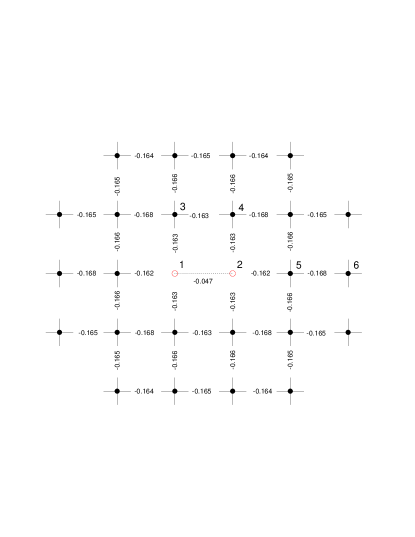
FIG. 3.: The NN correlation functions of 8$\times 8$ lattice with one broken bond at temperature $T=1.5(2J)$. The dotted line between site 1 and 2 (open circles) represents the broken bond.

function $C_{1}$ of the homogeneous Heisenberg model is also plotted (dotted line). In the low temperature region, the correlation function $C(2,5)$ is larger than $C_{1}$. When the temperature increases, $C(2,5)$ drops very quickly and becomes smaller than $C_{1}$ as $T>1.25(2J)$. For the 8$\times$8 lattice, the NN correlation function near the broken bond at temperature $T=1.5(2J)$ are shown in Fig. 3. The biggest NN correlation function is $C(5,6)=-0.168$, which is only about $1\%$ lower than the NN correlation function of the homogeneous case ($C_{1}=-0.166$). It is obvious that the effect of broken bond on the nearby NN correlation functions in the high temperature region is weeker than that in the low temperature region.

FIG. 4.: Two different configurations of the two broken bonds case. 4(a) the two broken bonds are parallel and adjacent; 4(b) the two broken bonds are still parallel but have a distance of two lattice spacing.

For the two broken bonds case, we mainly consider two configurations as shown in Fig. 4(a) and 4(b). In Fig. 4(a), the two broken bonds are parallel and adjacent. While in Fig. 4(b) the two broken bonds are still parallel but the distance between these two bonds increases to two lattice spacing. We obtained that the energy cost of constructing the configuration 4(a) from the homogeneous lattice, e.g., removing two adjacent AF bonds, is $\Delta_{2a}=0.31(2J)$, which is higher than the energy of introducing two isolated broken bonds $2\Delta_{1}=0.20(2J)$. In addition, $\Delta_{2a}$ is quite smaller than the two bond energy $2\frac{E^{0}_{0}}{2N}=-0.624(2J)$ of the uniform case. The corresponding energy of the configuration 4(b) is $\Delta_{2b}=0.24(2J)$, which is more closer to $2\Delta_{1}$ than $\Delta_{2a}$. Thus configuration 4(b) has energy lower than that of 4(a). Our results can be interpreted as that there exists effective repulsive interactions between the two parallel broken bonds.

FIG. 5.: The spin staggered structure factor $S(Q)$ as a function of temperature $T$ for the homogeneous lattice (circle), the one broken bond case (square), the two parallel broken bonds as Fig. 4(a) (diamond) and Fig. 4(b) (up triangle), and the three parallel adjacent broken bonds case(inverse triangle).

The spin staggered structure factor $S(Q)$ ($Q=(\pi,\pi))$ as functions of temperature $T$ for the homogeneous lattice and some particular configurations of one, two and three broken bonds cases are plotted in Fig. 5, respectively. The configuration of three broken bonds shown in Fig. 5 is that the three broken bonds are parallel and adjacent. Our results showed that, although the AF correlation functions close to the broken bonds are enhanced, the AF order of the whole system will be suppressed as number of broken bonds increase.

IV Summary

In conclusion, we have extended the second-order Green’s function theory to the inhomogeneous Heisenberg model by improving the decoupling approximation introduced by Kondo and Yamaji. The Kondo and Yamaji’s decoupling approximation can not be directly expanded to the inhomogeneous case. In this paper, we introduced an improved decoupling approximation, which is in accordance with the Kondo and Yamaji’s decoupling approximation in the homogeneous case. In our approximaton two parameters are attached to the correlation function of the two corresponding spins, which are vertex correction of spin-spin correlation and they have to be introduced in order not to violate the sum rule of correlation functions. We have tried the one parameter scheme (Eq. (5)) and met difficulties in getting the self-consistent equation (10) converge. In our decoupling approximation, there are $N$ vertex correction parameters for a lattice of $N$ sites and no other extra parameter was introduced so we did not add one more parameter than the one parameter scheme. Moreover, our decoupling approximation reduces to the Kondo and Yamaji’s in the homogeneous case.

We apply this theory to study the 2D Heisenberg antiferromagnet with broken bonds for all temperatures. At low temperatures, our numerical results showed that the AF nearest-neighbor correlation functions close to the broken bonds are enhanced. That is, the quantum fluctuation is reduced in the neighborhood of the broken bond at low temperatures. Our results are in agreement with the results of other theories. As the distance to the broken bond increases, the NN correlation functions decreases. By contrast, at high temperatures our results showed that the quantum fluctuation close to the broken bond is enhanced. For the two broken bonds case, we found that there exists repulsive interaction between the two parallel neighbor bonds.

REFERENCES

- [1] Permanent address: Department of Physics, Beijing Normal University, Beijing 100875, China.
- [2] Permanent address: Institute of Physics, Chinese Academy of Science, Beijing, China.
- [3] E. Manousakis, Rev. Mod. Phys. 63, 1 (1991).
- [4] A. P. Kampf, Phys. Rep. 249, 219 (1994).
- [5] A. Aharony ., Phys. Rev. Lett. 60, 1330 (1988).
- [6] N. Bulut, D. Hone, D. J. Scalapino, and E. Y. Loh, Phys. Rev. Lett. 62, 2192 (1989).
- [7] N. Nagaosa, Y. Hatsugai and M. Imada, J. Phys. Soc. Jpn. 58, 978 (1989).
- [8] A. W. Sandvik, E. Dagotto and D. E. Scalapino, Phys. Rev. B56, 11701 (1997).
- [9] Kong-Ju-Bock Lee and P. Schlottmann, Phys. Rev. B42, 4426 (1990).
- [10] A. W. Sandvik, and M. Vekic, Phys. Rev. Lett. 74, 1226 (1995).
- [11] R. E. Camley, W. von der Linden, and V. Zevin, Phys. Rev. B40, 119 (1989).
- [12] V. N. Kotov, J. Oitmaa, and O. Sushkov, and M. Vekic, preprint cond-mat/9802025.
- [13] E. Dagotto, Rev. Mod. Phys. 66, 763 (1994), references there in.
- [14] N. D. Mermin and H. Wagner, Phys. Rev. Lett. 22, 1133 (1966).
- [15] J. Kondo and K. Yamaji, Prog. Theor. Phys. 47, 807 (1972).
- [16] G. S. Rushbrooke, G. A. Baker, and P. J. Wood, Phase Transition and Critical Phenomena (Academic, New York, 1974).
- [17] M. Takahashi, Phys. Rev. B40, 2494 (1989).
- [18] S. V. Tyablikov, Methods in the Quantum theory of Magnetism (plenum, New York, 1967).
- [19] W. J. Zhang, J. L. Shen, J. H. Xu and C. S. Ting, Phys. Rev. B 51, 2950 (1995).
- [20] H. Shimahara and S. Takada, J. Phys. Soc. Jpn. 60, 2394 (1991).
- [21] Y. Fukumoto and A. Oguchi, J. Phys. Soc. Jpn. 65, 264 (1996).
- [22] J. C. Bonner and M. E. Fisher, Phys. Rev. 135, A640 (1964).
- [23] Y. Okabe and M. Kikuchi, J. Phys. Soc. Jpn. 57, 4351 (1988).
- [24] A. D. Huse, Phys. Rev. B37, 2380 (1988).
- [25] A. Z. Liu, and E. Manousakis, Phys. Rev. B40, 11437 (1989).