Scaling in the two-component surface growth

Abstract

We studied scaling in kinetic roughening and phase ordering during growth of binary systems using 1+1 dimensional single-step solid-on-solid model with two components interacting via Ising-like interaction with the strength $K$. We found that the model exhibits crossover from the intermediate regime, with effective scaling exponents for kinetic roughening significantly larger than for the ordinary single-step growth model, to asymptotic regime with exponents of the Kardar-Parisi-Zhang class. Crossover time and length are exponentially increasing with $K$. For a given large $K$, scaling with enhanced exponents is valid over many decades. The effective scaling exponents are continuously increasing with $K$. Surface ordering proceeds up to crossover. Average size of surface domains increases during growth with the exponent close to $1/2$, the spin-spin correlation function and the distribution of domains obey scaling with the same exponent.

PACS: 68.35Bs, 68.35.Ct, 75.70Kw

I Introduction

Growth by vapor deposition is an effective process for producing high quality materials. The microscopic mechanisms of growth were intensively studied in the past mainly in the case of homoepitaxial growth [2, 3, 4]. However, a common situation in nature as well as in modern technologies is growth of binary or more component systems. Due to nonequilibrium nature of growth the properties of resulting film can be very different from properties of equilibrium bulk material, e.g., surface alloys which have no bulk analog can be formed or highly anisotropic structures can be prepared. The problem of growth in a system with two or more components is the problem of great practical importance but it is also interesting from the pure statistical-mechanical point of view, because growth process may belong to a new universality class [5, 6] and such system might exhibit a nonequilibrium phase transition between low and high temperature phase.

There are two interfering phenomena in growth of binary systems: kinetic roughening and phase ordering. During growth the initially flat surface is becoming rough. This is called kinetic roughening. It has been found that this process often fulfills the invariance with respect to scaling in both time and length. Let us consider a surface in a $d$-dimensional space given by a single-valued function $h({\bf r},t)$ of a $d^{\prime}$-dimensional ($d$$=$$d^{\prime}$$+$$1$) substrate coordinate ${\bf r}$. The surface roughness is described by the surface width $w(t,L)=\langle\sqrt{\overline{h^{2}}-\overline{h}^{2}}\rangle$, where $t$ is the time, $L$ is a linear size and the bar denotes a spatial average, $\langle...\rangle$ a statistical average. It often obeys dynamical scaling law $w(t,L)$$\propto$$L^{\alpha}f(t/L^{z})$, with the scaling function $f(x)$ fulfills: $f(x)$ $=$ const., $x$$\gg$$1$ and $f(x)$ $\propto$ $x^{\beta}$, $x$$\ll$$1$ ($\beta$$=$$\alpha/z$). Dynamical scaling allows to classify growth processes into dynamical universality classes according to values of exponents $\alpha$ and $z$ (or $\alpha$ and $\beta$) [7, 8]. This scaling has been observed in a wide variety of growth models and many of them belong to the Kardar-Parisi-Zhang (KPZ) universality class [9]. There has been considerable effort in finding different possible universality classes.

On the other side, the process of ordering in ordinary (nongrowing) binary systems can lead to phase separation. In the case of phase separation dynamical scaling exists as well, e. g. in the Ising model at low temperatures [10]. In phase ordering, the characteristic length $D$ is the average size of domains formed by particles of one type. It increases with time as a power law, $D\propto t^{\psi}$. The dynamics can be classified according to values of the exponent $\psi$. Phase ordering is usually a bulk process, however, one can also study ordering induced by growth only on the surface. In this case the evolution of domain size on the surface is of the interest.

On the microscopic level, growth is usually investigated using discrete growth models. Although several growth models for binary systems were introduced in various contexts, e.g. for the study of phase separation during molecular beam epitaxy [11], or growth of binary alloys [12], our understanding of growth of composite systems is still at the beginning. In particular, little is known so far about kinetic roughening in two-component growth models. This problem was probably first considered by Ausloos et al. [5]. They introduced a generalization of the Eden model, coined a magnetic Eden model, which contains two types of particles with the probabilities of growth given by the Ising-like interaction. Ausloos et al. suggested that the magnetic Eden model does not belong to the KPZ universality class. Recently El-Nashar et al. [6] studied kinetic roughening in a ballistic-like two-component growth model with the varying probability for deposition of given type of particle. They observed that the exponent $\beta$ is changing with the varying probability and argued that kinetic roughening no longer follows the KPZ scaling law. Although the phase ordering was apparently present it was not studied in these works.

In this paper we concentrate on the situation where both processes, kinetic roughening as well as phase ordering, are important and affect each other. We investigate scaling in both roughening of the surface and phase ordering. We use the one-dimensional two-component single-step (TCSS) solid-on-solid growth model which we recently introduced [13]. It is particularly convenient for the study of the asymptotic scaling behavior. Here we present results of extensive numerical simulations which complement the preliminary results published elsewhere [13, 14].

The paper is organized as follows. In Sec. II our model and the measured quantities are defined. In Sec. III results of the Monte Carlo simulations are described, Sec. IV contains discussion. Finally, a summary is given in Sec. V.

II Model and measured quantities

A Modeling of two-component growth

There is a large variety of the single-component growth models which can be potentially generalized to the multicomponent case. Moreover, there are different possible ways of generalization. One usually tries to use a model which is as simple as possible and still contains relevant features. Our aim is to find such model for study of scaling during two-component growth.

The commonly used approximation is application of a discrete model with the so-called solid-on-solid (SOS) condition. It means that the surface is described by a single-valued function $h(i)$ taking discrete values. The index $i$ is the horizontal coordinate which labels sites of the substrate. The rates for elementary growth processes depend usually only on values of $h$ in a neighborhood of the initial and, in the case of diffusion, possibly also of the final position of a particle. The situation is more complex for two-component system because the rates of elementary growth processes depend not only on the geometry but also on the local composition. In practice it means that we need to store the composition in an additional data field. Let us denote the type of a particle by a variable $\sigma$ which takes values $+1$ or $-1$. The geometry of the surface in time $t$ is described by the function $h(i,t)$ and the composition of the deposit is represented by the function $\sigma(i,y)$, where two variables $i$ and $y$ are the horizontal and the vertical coordinates of a particle, respectively. The variable $y$ is restricted only to values from 1 to $h(i,t)$.

Storing the composition of the whole deposit is possible only for relatively small sizes of the substrate and not too many monolayers (ML) of deposited particles. When we study the scaling phenomena, where the behavior for very long times (i.e. many ML) is investigated, too much memory would be required. However, when bulk processes can be neglected, it is sufficient to remember only the composition within a certain finite depth under the surface, because deeper layers cannot affect surface growth. The complication is that the depth which should be stored is in general not well defined and in principle it may be unlimited. For example, to describe the rate for a process in which a particle is moving from or to the bottom of a step we need to store the composition in the depth equal to the maximum step size. But it is known that in some models of MBE growth [15] based on an unrestricted SOS model steps of an arbitrary size can be present. Natural solution of this technical obstacle is to use the so-called restricted SOS model in which possible configurations are limited by an additional constraint $|h(i)-h(j)|\leq N$; $i$ and $j$ being nearest neighbors and $N$ a given integer.

B Two-component single-step model

Our model is based on the simplest restricted SOS model which is the so-called single-step solid-on-solid model. The difference of heights between two neighboring sites is restricted to $+1$ or $-1$ only. The advantage of this choice is that if we restrict ourselves to nearest-neighbor interactions between particles then we can define rates for elementary moves of particles using only the composition on the surface. Hence, the rates at any time are given by the surface profile $h(i,t)$ and the composition only on the surface, which is described by the field $\sigma(i,t)$ of the same dimensionality as $h(i,t)$. We call such model the two-component single-step (TCSS) model.

Implemented growth rules depend in general on the physical situation under study. We consider rather simple case which, however, allows to evaluate the effect of ordering on kinetic roughening. As indicated above, we do not allow bulk processes which exchange particles. This is well justified because rates for such processes are usually several orders lower than for processes on the surface. We also do not include surface diffusion. This is a serious restriction from the point of application to epitaxial growth. However, it is well known that the study of scaling in models with the diffusion is very computer power demanding already in the case of one component growth [15] and that it is difficult to obtain results with a good statistics. We rather consider the condensation-evaporation dynamics. Even more, we restrict ourselves here to the pure growth situation. Evaporation can be included but we expect that it will not change the scaling behavior provided the surface is moving, i.e. deposition occurs more frequently than evaporation.

Hence, during the evolution, particles are only added. Due to the single-step constraint a particle can be added only on the site at a local minimum of height, called growth site. Once the position and the type of the particle are selected, they are fixed forever. The probability of adding a particle of type $\sigma$ to a growth site $i$ depends only on its local neighborhood and is controlled by a change of energy of the system after deposition of a new particle. The energy is given by the Ising-like interaction. The probability is proportional to $\exp\left\{-\Delta E(i,\sigma)/k_{B}T\right\}$, where $k_{B}$ is the Boltzmann’s constant, $T$ is temperature and $\Delta E(i,\sigma)$ is the change of energy [16].

We describe explicitly our growth model for simplicity in 1+1 dimensions but it can be straightforwardly generalized to any dimension. Several realizations of the single-step geometry are possible in 1+1 dimensions (Fig. 1)

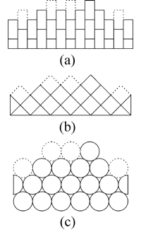
FIG. 1.: Three realizations of the single-step geometry in 1+1 dimensions. Dashed lines indicate positions where a new particle can be deposited.

FIG. 2.: Example of configuration with two types of particles (dark and light gray) in the considered realization of the single-step model. Dashed lines indicate positions where a new particle can be deposited.

leading to three different variants of the TCSS model. They differ in the number of nearest neighbors of a new particle. While in the variant B there is an ambiguity in the type of newly deposited particle if two neighbors are of opposite types, this is not the case in variant A. We expect that the effect of ordering on dynamics is stronger for the variant A than for the variant B. The variant C (Fig. 1c) is technically slightly more complicated to simulate due to the varying number of nearest neighbors of a deposited particle. Therefore, we consider the variant A with three nearest neighbors which is represented as stacking of rectangular blocks with the height equal to double of the width (Fig. 1a). Nevertheless, we expect similar asymptotic scaling behavior for all three variants.

Then expression for the change of energy is

$$\frac{\Delta E(i,\sigma)}{k_{B}T}=-K\sigma[\sigma(i-1)+\sigma(i)+\sigma(i+1)]-H\sigma.$$ (1)

Here, $K$ is a dimensionless coupling strength and $H$ is the bias leading to preferential deposition of particles of a selected type ($+1$ for positive, $-1$ for negative $H$). In analogy with magnetic systems we will call $H$ external field. The sum $\sigma(i-1)+\sigma(i)+\sigma(i+1)$ contains types of particles on the surface within nearest neighbors of the growth site (which are three in the chosen variant: left, bottom and right).

C Measured quantities and simulation procedure

Evolution of the geometry is affected by composition of the surface and vice versa. We characterized the geometry of the surface by the surface width $w(t,L)$ defined in introduction, and by the height-difference correlation function $G\left(r,t\right)=\frac{1}{L}\sum_{i=1}^{L}\langle\left[h\left(i+r,t\right)-h\left(i,t\right)\right]^{2}\rangle$, which is expected to obey a scaling relation [7, 8] $G(r,t)\propto r^{2\alpha}g(r/t^{1/z})$, the scaling function $g(x)$ is constant for $x$$\ll$$1$ and $g(x)$$\propto$$x^{-2\alpha}$ for $x$$\gg$$1$.

In the case of phase ordering we concentrated on evolution of the composition on the surface, which is important for evolution of the geometrical profile of the surface. We measured two quantities defined on the surface: i) the average of surface domain sizes, and ii) the correlation function $S(r,t)$ analogous to spin-spin correlation function used in magnetic systems. We call the surface domain a compact part of the surface, which is composed of particles of the same type. The size of the domain $d$ is measured along the surface. Average size of the surface domains depends on time, on coupling, on external field and also on the initial composition of the substrate. We denote the statistical average of this quantity by $D=\langle d\rangle$. The correlation function $S(r,t)$ is defined as follows: $S(r,t)=\frac{1}{L}\sum_{i=1}^{L}\langle\sigma\left(i+r,t\right)\sigma\left(i,t\right)\rangle$. The only bulk property which we measured was concentration of particles of a given type, $c_{+}$ resp. $c_{-}$ (see subsection III C 4).

We performed simulations for various coupling constant $K>0$ and mostly for zero external field $H$ (except subsec. III C 4). System sizes varied from $L=250$ to $L=80000$, and the number of deposited monolayers (ML) was up to $3\cdot 10^{5}$, but for small systems even up to $4\cdot 10^{6}$ ML. We measured time $t$ of the simulation in the number of monolayers. A statistical average was obtained by averaging over varying number of independent runs. It was from ten (for $L=80000$) up to several thousand (for $L=250$).

The growth starts on a flat surface configuration [17] as usual, but in two-component models the evolution strongly depends on initial composition of the substrate [14]. Here we considered two possibilities i) a neutral substrate, i.e. substrate without any interaction with deposited particles, in this case the system orders spontaneously from beginning, and ii) an alternating substrate, with the alternating types of particles. The case of a homogeneous substrate composed of one type of particles is reported elsewhere [14].

III Results

A Evolution of morphology

Fig. 3 shows examples of time evolution of surface morphologies and compositions for selected couplings and external fields. Note that times for which surface profiles are shown increase exponentially. Visual inspection of many configurations leads to the following observations.

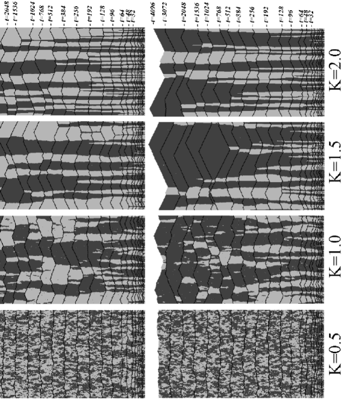
FIG. 3.: Examples of evolution of surface profiles for several values of coupling constant, $K=0.5$, $1.0$, $1.5$, $2.0$, and zero and nonzero external field $h$; (upper panel - $H=0$, lower panel - $H=0.02$). Surface profiles at selected times increasing as powers are indicated by black lines, only part of the grown material close to the surface is shown at given time. Dark and light gray correspond to different types of particles. System size is $L=300$.

In the case of zero external field (upper panel), we can see that with increasing coupling the surface is becoming more and more rough (faceted) and at the same time more and more clean columnar structures are formed; the anisotropy induced by growth is more pronounced. The average width of the columns increases with time. We can also see that, for a given time, average width of the column is decreasing with coupling. This is at the first sight in contradiction with the expectation that ordering should be more pronounced for stronger coupling. Notice also that for larger coupling there is the correlation between the domain walls and the local minima of the surface. Both these effects can by explained from the dynamical rules of the model. We shall discuss this point further in Sec. IV.

The lower panel demonstrates the effect of a small external field. We can see that for small coupling ($K=0.5$) an external field does not cause a significant change of the stoichiometry. The effect of the field is canceled by fluctuations during growth. However, for larger coupling an external field leads to excess of one component. We evaluate this effect quantitatively in subsec. III C 4.

B Kinetic roughening

The original single-step model belongs to the Kardar-Parisi-Zhang universality class [9] with the exponents $\alpha^{(KPZ)}=\frac{1}{2}$, $\beta^{(KPZ)}=\frac{1}{3}$, ($z^{(KPZ)}=\frac{3}{2}$) in 1+1 dimensions. In this subsection we investigate the existence of scaling and the values of scaling exponents for kinetic roughening in the TCSS model.

1 Surface width

We start with the time dependence of the surface width from which we can measure the effective exponent $\beta_{\rm eff}$. In order to avoid the finite size effects caused by the saturation of the surface width we used large system size $L=80000$. We have found that the behavior changes with the strength of coupling. When the coupling is weak, evolution of the roughness is almost the same as in the ordinary single-step model, e.g. for $K=0.3$ the increase of $w(t)$ can be well fitted during all time of the simulation by one power law $w(t)\propto t^{\beta_{\rm eff}}$ with the exponent $\beta_{\rm eff}=0.33$, very close to the KPZ value $\beta^{\rm KPZ}=\frac{1}{3}$ (cf. [13]). For somewhat larger coupling we have observed that the surface width exhibits the crossover in time. At first the width increases with an effective exponent $\beta_{\rm eff}>1/3$, but after certain time $t_{\rm cross}$ it crosses over back to $\beta^{(KPZ)}=\frac{1}{3}$. This can be clearly seen in Fig. 4 (curves for $K=0.7$, $1.0$, and $1.3$) where we plotted the time dependence of the quantity $w(t)/t^{1/3}$ for several couplings in order to compare evolution of the surface width with the KPZ behavior. Notice also that the absolute value of $w$ in a given time is increasing with $K$.

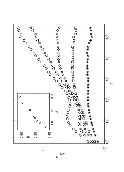
FIG. 4.: Surface width $w$ divided by $t^{\frac{1}{3}}$ vs. time $t$ for several values of coupling constant, $K=$ 0.7 ($\ast$), 1.0 ($\Box$), 1.3 ($\Diamond$), 2.0 ($\triangle$), 3.0 ($\circ$) and zero external field, $L=80000$. Inset: Effective scaling exponent $\beta_{\rm eff}$ before crossover as function of coupling.

The crossover from the regime with the enhanced $\beta_{\rm eff}$ to the regime with $\beta=\frac{1}{3}$ is definitely not a finite size effect. We checked that the time $t_{\rm cross}$ is the same for different system sizes.

From Fig. 4 we can also see that $t_{\rm cross}$ is increasing with coupling. We were not able to observe the crossover to the KPZ behavior for coupling $K\geq 2$ in the time scale of our simulations [18]. In order to estimate the time needed we plotted the dependence of $t_{\rm cross}$ on $K$ (Fig. 5).

FIG. 5.: Crossover time $t_{\rm cross}$ for the crossover in the behavior of the surface roughness ($\Diamond$), saturation time $t_{\rm sat}$ for saturation of the average domain size ($\Box$), saturated value of the average domain size $D_{\rm sat}$ ($\ast$), and saturated value of the correlation length $\xi^{s}_{\rm sat}$ ($\circ$) vs. coupling $K$.

It can be fitted as $t_{\rm cross}(K)\propto e^{8.4K}$. When we extrapolate this data to $K=2$ we get $t_{\rm cross}(K=2)>10^{6}$ which is longer then the time of our simulation.

We found that for any $K>0.7$ there is a time interval extending over several decades in which we can well fit our data as a power law with the exponent $\beta_{\rm eff}>1/3$, before there is crossover to the KPZ behavior or our simulation stops. The question remains, whether $\beta_{\rm eff}$ goes to a specific value for large $K$. We did not find the indication that $\beta_{\rm eff}$ saturates to a certain value, at least for the investigated range of coupling $K\in[0,3]$. The effective exponent $\beta_{\rm eff}$ is increasing function of $K$ (see inset in Fig.4). We attribute the rather large value of $\beta_{\rm eff}$ for strong coupling to pinning of the surface at domains boundaries.

2 Height-difference correlation function

The second exponent for kinetic roughening is the roughness exponent $\alpha$. It can be calculated from the dependence of the saturated surface width on the system size. We used here an alternative and often more accurate way. We calculate $\alpha$ from the spatial dependence of the height-difference correlation function $G\left(r,t\right)\propto r^{2\alpha}$ in the long time limit.

The obtained exponents $\alpha$ also depend on coupling. Exponent $\alpha$ has a value close to $\alpha^{(KPZ)}=\frac{1}{2}$ for weak coupling. For larger coupling, we have found that when the system is sufficiently large there is a crossover behavior in the spatial dependence of the height-difference correlation function (see Fig. 6). On the small length scale it increases faster than $r$, and for sufficiently large $K$ we can fit it as a power law $r^{2\alpha_{\rm eff}}$ with an effective exponent $\alpha_{\rm eff}>\frac{1}{2}$. However, if the distance is larger than certain length $l_{\rm cross}$, the form of the function crosses over to power law with the exponent which is close to $\frac{1}{2}$, i.e. to the KPZ behavior (cf. data for $K=1$ in Fig. 6).

If the coupling is strong $(K\geq 2)$ we do not see the crossover but only the larger exponent $\alpha_{\rm eff}\approx 1$. We expect that it is because even the system size $L=80000$ and time 262144 ML are not large enough to get into the crossover regime. We have found that $\alpha_{\rm eff}$ is increasing smoothly with the strength of coupling from $\alpha^{(KPZ)}=\frac{1}{2}$ to a value slightly less than one (inset in Fig. 6). The value $\alpha=1$ is the natural limit imposed by the single-step constraint.

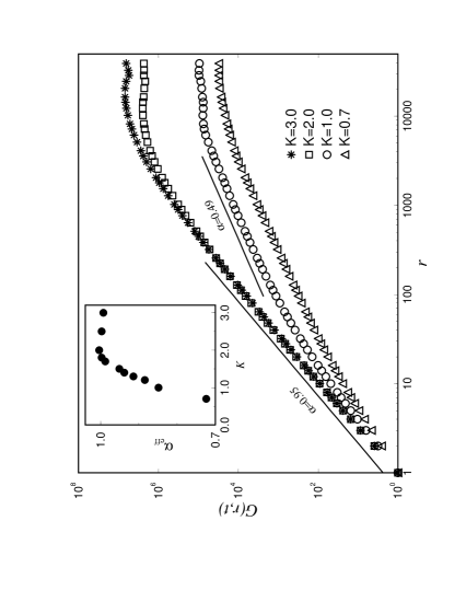
FIG. 6.: The height-difference correlation function $G(r,t)$ for couplings $K=0.7$, $1.0$, $2.0$, and $3.0$ after 262144 ML were deposited, $L=80000$. Inset: Effective exponent $\alpha_{\rm eff}$ before crossover as function of coupling.

FIG. 7.: Data collapse of the correlation function $G(r,t)$ for coupling $K=2$ obtained for exponents $\alpha=0.97$ and $z=1.97$.

3 Scaling

Having both exponents $\alpha$ and $\beta$, we can try to verify scaling. For weak coupling, the exponents are close to the KPZ exponents and scaling with these exponents is satisfied. For larger coupling, when the crossover is observed, we cannot get scaling for all times and lengths, nevertheless for long times and large lengths the KPZ scaling is valid. When coupling is sufficiently strong then the behavior characterized by enhanced exponents extents over many decades of time and length and looks practically as asymptotic. Then we can ask ourselves if there is scaling with new exponents which is satisfied on this scale. In order to show that there is scaling, we should get data collapse. We have found that indeed we get the data collapse over many decades in the strong coupling regime ($K\geq 2$). As an example we show in Fig. 7 the data collapse of the height-difference correlation function $G(r,t)$ obtained for $K=2$ with exponents $\alpha=0.97$ and $z=1.98$. For different $K$ we need different exponents, e.g., for $K=3$ we get the best data collapse for $\alpha=0.99$ and $z=1.7$. The question remains what is true asymptotic scaling in the strong coupling regime. We expect that for any $K$ there is crossover to the KPZ scaling (although $t_{\rm cross}$ may be astronomically large), and the asymptotic behavior will belong to the KPZ class.

C Phase ordering

1 Time evolution of surface domains

Time evolution of the average surface domain size $D$ for several couplings is shown in Fig. 8. We can see that the behavior again depends on $K$. For small coupling, $D$ at first increases, however after some time $t^{(D)}_{\rm sat}(K)$ surface domain size saturates to a value $D_{\rm sat}(K)$. We have checked that the saturation is not a finite size effect (see [13] - inset in Fig. 3). This is an intrinsic property of the model. Both the time $t^{(D)}_{\rm sat}(K)$ and the saturated value $D_{\rm sat}(K)$ rapidly increase with $K$ (Fig. 5). We have found that the dependence on $K$ can be well fitted by exponentials: $D_{\rm sat}(K)\sim{\rm e}^{(2.91\pm 0.06)K}$ and $t^{(D)}_{\rm sat}(K)\sim{\rm e}^{(7.67\pm 0.06)K}$. We were not able to observe saturation for $K=2$ because of prohibitively long simulation time needed. Hence, for $K\geq 2$ the domain size is increasing during all time of our simulation. But we believe that the evolution of the surface domains is analogous to evolution of domains in one-dimensional Ising model and that in long time it will saturate for any $K$ [19].

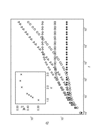
FIG. 8.: Time evolution of average surface domain size for coupling constants $K=$ 0.7 ($\ast$), 1.0 ($\Box$), 1.3 ($\Diamond$), 2.0 ($\triangle$),3.0 ($\circ$) and zero external field, $L=80000$. Inset: Effective exponent $\psi_{\rm eff}$ as function of coupling $K$.

Evolution of domains is strongly affected by initial conditions and a certain transition time is needed before a value independent on the initial state is reached. This phenomenon is similar to what we have observed in the case of surface width. The transition time is increasing with coupling and can be quite long, e.g. for $K=3$ it is several hundred of ML.

We have found that for $K\geq 1$ there is a time interval in which the increase of average domain size can be fitted by a power law, $D(t,K)\propto t^{\psi_{\rm eff}(K)}$ with an exponent $\psi_{\rm eff}$ depending on $K$. For large $K$ the exponent $\psi_{\rm eff}$ seems to saturate to a value slightly smaller than $\frac{1}{2}$ (see inset in Fig. 8). This is the same exponent as for the Ising model with nonconserved order parameter [10].

2 Distribution of surface domain sizes

The average surface domain size contains the information about the formation of the domains during the growth. However, it is not clear only from that quantity, whether the domains form a kind of periodic structure with a typical domain length or the domain sizes are rather random. In order to obtain more information about the domains, we measured the probability distribution $P(d,t)$ of domain sizes $d$ as a function of time. We performed the simulations for three values of coupling $K=1$, $K=2$ and $K=3$, the system size was $L=1000$, and time up to 32768 ML. In order to get good statistics we had to make the average over ten thousand independent runs. We observed that for initial times there is a rather sharp asymmetric peak with the position shifting to higher values of $d$ with increasing time. During time evolution the amplitude of the peak decreases and the peak becomes more and more broad and eventually disappears. The time scale for this behavior depends on $K$.

We try to rescale our data extending over many orders of magnitude and to look if there is scaling. We applied a scaling formula of the form

$$P(d,t)=F(d/D(t))/D(t),$$ (2)

with a scaling function $F$. The average domain size $D(t)$ is in fact equal to the average computed from the distribution $P(d,t)$.

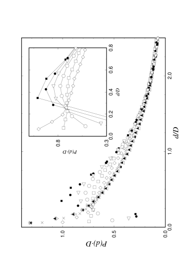
FIG. 9.: Distribution of domain sizes for $K=1$ and times 4 (full square), 8 (full circle), 16 (triangle left), 32 (circle), 64 (square), 128 (diamond), 256 (times), 512 (triangle down), 1024 (plus), 6144 (triangle up), 32768 (full triangle). Inset: Detail of the distribution. The symbols are the same as in the main graph.

In the Fig. 9 the rescaled distribution of domain sizes for $K=1$ is shown as a function of the variable $x=d/D$, for times from 4 to 32768. We can see that the peak at around $x=0.4$ exists only for short times and for time about $t=64$ it changes to a small plateau which further vanishes for longer times. The distribution of domain sizes for long times converges to a function which we found to be well fitted by an exponential. Moreover, we found that the peak vanishes around the time $t^{(D)}_{\rm sat}$ when the average domain size saturates.

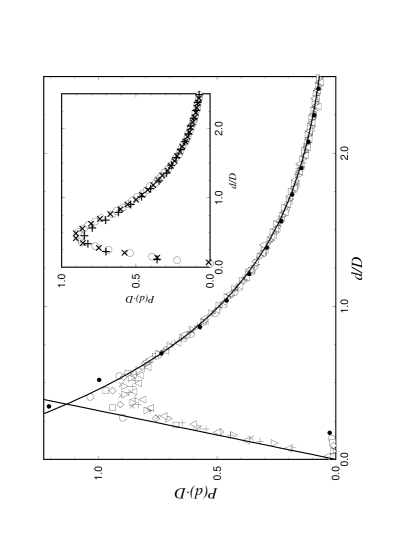
FIG. 10.: Distribution of domain sizes for $K=2$ and times 8 ($\bullet$), 32 ($\circ$), 64 ($\Box$), 128 ($\Diamond$), 256 ($\times$), 512 ($\bigtriangledown$), 1024 (+), 6144 ($\triangle$). The full lines are exact results for the kinetic Ising model, ref. [21], in the limits of small and large $d/D$. Inset: Distribution of domain sizes for $K=1$ in time 16 (+), for $K=2$ in time 256 ($\times$) and for $K=3$ in time 4096 ($\circ$).

The results for $K=2$ are shown in Fig. 10. We can see that the scaling formula (2) is satisfied from the time 8 to 6144. The data for longer times are not shown here because after 10000 independent runs they still have too big noise. The scaling function $F(x)$ has a maximum again near $x=0.4$. This indicates creation of a quasi-regular domain structure, but the distribution has very broad tail for larger $x$ extending up to $x\simeq 4$, which makes the domain structure irregular. We compared the scaling for different $K$. For times shorter than the saturation time the scaling function does not depend on $K$, which is demonstrated in the inset in Fig. 10 for $K=1.0,2.0$, and $3.0$.

The behavior similar to that in the strong coupling regime was observed for the kinetic Ising model in one dimension. Numerical simulations of the Ising model at zero temperature [20] show that the distribution of domain sizes obeys the form (2) with a peak around $d/D\simeq 0.4$. Also the form of the function $F(x)$ found in [20] looks very similar to our results. On the contrary, for any non-zero temperature it may be shown analytically, that the distribution of domain sizes in equilibrium, i.e. in the infinite time limit, is exponential (see e.g. [21]). Analytical results for the zero-temperature kinetic Ising model [22] give the asymptotic results $F(x)\simeq\pi x$ for $x\to 0$ and $F(x)\simeq\exp(-Ax+B)$ for $x\to\infty$, with $A=\frac{1}{2}\zeta(3/2)=1.30618...$, and $B=0.597...$, which is in good agreement with our results, as Fig. 10 shows.

Summing up, we should again distinguish two time regimes. At initial times, the form of the distribution of domain sizes as a function of $x$ does not change and it is characterized by a pronounced peak. Scaling (2) holds and the only change during the time evolution is the increase of the average domain size $D$. When $D$ begins to saturate, the peak vanishes and in the saturated regime, the distribution of domain sizes is exponential. The reason why in the case of strong coupling ($K=2.0,3.0$) the peak remained for all times observed is simply that the duration of the simulation is still much shorter than the saturation time.

3 Correlation function

The correlation function $S(r,t)=\frac{1}{L}\sum_{i=1}^{L}\langle\sigma\left(i+r,t\right)\sigma\left(i,t\right)\rangle$ decays nearly exponentially with the distance $r$. The decay is characterized by the correlation length $\xi^{s}(t,K)$ which we computed by fitting the data to the function $\exp(r/\xi^{s}(t))$ in an interval $(0,r_{s})$ in which the decay is actually well described by an exponential. According to our experience a good recipe for fixing the interval $(0,r_{s})$ is to find the distance $r_{s}(t)$ as the minimal distance for which $S(r_{s}(t),t)\leq 0.05$. This is done for given time and coupling.

The time behavior of the correlation length $\xi^{s}(t,K)$ is similar to that of the average domain size $D(t,K)$. It increases with time as a power law $\xi^{s}(t,K)\propto t^{\kappa_{\rm eff}(K)}$ (we found $\kappa_{\rm eff}\simeq 0.5$ for $K=2$). For weak coupling $K$, $\xi^{s}(t,K)$ saturates to a finite value $\xi^{s}_{\rm sat}$ at about the same time $t^{(D)}_{\rm sat}$ as the saturation of the average surface domain size occurs. The saturation for large $K$’s cannot be seen because the simulation time is insufficient. The dependence of the saturated correlation length $\xi^{s}_{\rm sat}$ on $K$ is shown in Fig. 5. It can be fitted by an exponential, $\xi^{s}_{\rm sat}\simeq{\rm e}^{(3.29\pm 0.03)K}$. This behavior is similar to what was observed for for $D_{\rm sat}$ (cf. Fig. 5).

For times shorter than $t^{(D)}_{\rm sat}$ we observed the following scaling: $S(r,t)=\bar{S}(r/t^{\nu})$, the value of exponent $\nu$ for $K=2$ is $\nu=0.465$ (Fig. 11).

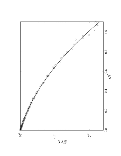
FIG. 11.: Spin-spin correlation function $S(r,t)$ as function of $\frac{r}{t^{\nu}}$ for $K=2$ in times 512 ($\circ$), 1024, ($\Box$), 6144 ($\Diamond$), 32768 ($\times$), 65536 ($\triangle$), 131072 ($+$). The solid line is the fit with function $\exp(-bx-ax^{2})$, $a=2.6$, $b=1.86$, $x=r/t^{\nu}$, $\nu=0.465$.

The function $\bar{S}(x)$ was found to have the form $\bar{S}(x)=\exp(-bx-ax^{2})$ where the parameters $a,b$ were fitted as $a=2.6\pm 0.1$ and $b=1.86\pm 0.09$. This behavior agrees with analytical results for the zero-temperature kinetic Ising model [23]. The correlation functions $S(r,t)$ for time larger than $t^{(D)}_{\rm sat}$ do not depend on time but they depend on $K$. These functions $S_{\rm sat}(r,K)$ can be also scaled into universal form using the saturated correlation length $S_{\rm sat}(r,K)=\tilde{S}(r/\xi^{s}_{\rm sat}(K))$.

4 Concentration of components

We measured also the quantity $m=\frac{1}{L}\sum_{i}\sigma_{i}$, which is an analog of the surface magnetization and from which the concentrations of both components, $c_{+}=\frac{1+m}{2}$, $c_{-}=\frac{1-m}{2}$, on the surface can be determined. In all the simulations described so far the external field was zero, therefore $m$ (after a sufficient averaging) was zero, i.e. average concentration of one component was 50 % and constant in time. However, for nonzero field average $m$ is no longer zero and it depends on time and external field, i.e. there is time dependent excess of one component. When time of the simulation is sufficiently long we arrive to the stationary state with a characteristic value of $m^{\rm stat}(H,K)$ which corresponds to the concentration of both components produced in the stationary regime.

The quantity $m$ can be obtained from our simulations, however, it is the subject of rather strong fluctuations. Instead of $m$ we measured the corresponding bulk quantity $M$. In order to follow the time dependence we measured $M$ in the same time intervals as the surface width, i.e. in the logarithmic scale, but we recorded only sum of $\sigma$’s of particles deposited between two intervals of measurement divided by the total number of particles deposited during this interval. Therefore, $M(t)$ is not the total bulk magnetization but “incremental” bulk magnetization. The numbers of particles deposited in each time interval increase as $L$, $2L$, $4L$, $8L$, $\cdots$. Hence, for a long time we are averaging over many bulk particles and approaching to the total bulk magnetization. The fluctuations of $M(t)$ are smaller than fluctuations of $m(t)$. In all simulations in this subsection we started from the substrate with alternating types of particles, it implies $M(0)=m(0)=0$. We continued the simulations up to time when the stationary regime was reached and we measured $M^{(\rm stat)}(H,K)$. Time needed depends on both $H$ and $K$. From $M^{(\rm stat)}$ we can obtain the stationary concentrations. However, we prefer to use the quantity $M^{(\rm stat)}$ in order to utilize the analogy with magnetic systems.

FIG. 12.: Dependence of stationary bulk magnetization $M^{\rm stat}$ on inverse coupling $\frac{1}{K}$ for several external fields.

In Fig. 12 we plotted $M^{(\rm stat)}(H,K)$ as function of $1/K$ for several values of $H$. When coupling is small the effect of external field is weak and $M^{(\rm stat)}$ is close to zero, i.e. concentration changes very little, and $M^{(\rm stat)}$ is close to the value corresponding to zero coupling [24]. For large $K$, dependence on external field becomes very strong (cf. also Fig. 3).

For $K>1.5$ the magnetization seems to go to a finite limit when external field goes to zero indicating possible existence of the bulk phase transition. However, our present data are for rather small system and more detailed study of finite-size effects is needed in order to decide on the presence or absence of the bulk phase transition.

IV Discussion

The crossover in the surface width as well as in the height-difference correlation function is clearly related to stopping of phase ordering on the surface. We observed that time for saturation of domain $t^{(D)}_{\rm sat}$ is approximately proportional to time $t_{\rm cross}$ for crossover to the KPZ exponent $\beta=1/3$ in evolution of the surface width (Fig. 5). Due to progressively increasing time and system size needed for the simulation we cannot decide from our data whether the crossover is present for any coupling, or if there is a phase transition at a certain critical coupling $K_{c}$, and for $K>K_{c}$ the exponents remain enhanced. However, we do believe that the crossover is present for any value of $K$, but it is hard to see it for strong coupling because $t_{\rm cross}$ is larger than possible simulation time.

In the surface morphology, the most striking features are the pyramids or teeth observed for a sufficiently large coupling $(K\geq 1.5)$. This can be understood from the rules of growth. Let us consider a growth site with all nearest neighbors of the same type. The probability that it will be occupied by a new particle is $\propto(e^{3K}+e^{-3K})$. The first term, $e^{3K}$ gives the probability that a new particle will be of the same type as the old ones. This is much larger than the second term corresponding to the probability that a new particle will be of the opposite type. The creation of new domain walls is thus strongly inhibited and growth proceeds preferably by adding the particles of the same type. On the other hand, probability to occupy a growth site next to the boundary between two domains is $\propto(e^{K}+e^{-K})$, i.e. smaller than the growth probability inside the domain. Hence, growth inside the domain is preferable. This leads to the formation of pyramid-like features composed of one type of particles with facets of maximal slope and domain walls in bottoms of the valleys. In other words growth is pinned by domain walls. This is in accord with the results on non-homogeneous growth, where the presence of the inhomogeneity leads to the formation of a dip in the surface [25, 26].

At the same time, if we observe the deposition of particles next to the domain wall, we can see that the wall movement is due to deposition of opposite type of particle, which has probability $\propto{\rm e}^{-K}$, while no movement has probability $\propto{\rm e}^{K}$. That is why the wall movement is very slow for large $K$. The surface domains with slowly moving walls result in long vertical lamellae (cf. Fig. 3). This leads to at first sight surprising fact that the width of lamellae of different types of particles decreases with coupling (for equal times), which we observed for the growth with initial condition fixed by neutral substrate [27]. This is also reason of longer transient times for larger $K$.

Non zero external field leads to surface (as well as bulk) magnetization, or in the context of alloy growth, to changing stoichiometry. We can still define exponent $\psi$ for growth of the dominant domain size as well as exponents for kinetic roughening. Effect of this symmetry breaking on values of exponents remains to be studied.

V Conclusion

We have investigated the interplay between phase ordering and kinetic roughening using the 1+1 dimensional two-component single-step SOS growth model. We examined validity of scaling for both phenomena and measured the effective scaling exponents.

We observed two situations depending on the strength of coupling $K$ between two types of particles. For a moderate, sufficiently strong ($K>0.3$) but not very large ($K<1.8$) coupling, there is crossover in time and spatial behavior of geometrical characteristics of the surface profile. The effective exponents $\alpha$ and $\beta$ for time shoter than $t_{\rm cross}$ are significantly larger than the KPZ exponents. After crossover we observed the KPZ exponents. Surface ordering proceeds only up to a finite time $t^{D}_{\rm sat}(K)$ after which it stops. Crossover time $t_{\rm cross}$ is proportional to $t^{D}_{\rm sat}(K)$ and both are exponentially increasing with the strength of coupling. For strong coupling ($K\geq 2$), we observed only enhanced exponents and ordering continued during all time of our simulation. However, we believe that this difference is only due to finite time of our simulation, and that ordering will eventually stop and the crossover to the KPZ behavior will occur for any coupling.

The intermediate growth regime is connected with surface phase ordering. It results in enhanced and more rapid kinetic roughening. There is also crossover in geometrical characteristics with increasing coupling for fixed time and length scale. Scaling exponents are continuously increasing with $K$. We found that, for sufficiently strong coupling, scaling with enhanced exponents is satisfied over many decades.

During phase ordering the average size of the surface domains $D$ increases in time as $D\propto t^{\psi}$ with the exponent $\psi$ close to $1/2$. The spin-spin correlation function and the distribution of domains obey scaling with the same exponent. Our results for the surface ordering in the intermediate regime are in agreement with the known results for one dimensional kinetic Ising model with nonconserved order parameter at zero temperature. We expect that the phase ordering on the surface is essentially described by the kinetic Ising model for any coupling. Domain growth stops when the average domain size reaches the equilibrium correlation length. This is reflected in turn by crossover in effective exponents for kinetic roughening.

Our results lead to strong belief that in 1+1 dimensions there is no new universal behavior and that the TCSS model belongs to the KPZ universality class for any value of coupling. However, since the crossover time and the correlation length are increasing exponentially with coupling, the new behavior in the intermediate regime can be dominant for practically relevant times and length scales.

It is of interest to study the TCSS model in 2+1 dimensions. If the analogy with the kinetic Ising model is valid also here, the size of surface domains will not be restricted and for some critical value of $K$, it will diverge. Then a new universal behavior may be observed. Furthermore, one can expect that in 2+1 dimensions a phase transition in kinetic roughening exists. It would be also desirable to explore scaling in different growth models for binary systems, in particular in models with the surface diffusion.

Acknowledgments

This work was supported by grants No. A 1010513 of the GA AV ČR and No. 202/96/1736 of the GA ČR.

REFERENCES

- [1] Electronic address: kotrla@fzu.cz
- [2] A. C. Levi and M. Kotrla, J. Phys.: Condens. Matter 9, 299 (1997).
- [3] D. D. Vvedensky, in Semiconductor Interfaces at the Sub–Nanometer Scale, edited by H. W. M. Salemink and M. D. Pashley (Kluwer Academic Publisher, Dordrecht, 1993), pp. 45–55.
- [4] G. H. Gilmer, in Handbook of crystal growth, edited by D. Hurle (North-Holland, Amsterdam, 1993), Vol. 1, p. 585.
- [5] M. Ausloos, N. Vandewalle, and R. Cloots, Europhys. Lett. 24, 629 (1993).
- [6] H. F. El-Nashar, W. Wang, and A. Cerdeira, J. Phys.: Condens. Matter 8, 3271 (1996).
- [7] A.-L. Barabási and H. E. Stanley, Fractal Concepts in Surface Growth (Cambridge University Press, Cambridge, 1995).
- [8] J. Krug, Adv. Phys. 46, 139 (1997).
- [9] M. Kardar, G. Parisi, and Y. Zhang, Phys. Rev. Lett. 56, 889 (1986).
- [10] A. J. Bray, Adv. Phys. 43, 357 (1994).
- [11] F. Léonard, M. Laradji, and R. C. Desai, Phys. Rev. B 55, 1887 (1997).
- [12] B. Drossel and M. Kardar, Phys. Rev. E 55, 5026 (1997).
- [13] M. Kotrla and M. Předota, Europhys. Lett. 39, 251 (1997).
- [14] M. Kotrla, M. Předota, and F. Slanina, Surf. Sci. , in press.
- [15] M. Kotrla and P. Šmilauer, Phys. Rev. B 53, 13777 (1996).
- [16] The normalized probability of occupation of a growth site with a particle of spin is given by where the sum is taken over both types of deposited spin and over all growth sites. In simulations we employ the n-fold way algorithm by A.B. Bortz, M.H. Kalos and J. L. Lebowitz, J. Comp. Phys. 17, 10 (1975).
- [17] To be more precise the initial configuration is because of the single-step constraint. Here is the lattice constant. The initial configuration is not strictly flat but it has the intrinsic width .
- [18] The additional structure seen for initial times in the case of large couplings is the transient caused by the initial conditions. When we start from a different initial composition of the substrate the dependence of on is different for some initial time interval. This interval is increasing with coupling, for it is about 100 ML (cf. Fig. 4).
- [19] The kinetic Ising model evolves towards a stationary state which is an equilibrium state of the thermodynamical Ising model. The domain size in the Ising model increases as .
- [20] J. G. Amar and F. Family, Phys. Rev. A 41, 3258 (1990).
- [21] R. J. Baxter, Exactly Solved Models in Statistical Mechanics (Academic Press, London, 1982).
- [22] B. Derrida and R. Zeitak, Phys. Rev. E 54, 2513 (1996).
- [23] A. J. Bray, J. Phys. A 22, L67 (1989).
- [24] In the case of zero coupling, particles of type and are deposited with probabilities and respectively. It results in magnetization
- [25] D.E. Wolf and L.-H. Tang, Phys. Rev. Lett. 65, 1591 (1990).
- [26] F. Slanina and M. Kotrla cond-mat/9709105, to appear in Physica A.
- [27] In this respect we would expect very different behavior of the variant B of the model (Fig. 1b), where the ambiguity of the deposited particle type favors the domain wall movement. Indeed, in the simplified case when the deposition next to the domain wall is equally probable as elsewhere, the correlation time grows as for the variant A, while it is independent of for the variant B.