Scaling corrections: site-percolation and Ising model
in three dimensions

Abstract

Using Finite-Size Scaling techniques we obtain accurate results for critical quantities of the Ising model and the site percolation, in three dimensions. We pay special attention in parameterizing the corrections-to-scaling, what is necessary to put the systematic errors below the statistical ones.

PACS: 75.40 Mg, 75.50.Lk. 05.50.+q, 75.40.Cx.

1 Introduction

The concept of Universality is perhaps one of the main discoveries of Modern Physics [1]. The critical exponents of phase transitions are among the most important quantities in Nature, as they offer the most direct test of Universality. Therefore, precise experimental measures of these exponents combined with accurate theoretical calculations are crucial cross-checks. Unfortunately, in three dimensions the range of variation of the exponents is very narrow. For instance, the correlation-length exponent, $\nu$, varies within a 10% interval for most systems [2]. Therefore, in order to distinguish between different universality classes, it is necessary to measure or calculate these quantities with several significant figures.

There exist some powerful analytical techniques for computing critical exponents: $\epsilon$-expansions, high-$T$ series, $N$-expansions, or perturbative expansions at fixed dimension. A recent and complete study on this kind of calculations can be found in Ref. [3]. A drawback of this approach is that the error estimate is quite involved. However, a 0.15% precision can be reached for $\nu$ in Ising systems.

A competing alternative is the use of Finite-Size Scaling (FSS) techniques [4] combined with a Monte Carlo (MC) method, which in principle is able to measure with unlimited precision. The FSS method has the remarkable property of using the finite size effects to extract information about the critical properties of the system. In the language of the Renormalization Group (RG), we expect that for large enough lattices the divergences are fully described by the relevant operators. The MC method itself is not quite efficient as the statistical errors in measures decrease only as the inverse square root of the numerical effort. However, the present sophisticated numerical techniques and algorithms, as well as the high computer power available, have allowed to reduce the statistical fluctuations largely. One could naively think that to get one more significant digit for a critical exponent is only a matter of multiplying by 100 the CPU time. This is not true in general, since the effects due to the finite-size of the simulated lattices eventually become larger than the statistical errors (in the RG language, the effects induced by the irrelevant couplings cannot be neglected anymore). Traditionally, one designs a simulation in order to get the systematic errors to lie below the statistical ones. With very high precision, a more quantitative treatment of systematic errors is required.

In this work, we want to deal with the leading irrelevant terms (or corrections-to-scaling terms in the FSS language) in two of the simplest models in three dimensions: the Ising model and the site percolation [5]. The reader might be surprised that the FSS ansatz holds for such a simple model as percolation, which is essentially not dynamical. The underlying reason is that bond-percolation is the $q\to 1$ limit of the $q$-states Potts model, as can be seen through the “Fortuin-Kasteleyn” representation of the latter [6]. The importance of both models has justified the construction of specific hardware as the Ising computer at Santa Barbara [7], Percola [8] or the Cluster Processor [9]. However, the present update methods, as well as the power of the computers available allow to obtain very accurate measures for Ising models in general purpose computers. Regarding the percolation, an useful technical development has been the introduction of a reweighting method [10, 11], which allows to extrapolate the simulation results obtained at dilution $p$ to a nearby $p^{\prime}$ dilution. As an outcome, dilution-derivatives can be also efficiently measured. This has suggested a different simulation strategy from the usual in percolation investigations [8, 12, 13, 14]. Instead of producing a small number of very large samples, we generate ${\mathcal{O}}(10^{7})$ different samples in smaller lattices, in order to accurately measure derivatives with respect to the dilution and to obtain accurate extrapolations. The very nice agreement [10] with supposedly exact results for the critical exponents in two dimensions [15], and with other numerical results in three dimensions (see table  8), allows a great confidence in this new approach. In addition, the coincidence of two algorithmically different studies is a cross-check that reinforces both.

The specific FSS method we use in this paper is based on comparison of measures taken in two different lattices at the value of the “temperature” for which the correlation-length in units of the lattice size is the same for both [16, 10]. Comparatively, this method is particularly well suited for the measure of magnetic critical exponents and for the parameterization of the effects induced by the irrelevant operators. We shall show that at the precision level we can reach (as small as 0.1% for the critical exponent $\nu$, extracted from a given lattice pair), to take into account the effect of the leading irrelevant operator is unavoidable. For the two simple models we consider, very different situations are found. For site percolation, the scaling corrections exponent, $\omega$, is so large ($\omega\approx 1.6$) that other commonly ignored corrections, such as the induced by the analytic part of the free-energy, are of the same order. This makes our estimates of the critical exponents quite independent of the details of the infinite-volume extrapolation. But, on the other hand, the parameterization of the scaling corrections is remarkably difficult. On the contrary, for the Ising model we have $\omega\approx 0.8$, and the infinite-volume extrapolation is mandatory. But the critical exponents related with higher-order corrections are large enough to allow for a neat, simple parameterization.

In the next section we shall describe the FSS method we use. The measured observables are defined in section 3. The results for the Ising model and the site percolation are reported in sections 4 and 5, respectively. We will finish with the conclusions.

2 Finite-Size Scaling

Nowadays, a nice unifying picture of critical phenomena is provided by the Renormalization Group. In this frame, one can study not only the leading singularities defining the critical exponents, but also subdominant corrections (the Wegner confluent corrections [17]). In addition, from the Renormalization Group, a transparent derivation of the Finite-Size Scaling Ansatz (FSSA) follows (see [4] and references therein). The starting point is the free energy of a $d$-dimensional system

$$f(t,h,\{u_{j}\})=g(t,h,\{u_{j}\})+b^{-d}f_{\mathrm{sing}}(b^{y_{t}}t,b^{y_{h}}h,\{u_{j}b^{y_{j}}\}),$$ (1)

where $f_{\mathrm{sing}}$ is the so-called singular part, while $g$ is an analytical function. We call $b$ to the block size in the Renormalization Group Transformation (RGT), while $y_{t}$, $y_{h}$ and $y_{j}$ ($j\geq 3$) are the eigenvalues of the RGT with scaling fields $t$, $h$ and $u_{j}$ ($j\geq 3$). In the simplest applications (such as the ones we are considering) there are two relevant parameters: the “thermal field”, $t$, and the magnetic field, $h$ (i.e. $y_{t}>0,y_{h}>0$) and we denote by $\{u_{j}\}$ the set of the irrelevant operators ($0\geq y_{3}\geq y_{4}\geq y_{5}\geq\ldots$). One commonly uses the definitions $\nu=1/y_{1}$, $\eta=2+d-2y_{h}$ and $\omega=-y_{3}$. The scaling field $t$ can be identified with the reduced temperature in Ising systems, or with $(p-p_{\mathrm{c}})/p_{\mathrm{c}}$ in percolation problems. Taking derivatives of the free energy with respect to $t$ or $h$ it is possible to compute the critical behaviour of the different observables, including their scaling corrections [17]. A very similar strategy is followed in the study of a finite lattice, where we write for the free energy (see [18] for a detailed presentation)

$$f(t,h,\{u_{j}\},L^{-1})=g(t,h,\{u_{j}\})+b^{-d}f_{\mathrm{sing}}(b^{y_{t}}t,b^{y_{h}}h,\{u_{j}b^{y_{j}}\},b/L).$$ (2)

At this point one takes $b=L$, thus arriving to a single-site lattice. By performing the appropriate derivatives, all the critical quantities can be computed. The result can be cast in general form for a quantity $O$ diverging like $t^{-x_{O}}$ in the thermodynamical limit:

$$O(L,t)=L^{x_{O}/\nu}\left[F_{O}\left(\frac{L}{\xi(\infty,t)}\right)+{\mathcal{O}}(L^{-\omega},\xi^{-\omega})\right]\,,$$ (3)

where $F_{O}$ is a smooth scaling function. In usual applications one is interested in the $\xi\gg L$ regime, thus $\xi^{-\omega}$ is safely neglected. Of course in Eq. (3), we have only kept the leading irrelevant eigenvalue, but, in fact, other scaling corrections like

$$\{L^{y_{j}}\},\{L^{y_{j}+y_{i}}\},\ldots\ (i,j\geq 3)$$ (4)

are to be expected. In addition, other kind of terms are induced by the analytical part of the free energy, $g$. For the susceptibility (or related quantities like the Binder cumulant or the correlation-length, see below) one should take the second derivative with respect to the magnetic field, $h$, in Eq. (2). The leading contribution of the analytical part is independent of the lattice size, thus if one wants to cast the result as in Eq. (3), corrections like $L^{-\gamma/\nu}$ should be added.

Equation (3) is still not convenient for a numerical study, because it contains not directly measurable quantities like $\xi(\infty,t)$. Fortunately, it can be turned into an useful expression if a reasonable definition of the correlation length in a finite lattice, $\xi(L,t)$, is available:

$$O(L,t)=L^{x_{O}/\nu}\left[\widetilde{F}_{O}\left(\frac{\xi(L,t)}{L}\right)+{\mathcal{O}}(L^{-\omega})\right]\ ,$$ (5)

where $\widetilde{F}_{O}$ is a smooth function related with $F_{O}$ and $F_{\xi}$.

To reduce the effect of the corrections-to-scaling terms, one could take measures only in large enough lattices. Even in the simplest models, as the two considered in this paper, if one wants to obtain very precise results, the lattice sizes required can be unreachable. However, we shall show that this is not the most efficient option. In the specific method we use, the scaling function is eliminated by taking measures of a given observable at the same temperature in two different lattice sizes ($L_{1},L_{2}$). At the temperature where the correlation lengths are in the ratio $L_{1}:L_{2}$, from Eq. (5) we can write the quotient of the measures of an observable, $O$, in both lattices as

$$\left.Q_{O}\right|_{Q_{\xi}=\frac{L_{1}}{L_{2}}}=\left(\frac{L_{1}}{L_{2}}\right)^{x_{O}/\nu}+A_{Q_{O}}L_{2}^{-\omega}+\ldots\ ,$$ (6)

where $A_{Q_{O}}$ is a constant.

The great advantage of Eq. (6) is that to obtain the temperature where ${Q_{\xi}=L_{1}/L_{2}}$, only two lattices are required, and a very accurate and statistically clean measure of that temperature can be taken. In addition, the statistical correlation between $Q_{O}$ and $Q_{\xi}$ reduces the fluctuations. Other methods, such as measuring at the peak of some observable suffer in general from larger corrections-to-scaling. Computing the infinite volume critical temperature and measuring at that point performs well for studying observables that vary slowly at the critical point, as those used for computing the $\nu$ exponent. However, the magnetic exponents require measuring quantities that change rapidly with the temperature and this is more involved. We think that our method outperforms any other previously used, specially in the computation of the $\eta$ exponent.

To perform an extrapolation following Eq. (6), an estimate of $\omega$ is required. This can be obtained from the behaviour of dimensionless quantities, like the Binder cumulant or the correlation length in units of the lattice size, $\xi(L,t)/L$, which remain bounded at the critical point although their $t$-derivatives diverge. For a generic dimensionless quantity, $g$, we shall have a crossing

$$g(L,t^{\mathrm{cross}}(L,s))=g(sL,t^{\mathrm{cross}}(L,s)).$$

The distance from the critical point, $t^{\mathrm{cross}}(L,s)$, goes to zero as [19]:

$$t^{\mathrm{cross}}(L,s)\propto\frac{1-s^{-\omega}}{s^{1/\nu}-1}L^{-\omega-1/\nu}\ .$$ (7)

From Eq. (7), a clean estimate of $\omega$ can be obtained provided that $|y_{4}|-\omega$ and $\gamma/\nu-\omega$ are large enough (say of order one).

3 The Models

We will consider a cubic lattice with periodic boundary conditions and linear size $L$, the volume being $V=L^{3}$. In the case of the Ising model we consider the usual Hamiltonian

$$H=-\beta\sum_{<i,j>}\sigma_{i}\sigma_{j}\ ,$$ (8)

where the sum is extended over nearest neighbour sites and the spin variables are $\pm 1$.

The fundamental observables we measure are the energy, and the magnetization

$$E=\sum_{<i,j>}\sigma_{i}\sigma_{j}\ ,\qquad{\mathcal{M}}=\frac{1}{V}\sum_{i}\sigma_{i}\ .$$ (9)

The energy is extensively used for $\beta$ extrapolation [20] and for calculating $\beta$-derivatives through its connected correlation.

The other quantities that we measure are related with the magnetization. In practice we are interested in mean values of even powers of the magnetization as the susceptibility

$$\chi=V{\left\langle{\mathcal{M}}^{2}\right\rangle}\ ,$$ (10)

or the Binder parameter

$$g_{4}=\frac{3}{2}-\frac{1}{2}\frac{{\langle{\mathcal{M}}^{4}\rangle}}{{\langle{\mathcal{M}}^{2}\rangle^{2}}}\ .$$ (11)

The cumulant $g_{4}$ tends to a finite and universal value at the critical point. As correlation-length in a finite lattice, we use a quantity that only involves second powers of the magnetization, but uses the Fourier transform of the spin field

$$\widehat{\sigma}(\mbox{\boldmath$k$})=\frac{1}{V}\sum_{\mbox{\boldmath\scriptsize$r$}}{\mathrm{e}}^{\mathrm{i}\mbox{\boldmath\scriptsize$k$}\cdot\mbox{\boldmath\scriptsize$r$}}\sigma_{\mbox{\boldmath\scriptsize$r$}}\ .$$ (12)

Defining

$$F=\frac{V}{3}{\left\langle|\widehat{\sigma}(2\pi/L,0,0)|^{2}+\mathrm{permutations}\right\rangle}\ ,$$ (13)

we will use as correlation length [21]

$$\xi=\left(\frac{\chi/F-1}{4\sin^{2}(\pi/L)}\right)^{\frac{1}{2}}.$$ (14)

The site percolation is defined by filling the nodes of a lattice with probability $p$. Once the lattice sites are filled (we call this particular choice a sample) a system of spins is placed in the occupied nodes. The spins interact with the Hamiltonian (8) at zero temperature ($\beta=\infty$). In this way neighbouring spins should have the same sign, while the signs of spins belonging to different clusters (i.e. not connected through an occupied lattice path) are statistically uncorrelated. Thus, by counting the number of spins contained in each cluster, $\{n_{c}\}$, we know the exact values of $\langle\mathcal{M}^{2}\rangle$ and $\langle\mathcal{M}^{4}\rangle$ in a particular sample:

$$\langle{\mathcal{M}}^{2}\rangle = \frac{1}{V^{2}}\sum_{c}n_{c}^{2},$$ (15)

$$\langle{\mathcal{M}}^{4}\rangle = 3\langle{\mathcal{M}}^{2}\rangle^{2}-\frac{2}{V^{4}}\sum_{c}n_{c}^{4},$$

where the sums are extended to all the clusters.

To compute the quantities involving Fourier transforms of the magnetization we measure

$$\widehat{n}_{c}(\mbox{\boldmath$k$})=\frac{1}{V}\sum_{\mbox{\boldmath\scriptsize$r$}\in c}{\mathrm{e}}^{\mathrm{i}\mbox{\boldmath\scriptsize$k$}\cdot\mbox{\boldmath\scriptsize$r$}}\sigma_{\mbox{\boldmath\scriptsize$r$}}\ ,$$ (16)

where the sum is extended to the sites of the $c$-th cluster, arriving to

$$\langle|\widehat{\sigma}(\mbox{\boldmath$k$})|^{2}\rangle=\sum_{c}|\widehat{n}_{c}(\mbox{\boldmath$k$})|^{2}.$$ (17)

We then average Eqs. (3) and (17) in the different samples generated. This new average will be denoted by an overline. So we define the correlation length and the cumulant $g_{4}$ as

$$\xi = \left(\frac{\overline{\chi}/\overline{F}-1}{4\sin^{2}(\pi/L)}\right)^{\frac{1}{2}},$$ (18)

$$g_{4} = \frac{3}{2}-\frac{1}{2}\frac{{\overline{\langle{\mathcal{M}}^{4}\rangle}}}{\overline{{\langle{\mathcal{M}}^{2}\rangle}}^{2}}\ .$$ (19)

Another universal quantity, whose non-vanishing value proofs that the susceptibility is not a self-averaging quantity, is the cumulant $g_{2}$

$$g_{2}=\frac{\overline{\langle{\mathcal{M}}^{2}\rangle^{2}-\overline{\langle{\mathcal{M}}^{2}\rangle}^{2}}}{\overline{\langle{\mathcal{M}}^{2}\rangle}^{2}}\ .$$ (20)

A last technical comment for our percolation study is that we store the actual density values obtained with probability $p$, in order to perform a $p$-extrapolation of the mean values of the interesting observables, and also $p$-derivatives[10, 11, 22].

Both for the Ising model and site percolation, the observables we use to compute the two independent critical exponents, $\eta$ and $\nu$, are

$$\chi \rightarrow x=\nu(2-\eta),$$ (21)

$$\partial_{\beta}\xi,\,\partial_{p}\xi \rightarrow x=\nu+1\ .$$

For the sake of completeness we will link here our method with the more classic approach followed in percolation. The basic entity in percolation is the number of clusters of size $s$ divided by the lattice volume, $n_{s}$ [5]. This object induces a probability of finding a cluster of size $s$, given by $sn_{s}$. Near the percolation threshold, $p_{\mathrm{c}}$, $n_{s}$ follows the law

$$n_{s}=s^{-\tau}f(s^{1/\sigma}(p-p_{\mathrm{c}})),$$ (22)

where $\sigma$ and $\tau$ are critical exponents, and $f$ is a scaling function. This yields just at $p=p_{\mathrm{c}}$

$$n_{s}=s^{-\tau}\,(A+Bs^{-\Omega}+\ldots)\,,$$ (23)

where $\Omega$ is a corrections-to-scaling exponent. We can relate the thermodynamical critical exponents, $\eta$, $\nu$ and $\omega$ with the more standard exponents in percolation $\sigma$, $\tau$ and $\Omega$:

$$\nu = \frac{\tau-1}{\sigma d},$$ (24)

$$\eta = \frac{(2-d)\tau+3d-2}{\tau-1},$$ (25)

$$\omega = \frac{\Omega}{\sigma\nu}\,,$$ (26)

where $d$ is the spatial dimension of the lattice (in opposition to the fractal dimension $d_{\mathrm{f}}=(\sigma\nu)^{-1}$).

4 Results for the Ising model

$L$	$\nu$	$\eta$	$g_{4}$
8	0.64379(37)	0.01097(40)	0.72177(19)
12	0.63778(46)	0.02094(31)	0.71460(19)
16	0.63654(40)	0.02548(38)	0.71048(18)
24	0.63385(44)	0.02927(34)	0.70668(21)
32	0.63277(48)	0.03129(38)	0.70481(25)
48	0.63164(48)	0.03273(37)	0.70317(25)
64	0.6316(6)	0.03376(39)	0.70204(33)
$\infty$	0.6294(5)(5)	0.0374(6)(6)	0.6984(5)(6)

Table 1: Critical exponents $\nu$ and $\eta$ for the Ising model obtained from pairs of lattices of sizes $(L,2L)$ where $Q_{\xi}=2$. We present also $g_{4}(L)$ at the same points. The last row corresponds to an infinite volume extrapolation considering the leading scaling corrections. The second error bar is induced by the uncertainty in $\omega$: when $\omega$ increases, $\nu$ and $g_{4}$ increase, while $\eta$ decreases.

We have used a Single Cluster (SC) update algorithm [23] which is known to perform very well for this model. We take measures every 50 SC. We have accumulated 8 millions of measures for lattice sizes $L$=8, 12, 16, 24, 32, 48, 64, 96 and 128 at $\beta=0.22165$. For the statistical analysis, we use a jack-knife method with 50 bins of data. Our pseudo random number generator has been a corrected shift register generator introduced in Ref. [24] improved by adding (modulus 1) a congruential generator (see Ref. [10]).

The results for the critical exponents using the quotients for the observables of Eq. (21) from lattice pairs of sizes $(L,2L)$ measured where $Q_{\xi}=2$ are shown in table 1. We also report the values of the universal $g_{4}$ cumulant at the same points. From this table, it is apparent that, with the statistical error reached, an infinite volume extrapolation is needed. This is especially clear for the $\eta$ exponent.

To perform this extrapolation, one should try to take into account the corrections-to-scaling. For the Ising model, we shall show that the leading order corrections are enough to obtain a fair extrapolation.

$L$	$\beta_{c}(\xi/L,L)$	$\beta_{c}(g_{4},L)$
8	0.2216246(32)	0.2218571(29)
12	0.2216438(13)	0.2217279(18)
16	0.2216487(9)	0.2216878(11)
24	0.2216519(5)	0.2216661(7)
32	0.22165314(45)	0.2216601(6)
48	0.22165438(23)	0.22165709(30)
64	0.22165432(19)	0.22165563(26)

Table 2: Crossing points of $\xi/L$ and $g_{4}$ for the Ising model obtained from lattice pairs $(L,2L)$.

We first need to evaluate the $\omega$ exponent. From the data of table 1 it is difficult to obtain a sensible value of $\omega$. We use the shift from the infinite volume critical coupling of the crossing points of the scaling quantities $\xi/L$ and $g_{4}$ which are much more accurate. These points are shown in table 2. Then we carry out a joint fit of all values to the functional form given in Eq. (7) (see Refs. [16, 22] for a more detailed exposition of the method). Our criterium is to fit the data, using the full covariance matrix, for lattices greater or equal than a given $L_{\mathrm{min}}$, increasing this minimum size until a stable value and a reasonable $\chi^{2}/\mathrm{d.o.f.}$ are found (see table 3). We take as fitted parameters the corresponding to the first satisfactory $L_{\mathrm{min}}$ with the statistical error of the fit discarding $L_{\mathrm{min}}$. In this case, we observe that $L_{\mathrm{min}}=16$ is enough for our precision. The value obtained $\omega=0.87(9)$ is compatible with the computed using analytical techniques [3], or the recent experimental value $\omega=0.91(14)$ [25]. Thus one can be confident that the correction-to-scaling are mainly due to the leading term when $L\geq 16$. We should remark that for obtaining $\omega$ an estimation of $\nu$ must be used. For our accuracy, a value of $\nu$ with an error at the 1% level is enough. Therefore, we do not need a previous infinite volume extrapolation and it is safe to take $\nu=0.63$ for this purpose. The obtained infinite volume critical point, $\beta_{\mathrm{c}}$, is scarcely affected by the uncertainty in $\omega$.

$L_{\mathrm{min}}$	$\chi^{2}/{\mathrm{d.o.f.}}$	$\omega$	$\beta_{\mathrm{c}}$
8	10.50/10	0.934(14)	0.221654433(83)(18)
12	10.06/8	0.938(24)	0.221654447(90)(7)
16	1.796/6	0.87(4)	0.22165456(11)(1)
24	1.727/4	0.86(9)	0.22165459(15)(5)

Table 3: Results of the infinite volume extrapolation of the crossing points for $g_{4}$ and $\xi/L$, including data from $L\geq L_{\mathrm{min}}$ in the Ising model. The first error bar in $\beta_{\mathrm{c}}$ is statistical while the second is due to the uncertainty in $\omega$. We quote our preferred value and error bars by underlines. The extrapolation for $\beta_{\mathrm{c}}$ decreases when $\omega$ increases.

Ref.	$\beta_{\mathrm{c}}$	$\nu$	$\eta$	$\beta$	$\gamma$
[27]	0.2216544(10)
[18]	0.2216546(10)	0.6301(8)	0.037(3)
[28]	0.221655(1)(1)	0.625(1)	0.025(6)
[9]	0.2216544(6)
[29]		0.6299(3)	0.0359(10)
This work	0.22165456(15)(5)	0.6294(5)(5)	0.0374(6)(6)	0.3265(3)(1)	1.2353(11)(14)

Table 4: Previous Monte Carlo determination of critical quantities for the Ising model.

Using this estimate for $\omega$ we can perform a fit to the Eq. (6). In the last row of table 1 we present the extrapolation results for $\nu,\eta$ and $g_{4}$. In all cases we have used the criterium described above, in order to deal with higher order scaling corrections ($L_{\mathrm{min}}=12,16,16$ for $\nu$, $\eta$ and $g_{4}$, respectively).

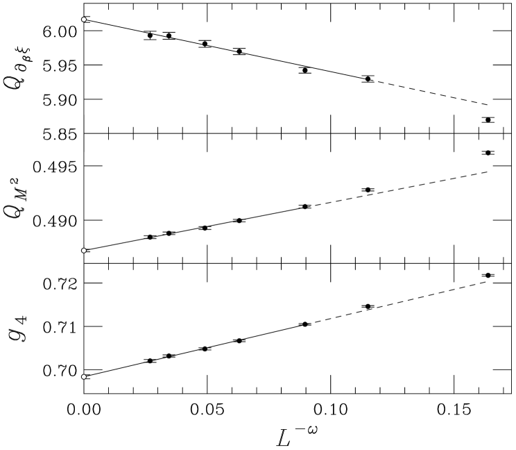
Figure 1: Infinite volume extrapolation for $Q_{\partial_{\beta}\xi}=2^{1+\frac{1}{\nu}}$, $Q_{M^{2}}=2^{-1-\eta}$, and $g_{4}$. The solid lines correspond to fits with $\omega=0.87$ from $L\geq L_{\mathrm{min}}$. A dashed line is plotted for $L<L_{\mathrm{min}}$.

In Fig. 1 we show graphically the fit quality for the quotients used to obtain the exponents as well as for $g_{4}$ cumulant.

We remark that the pair $(L,2L)$ having a systematic error in $\eta$ smaller than the final error in our extrapolation has $2L=2000$ ($2L=800$ for $\nu$). We recall that our largest pair has $2L=128$.

Values for the critical quantities obtained with MC by other authors are reported in table 4. For comparison, a recent series computation[26] yielded $\beta_{\mathrm{c}}=0.221659^{+2}_{-5}$. Only in Ref. [18] an infinite-volume extrapolation is considered for the critical exponents. A different approach has been used in Ref. [29], where the Hamiltonian is numerically tuned, in order to make the ${\mathcal{O}}(L^{-\omega})$ corrections for cumulant $g_{4}$ vanishing. This largely reduces the corrections-to-scaling for the exponents. However, the data of [29] have been analyzed as if these coefficients, $A_{O}$, would be exactly zero. However, there still is an error associated to the uncertainty in the assumption $A_{O}=0$, that has not been considered in Ref. [29]. In fact, there is nothing special in the value $A_{O}=0$, the only essential ingredient for the dramatic reducing of the error estimate is to neglect the error in $A_{O}$. Had we disregarded the error in $A_{Q_{O}}$, we would obtain $\nu=0.6294(2),\,\eta=0.0374(2)$. However, we do not believe this to be a valid procedure.

5 Site percolation results

The MC simulation in this case is rather different, since one generates directly independent configurations. We will work in the so-called canonical formulation in which the probability of finding a hole in a given lattice site is independent from the rest of sites.

It is very fast to generate the different configurations and most of computer time is employed in tracing the clusters. We generate 32 millions of samples for $L\leq 96$, 16 millions for $L=96,128$ and 4 millions for $L=192$. As we need individual measures for the $p$-extrapolation it is necessary to store them on disk as they are obtained from different processors. In all cases we simulate at $p=0.3116$ [5].

In table 5 we present the results for the exponents $\nu$ and $\eta$ as well as the $g_{2}$ and $g_{4}$ cumulants, obtained from different pairs of lattices.

$L$	$\nu$	$\eta$	$g_{2}$	$g_{4}$
8	0.8802(6)	-0.01531(12)	0.35395(11)	0.72353(9)
12	0.8847(6)	-0.03230(12)	0.35395(11)	0.72353(9)
16	0.8825(7)	-0.03844(12)	0.34854(10)	0.72074(10)
24	0.8807(10)	-0.04267(12)	0.34601(10)	0.71695(8)
32	0.8809(10)	-0.04423(10)	0.34559(10)	0.71499(9)
48	0.8771(14)	-0.04531(12)	0.34603(11)	0.71290(9)
64	0.8757(17)	-0.04539(10)	0.34638(10)	0.71195(8)
96	0.8796(33)	-0.04554(20)	0.34672(24)	0.71124(20)
$\infty$	0.8765(16)(2)	-0.04602(27)(7)	0.34675(26)(6)	0.71052(21)(19)

Table 5: Critical exponents for the site percolation obtained from pairs of type $(L,2L)$ obtained at $Q_{\xi}=2$. We also show the cumulants $g_{4}(L)$ and $g_{2}(L)$ at the same points. The last row correspond to an infinite volume extrapolation, showing the statistical error (first bar) and that coming from the uncertainty in $\omega$ (second bar).

$L$	$p_{\mathrm{c}}(\xi/L,L)$	$p_{\mathrm{c}}(g_{4},L)$
8	0.309761(7)	0.313201(11)
12	0.311034(5)	0.312454(7)
16	0.3113614(36)	0.3120770(49)
24	0.3115337(20)	0.3117950(26)
32	0.3115788(14)	0.3117007(19)
48	0.3115992(9)	0.3116390(12)
64	0.3116036(8)	0.3116214(12)
96	0.3116063(9)	0.3116122(11)

Table 6: Crossing points for $\xi/L$ and $g_{4}$ for the site percolation obtained from pairs of type $(L,2L)$.

Regarding $p_{\mathrm{c}}$, we show in table 6 the crossing points of $\xi/L$ and $g_{4}$ for pairs $(L,2L)$. We find a quite small, albeit significant, drift even in the largest lattices. Notice that the values for the $\xi/L$ ($g_{4}$) crossing are monotonically increasing (decreasing) with $L$. Thus, unless something weird happens with the scaling corrections, $p_{\mathrm{c}}$ is bounded from above and below and one can readily extract $p_{\mathrm{c}}=0.311609(3)$. However, a more precise $p_{\mathrm{c}}$ determination is possible using FSS techniques. We proceed as before to make a joint fit to Eq. (7) for all the data in table 6, excluding those for $L<L_{\mathrm{min}}$. The results are presented in table 7.

$L_{\mathrm{min}}$	$\chi^{2}/{\mathrm{d.o.f.}}$	$\omega$	$p_{\mathrm{c}}$
24	10.5/6	1.57(2)	0.3116092(5)(2)
32	0.65/4	1.62(4)	0.3116081(7)(2)
48	0.07/2	1.64(13)	0.3116075(11)(2)

Table 7: Infinite volume extrapolation of the crossing points for $g_{4}$ and $\xi/L$, including data from $L\geq L_{\mathrm{min}}$ in the site percolation, in order to obtain $\omega$ and $p_{\mathrm{c}}$.

The value of $\omega=1.62(13)$ is remarkably larger than in most of the 3D systems (slightly below 1), but agrees with the prediction of $\epsilon$-expansions, and lies between the $\omega_{\mathrm{2D}}=2$ of 2D site percolation [15] and the four dimensional value [10] $\omega_{\mathrm{4D}}=1.13(10)$. Moreover, our value for $\omega$ is in agreement with other MC determinations (see table 8).

Figure 2: $Q_{\partial_{\beta}\xi}=2^{1+\frac{1}{\nu}}$, $Q_{\chi}=2^{2-\eta}$, $g_{4}$ and $g_{2}$ for pairs ($L,2L$) as functions of $L^{-\omega}$. In the plot we use $\omega=1.62$.

In Fig. 2 we display the quotients of $\chi$ and ${\partial_{\beta}\xi}$, and the values of $g_{4}$ and $g_{2}$ as functions of $L^{-\omega}$ for $\omega=1.62$, measured at the points where $Q_{\xi}=2$. The linear behaviour is much less clear than in the Ising case. One should not be surprised by this fact since for such a large $\omega$ it is very unlikely a clear separation between the leading corrections-to-scaling (as $L^{-\omega}$) and the sub-leading ones. One should be specially worried with the analytical corrections that for most operators go as $L^{-\gamma/\nu}\approx L^{-2}$. A parameterization of the sub-leading corrections is far from the present MC capacities.

Fortunately, $\omega$ is large enough to make the extrapolation almost unnecessary. For $\nu$, we do not find significant deviations for $L\geq 48$ and one could be tempted of simply averaging, obtaining $\nu_{\mathrm{mean}}=0.8768(10)$. However, we find no reason to consider as vanishing the coefficient of $L^{-\omega}$, and this assumption underestimates the errors. We find a non zero value of $A_{Q_{O}}$ in the fits to Eq. (6) for $\eta$ and the cumulants. In the last raw of table 5 we present the results of these fits as well as the corresponding statistical errors, the second error bars corresponding to the uncertainty in $\omega$. This $\omega$-error allows to quantify the possible shift that could be expected if the dominant corrections-to-scaling were the analytical ones, as the behaviour is basically linear with $\omega$. One simply has to add 2.5 times the $\omega$ induced error to the central value for the extrapolation (the sign would be positive in the four cases). For $\nu$, $\eta$ and $g_{2}$, one can conclude that the systematic errors are hardly greater than the statistical one. For $g_{4}$ the former could be twice the latter. Our final results can be contrasted with other MC estimates in table 8.

Ref.	$p_{\mathrm{c}}$	$\sigma$	$\tau$	$\omega$
[13]	0.311604(6)		2.188(2)
[12]		0.445(10)	2.189(2)	1.61(5)
[14]	0.311600(5)		2.186(2)	1.77(13)
[8]				1.4
This work	0.3116081(7)(2)	0.4522(8)(1)	2.18906(6)(2)	1.62(13)

Table 8: Previous Monte Carlo determination of critical quantities for the 3D site percolation.

6 Conclusions

We have found that when measuring critical exponents and other universal quantities with high precision (below the 0.1%) with finite-size scaling techniques, a proper consideration of the corrections-to-scaling is mandatory.

We have studied two simple three dimensional models. The Ising model shows corrections that can be parameterized with the leading corrections-to-scaling term. It is possible to obtain a very safe infinite volume extrapolation that can be as far as 10 standard deviations from the largest lattice’s value.

In the site percolation, the behaviour is completely different. The leading corrections-to-scaling cannot be easily isolated from the higher order ones, since the first irrelevant exponent is very large. However, its largeness makes the results on the largest lattices very near the infinite volume limit, and the difficulties of the extrapolation are not overwhelming. We have also measured with high precision the values of two universal cumulants ($g_{4}$, $g_{2}$). The non-vanishing value of the latter shows that the susceptibility is not a self-averaging quantity.

References

- [1] L. P. Kadanoff, Physics 2, 263 (1966); K. Wilson, Phys. Rev. B4, 3174 (1971), ibid. B4, 3184 (1971), Phys. Rev. Lett. 28, 548 (1972).
- [2] J. Zinn-Justin, Quantum Field Theory and Critical Phenomena (Oxford Science Publications 1990).
- [3] R. Guida and J. Zinn-Justin, cond-mat/9803240.
- [4] M. N. Barber, Finite-size Scaling in Phase Transitions and Critical phenomena, edited by C. Domb and J.L. Lebowitz (Academic Press, New York, 1983) vol 8.
- [5] D. Stauffer and A. Aharony. Introduction to the percolation theory. (Taylor & Francis, London 1994)
- [6] P.W. Kasteleyn and C. M. Fortuin, J. Phys. Soc. Japan 26 (Suppl), 11 (1969).
- [7] M.N. Barber, R. B. Pearson, D. Toussaint and J. L. Richardson, Phys. Rev. B32, 1720 (1985).
- [8] J.M. Normand and H. J. Herrmann, Int. J. of Mod. Phys. C6, 813 (1995).
- [9] A. L. Talapov and H. W. Blöte, J. Phys. A29, 5727 (1996).
- [10] H.G. Ballesteros, L.A. Fernández, V. Martín-Mayor, A. Muñoz Sudupe, G. Parisi, J.J. Ruiz-Lorenzo, Phys. Lett. B400, 346 (1997);
- [11] G. Harris, Nucl. Phys. B418, 278 (1994).
- [12] C. D. Lorenz and R. M. Ziff, cond-mat/9710044. To be published in Phys. Rev. E.
- [13] P. Grassberger, J. Phys. A 25, 5867 (1992).
- [14] N. Jan and D. Stauffer, Int. J. Mod. Phys. C9, 341 (1998).
- [15] B. Nienhuis, J. Phys. A: Math. Gen. 15, 199 (1982).
- [16] H. G. Ballesteros, L.A. Fernández, V. Martín-Mayor, and A. Muñoz Sudupe, Phys. Lett. B378, 207 (1996); Phys. Lett. B387, 125 (1996); Nucl. Phys. B483, 707 (1997).
- [17] F. J. Wegner, Phys. Rev. B5, 4529 (1972).
- [18] H.W.J. Blöte, E. Luijten and J. R. Heringa, J. Phys. A28, 6289 (1995).
- [19] K. Binder, Z. Phys. B43, 119 (1981).
- [20] M. Falcioni, E. Marinari, M. L. Paciello, G. Parisi and B. Taglienti, Phys. Lett. D108, 331 (1982) ; A. M. Ferrenberg and R. H. Swendsen, Phys. Rev. Lett. 61, 2635 (1988).
- [21] F. Cooper, B. Freedman and D. Preston, Nucl. Phys. B 210, 210 (1989).
- [22] H.G. Ballesteros, L.A. Fernandez, V. Martí-Mayor, A. Muñoz Sudupe, G. Parisi, J.J. Ruiz-Lorenzo, Nucl. Phys. B512[FS], 681 (1998); J. Phys. A30, 8379 (1997); cond-mat/9802273, to be published in Phys. Rev. B.
- [23] U. Wolff, Phys. Rev. Lett. 62, 3834 (1989).
- [24] G. Parisi, F. Rapuano, Phys. Lett. B 157, 301 (1985).
- [25] M. Henkel, S. Andrieu, P. Bauer and M. Piecuch, cond-mat/9804201, to be published in Phys. Rev. Lett.
- [26] Z. Salman and J. Alder, Int. J. of Mod. Phys. C9, 195 (1998).
- [27] F. Livet, Europhys. Lett. 16, 139 (1991).
- [28] R. Gupta and P. Tamayo, Int. J. of Mod. Phys. C7, 305 (1996).
- [29] M. Hasenbusch, K. Pinn and S. Vinti, cond-mat/9804186.