Friedel Oscillations in the Open Hubbard Chain

Abstract

Using the Density Matrix Renormalization Group (DMRG), we calculate critical exponents for the one-dimensional Hubbard model with open boundary conditions with and without additional boundary potentials at both ends. A direct comparison with open boundary condition Bethe Ansatz calculations provides a good check for the DMRG calculations on large system sizes. On the other hand, the DMRG calculations provide an independent check of the predictions of Conformal Field Theory, which are needed to obtain the critical exponents from the Bethe Ansatz. From Bethe Ansatz we predict the behaviour of the $1/L$-corrected mean value of the Friedel oscillations (for the density and the magnetization) and the characteristic wave vectors, and show numerically that these conjectures are fulfilled with and without boundary potentials. The quality of the numerical results allows us to determine, for the first time, the behaviour of the coefficients of the Friedel oscillations as a function of the the Hubbard interaction.

I Introduction

Recent Bethe Ansatz studies of the one-dimensional Hubbard model with open boundaries subject to boundary chemical potentials or magnetic fields [1, 2, 3, 4] have opened new possibilities to apply the predictions of Boundary Conformal Field Theory [5, 6, 7] for the asymptotics of correlation functions to quantum impurity problems. As in the case of periodic systems, [8, 9, 10] the corresponding matrix elements cannot be computed directly but must be extracted from the scaling behaviour of the low–lying excited states. For generic filling and magnetization these finite size spectra allow the identification of the contributions from two massless bosonic sectors associated with the spin and charge excitations in a Tomonaga-Luttinger liquid.

A crucial step in these studies of systems with open boundary conditions is the correct interpretation of the finite-size spectra obtained from the Bethe Ansatz. These spectra determine both the bulk correlation functions, which are independent of the boundary fields, and the nonuniversal dependence of boundary phenomena such as the orthogonality exponent or X-ray edge singularities on the strength of the scatterer. Hence both in the requirement of conformal invariance and in the analysis of the finite-size spectra, the computation of correlation functions relies on assumptions which need to be verified by a more direct method, most notably by numerical calculations. Of course, comparison with exact results is also of interest for the numerical calculation: predictions of critical exponents for microscopic models allow the algorithms to be improved, which can then, in turn, be expected to produce better and more reliable results for more general systems.

These considerations motivate our study of the Friedel oscillations for the single particle density and magnetization in the open Hubbard chain with boundary chemical potentials, which is described by the Hamiltonian

$${\cal H}= - \sum_{\sigma,j=1}^{L-1}\left(c_{j,\sigma}^{\dagger}c_{j+1,\sigma}+{\rm h.c.}\right)+U\sum_{j=1}^{L}n_{j,\uparrow}n_{j,\downarrow}$$ (1)

$$- p\left(n_{1,\uparrow}+n_{1,\downarrow}+n_{L,\uparrow}+n_{L,\downarrow}\right),$$ (2)

where the lattice has $L$ sites, $c_{j,\sigma}^{\dagger}$ ($c_{j,\sigma}$) creates (destroys) an electron on site $j$, $n_{j,\sigma}=c_{j,\sigma}^{\dagger}c_{j,\sigma}$, and we have made the hopping integral dimensionless so that the Coulomb repulsion $U$ and the on–site potential $p$ are measured in dimensionless units.

Numerical calculations of critical exponents in low dimensional systems such as magnetic chains or electronic systems have a long history . Due to the need to consider systems of sufficient size, many earlier studies have used Quantum Monte Carlo methods to treat systems with periodic boundary conditions (PBC). [11] More recently, the Density Matrix Renormalization Group (DMRG) [12, 13] has become a new and powerful method especially suited to the study of one dimensional systems with open boundary conditions (OBC). [14, 15] However systems with PBC have also been studied with this method. [16, 17, 18]

In the usual approach to the calculation of correlation functions with DMRG one considers large systems and averages over an ensemble of correlation functions located sufficiently far from the boundaries. In the thermodynamic limit, this procedure removes the Friedel oscillations due to the boundary and gives the bulk behaviour of the quantity in question.

Here we want to make use of the existence of the exact solution of Eq. (2) in two ways in order to prepare the way for further extensions of the method: First, we use the quantities obtained from the Bethe Ansatz to provide checks of the numerical method at large system sizes. Second, we use the information contained in the oscillating behaviour to obtain more reliable results for the critical exponents.

This paper is organized as follows. In Sec. II, we give a short description of the Bethe Ansatz and DMRG methods, citing the relevant results from the Bethe Ansatz and Conformal Field Theory (CFT) concerning Friedel oscillations. In Sec. III, we study the Friedel oscillations of the density $N(x)$ and the magnetization $M(x)$. Combining the CFT results with those for noninteracting fermions, we obtain conjectures for the explicit form of the Friedel oscillations. After introducing the fit method used to obtain the exponents and coefficients from the DMRG results, we check the conjectures for two fixed densities and varying on–site interaction $U$. In addition, we study the dependence of the exponents and coefficients on the boundary potential $p$ at one density.

II Methods

A Bethe Ansatz

The one-dimensional Hubbard model with OBC, Eq. (2), can be solved using the coordinate Bethe ansatz. The symmetrized Bethe Ansatz equations (BAE) determining the spectrum of ${\cal H}$ in the $N_{e}=N_{\uparrow}+N_{\downarrow}$-particle sector read [1, 2, 3, 4]

$$e^{ik_{j}2L}B_{c}(k_{j})=\prod_{\beta=-N_{\downarrow}}^{N_{\downarrow}}\frac{\sin(k_{j})-\lambda_{\beta}+iu}{\sin(k_{j})-\lambda_{\beta}-iu}$$ (3)

(4)

$$B_{s}(\lambda_{\alpha})\prod_{j=-N_{e}}^{N_{e}}\frac{\lambda_{\alpha}-\sin(k_{j})+iu}{\lambda_{\alpha}-\sin(k_{j})-iu}=\prod_{\beta=-N_{\downarrow}\atop\beta\not=\alpha}^{N_{\downarrow}}\frac{\lambda_{\alpha}-\lambda_{\beta}+2iu}{\lambda_{\alpha}-\lambda_{\beta}-2iu}$$ (5)

$$j=-N_{e},\ldots,N_{e}\quad;\quad\alpha=-{N_{\downarrow}},\ldots,{N_{\downarrow}}$$ (6)

where we have defined $u=U/4$ and identified the solutions $k_{-j}=-k_{j}$ and $\lambda_{-\alpha}=-\lambda_{\alpha}$ in order to simplify the BAE. The boundary terms read

$$B_{c}(k) = \left(\frac{e^{ik}-p}{1-pe^{ik}}\right)^{2}\frac{\sin(k)+iu}{\sin(k)-iu}\,,$$ (7)

$$B_{s}(\lambda) = \frac{\lambda+2iu}{\lambda-2iu}\,.$$ (8)

Since the BAE are already symmetrized and the solutions $k=0$ and $\lambda=0$ have to be excluded, the energy of the corresponding eigenstate of Eq. (2) is given by

$$E=1-\sum_{j=-N_{e}}^{N_{e}}\cos{}(k_{j}).$$ (9)

In Refs. [2, 3, 4] the ground state and the low–lying excitations were studied for small boundary fields. In Ref. [19] the existence of boundary states in the ground state for $p>1$ was established. Bound states occur as additional complex solutions for the charge and spin rapidities.

Here we will use the explicit form of the BAE, Eq. (6), to check the energy convergence of the DMRG results for finite $L$. Furthermore, the expectation values of the density at the boundaries can be calculated from the derivative of the energy with respect to $p$ (cf. Sec. II B) allowing another check of the numerics. Finally, the value of the magnetization at the boundaries for vanishing $p$ can be calculated with a slightly modified Bethe–Ansatz (i.e. with a magnetic field at the boundary, see Refs. [3, 4]).

Using standard procedures, the BAE for the ground state and low–lying excitations can be rewritten as linear integral equations for the densities $\rho_{c}(k)$ and $\rho_{s}(\lambda)$ of real quasi-momenta $k_{j}$ and spin rapidities $\lambda_{\alpha}$, respectively:

$$\left(\begin{array}[]{c}\rho_{c}(k)\\[5.0pt] \rho_{s}(\lambda)\end{array}\right)=\left(\begin{array}[]{c}{1\over\pi}+{1\over L}\hat{\rho}_{c}^{0}(k)\\[5.0pt] {1\over L}\hat{\rho}_{s}^{0}(\lambda)\end{array}\right)+K*\left(\begin{array}[]{c}\rho_{c}(k^{\prime})\\[5.0pt] \rho_{s}(\lambda^{\prime})\end{array}\right)\$$ (10)

with the kernel $K$ given by

$$K=\left(\begin{array}[]{cc}0&\cos{}(k)\ a_{2u}(\sin(k)-\lambda^{\prime})\\[5.0pt] a_{2u}(\lambda-\sin(k^{\prime}))&-a_{4u}(\lambda-\lambda^{\prime})\end{array}\right).$$ (11)

Here we have introduced $a_{y}(x)={1\over 2\pi}\frac{y}{y^{2}/4+x^{2}}$, and $f*g$ denotes the convolution $\int_{-A}^{A}dyf(x-y)g(y)$ with boundaries $A=k_{0}$ in the charge and $A=\lambda_{0}$ in the spin sector. The values of $k_{0}$ and $\lambda_{0}$ are fixed by the conditions

$$\int_{-k_{0}}^{k_{0}}dk\rho_{c}=\frac{2\left[N_{e}-C_{c}\right]+1}{L}\quad$$ (12)

and

$$\int_{-\lambda_{0}}^{\lambda_{0}}d\lambda\rho_{s}=\frac{2\left[N_{\downarrow}-C_{s}\right]+1}{L},$$ (13)

where $C_{c}$ $(C_{s})$ denotes the number of complex $k$ $(\lambda)$–solutions present in the ground state.[19] In addition to the boundary terms in Eq. (8), the driving terms $\hat{\rho}_{c}^{0}$ and $\hat{\rho}_{s}^{0}$ depend on whether or not the complex solutions are occupied or not. The explicit form can be found in Refs. [2, 3, 4, 19]. The presence of these $1/L$ corrections leads to the shifts

$$\theta^{c}_{p}={1\over 2}\left(L\int_{-k_{0}}^{k_{0}}dk\hat{\rho}_{c}-1+2C_{c}\right)$$ (14)

$$\theta^{s}_{p}={1\over 2}\left(L\int_{-\lambda_{0}}^{\lambda_{0}}d\lambda\hat{\rho}_{s}-1+2C_{s}\right),$$ (15)

where $\hat{\rho}_{c}$ and $\hat{\rho}_{s}$ denote the solution of Eq. (10) without the $1/\pi$ driving term, i.e. the bulk system solution.

Here we will be mainly interested in the exponents of the Friedel oscillations, given in Table I. The quantity that determines the critical exponents is the dressed charge matrix ${\bf Z}$: [8, 20]

$${\bf Z}=\left(\begin{array}[]{cc}Z_{cc}&Z_{cs}\\ Z_{sc}&Z_{ss}\end{array}\right)=\left(\begin{array}[]{cc}\xi_{cc}(k_{0})&\xi_{sc}(k_{0})\\ \xi_{cs}(\lambda_{0})&\xi_{ss}(\lambda_{0})\end{array}\right)^{\top}$$ (16)

which is defined in terms of the integral equation

$$\left(\begin{array}[]{cc}\xi_{cc}(k)&\xi_{sc}(k)\\ \xi_{cs}(\lambda)&\xi_{ss}(\lambda)\end{array}\right)=\left(\begin{array}[]{cc}1&0\\ 0&1\end{array}\right)+K^{\top}*\left(\begin{array}[]{cc}\xi_{cc}(k^{\prime})&\xi_{sc}(k^{\prime})\\ \xi_{cs}(\lambda^{\prime})&\xi_{ss}(\lambda^{\prime})\end{array}\right)\,.\$$ (17)

In Ref. [21] it was shown that the $n$-point correlation functions of the open boundary system are related to the $2n$-point functions of the periodic boundary system. Thus the expectation value of the local density in the open system, $\langle N(x)\rangle_{o}$ can be extracted from the two–point correlation function $\langle N(z_{1})N(z_{2})\rangle_{p}$ of the periodic system (see also Ref. [22] where a spinless fermion model was considered). We can therefore use the results obtained in Refs. [8] and [9] for the density–density correlation function. As a function of $z_{c}=x+iv_{c}t$ and $z_{s}=x+iv_{s}t$ (where $v_{c}$ and $v_{s}$ denote the Fermi velocities of the charge and spin sector, respectively), the asymptotic form of $G_{nn}(x,t)=\langle N(x,t)N(0,0)\rangle$ is

$$G_{nn}(x,t)=n_{e}^{2}+\frac{B_{\downarrow}\cos(2k_{F,\downarrow}x+\delta_{\downarrow})}{|z_{c}|^{2\gamma_{\downarrow,c}}|z_{s}|^{2\gamma_{\downarrow,s}}}$$ (18)

$$+ \frac{B_{\uparrow}\cos(2k_{F,\uparrow}x+\delta_{\uparrow})}{|z_{c}|^{2\gamma_{\uparrow,c}}|z_{s}|^{2\gamma_{\uparrow,s}}}+\frac{B_{n}\cos(2(k_{F,\uparrow}+k_{F,\downarrow})x+\delta_{n})}{|z_{c}|^{2\gamma_{n,c}}|z_{s}|^{2\gamma_{n,s}}},$$ (19)

with $k_{F,\uparrow,\downarrow}=\pi n_{\uparrow,\downarrow}$. The exponents are displayed in Table I. Eq. (LABEL:ddper) shows the oscillating terms which are the most relevant ones asymptotically. For vanishing magnetization the momenta $k_{F,\downarrow}$ and $k_{F,\uparrow}$ coincide, and one has to consider logarithmic corrections in $x$ (see Ref. [23]) – this case will not be considered below.

Following Cardy [21] one has to replace $|z_{c}|^{2}\rightarrow x$ and $|z_{s}|^{2}\rightarrow x$ to obtain $\langle N(x)\rangle_{o}$ from Eq. (LABEL:ddper). The final result is

$$\langle N(x)\rangle=n_{e} + A_{\downarrow}\frac{\cos(2k_{F,\downarrow}x+\varphi_{\downarrow})}{x^{\gamma_{\downarrow,c}+\gamma_{\downarrow,s}}}+A_{\uparrow}\frac{\cos(2k_{F,\uparrow}x+\varphi_{\uparrow})}{x^{\gamma_{\uparrow,c}+\gamma_{\uparrow,s}}}$$ (21)

$$+ A_{n}\frac{\cos(2(k_{F,\uparrow}+k_{F,\downarrow})x+\varphi_{n})}{x^{\gamma_{n,c}+\gamma_{n,s}}}.$$ (22)

The correlation function $G_{\sigma\sigma}^{z}\sim\langle M(x,t)M(0,0)\rangle$ with magnetization $M=N_{\uparrow}-N_{\downarrow}$ has the same critical behaviour as $G_{nn}(x,t)$. Therefore $\langle M(x)\rangle$ has the same form as $\langle N(x)\rangle$, but with different coefficients $A_{\alpha}$.

B Density Matrix Renormalization Group

The density matrix renormalization group method (DMRG) [12, 13] has become one of the most powerful numerical methods for calculating the low-energy properties of one-dimensional strongly interacting quantum systems. The expectation values of equal-time operators in the ground state, such as the local density or magnetization which interest us here, can be calculated with very good accuracy on quite large systems (on lattices of up to $L=400$ sites in this paper). As we will see, access to such large system sizes is essential for the real space fitting method used to extract the coefficients and exponents of the Friedel oscillations (see Sec. III B). In the DMRG, open boundaries are also the most favourable type of boundary conditions numerically: for a given number of states kept (which corresponds to the amount of computer time needed) the accuracy in calculated quantitites such as the ground state energy is, in general, orders of magnitude better for open boundary conditions than for periodic boundary conditions. [13, 24]

In this work the finite system DMRG method is used: after the system is built up to a given size using a variation of the infinite system method, a number of finite-system iterations are performed in which the overall size of the system (i.e. the superblock) is kept fixed, but part of the system (the system block) is built up. Optimal convergence is attained by increasing the number of states kept on each iteration, and the convergence of the exact diagonalization step is improved by keeping track of the basis transformations and using them to construct a good initial guess for the wavevector.[25] For all calculations shown in this paper, we have performed 5 iterations with a maximum of $m=600$ states kept. The resulting discarded weight of the density matrix was ${\cal O}(10^{-7})$ and below.

We illustrate the convergence of the algorithm explicitly in Figs. 1–3. One finds that for all the parameters which are used in this paper the ground-state energy per site is accurate to ${\cal O}(10^{-6})$ or less, Fig. 1, while the expectation value of the density at the first site (or at the last site, due to symmetry) is accurate to ${\cal O}(10^{-5})$, as can be seen in Fig. 2.

TABLE I.: Exponents $\gamma_{\alpha,c}$ and $\gamma_{\alpha,s}$ as a function of the elements of the dressed charge matrix.

	$\gamma_{\alpha,c}$	$\gamma_{\alpha,s}$
$\alpha=\downarrow$	$(Z_{cc}-Z_{sc})^{2}$	$(Z_{cs}-Z_{ss})^{2}$
$\alpha=\uparrow$	$Z_{sc}^{2}$	$Z_{ss}^{2}$
$\alpha=n$	$Z_{cc}^{2}$	$Z_{cs}^{2}$

FIG. 1.: The difference between the ground state energy per site calculated with the DMRG, $E_{0}^{D}$, and the exact BA-energy, $E_{0}^{B}$, as a function of the number of DMRG iterations for a typical system ($L=400$, $n_{e}=0.55$, $n_{\uparrow}=0.35$, $U=10$ and $p=0$).

FIG. 2.: The difference between the expectation value of the density at site 1 calculated with DMRG, $N_{1}^{D}$, and with BA, $N_{1}^{B}$, for the fillings $n_{e}=0.55$ and $n_{e}=0.70$ without boundary fields.

The magnetization shows an analogous behaviour but with results correct up to ${\cal O}(10^{-4})$, Fig. 3. It is also interesting to note that for $U\leq 10$ there is no strong $U$-dependence of the accuracy of either the density or the magnetization expectation values.

We now want to examine the effect of switching on the boundary fields simultaneously at the first and last sites on the quality of the DMRG results. In order to do this, we compare the mean density $\langle N_{1}(p)\rangle$ from DMRG calculations with Bethe Ansatz results calculated in the thermodynamic limit. Within the Bethe Ansatz, the mean density is calculated from the derivative of $\langle{\cal H}\rangle$ with respect to the boundary field $p$.

FIG. 3.: The difference between the expectation value of the magnetization at site 1 calculated with DMRG, $M_{1}^{D}$, and with BA, $M_{1}^{B}$, for $n_{e}=0.55$ and $n_{e}=0.70$, without boundary fields.

FIG. 4.: The expectation value of $\langle N_{1}\rangle$ for different values of the interaction $U$ and boundary fields $p$ on a $L=100$ lattice with $n_{e}=0.55$ and $n_{\uparrow}=0.35$. The solid lines represent the exact solutions in the thermodynamic limit, while the symbols are DMRG results.

The numerical results, shown in Fig. 4 on an $L=100$ lattice for electron density $n_{e}=0.55$, $n_{\uparrow}=0.35$ and for two values of the interaction $U$, are again in very good agreement with the values for the thermodynamic limit. The difference $N_{1}^{\rm D}-N_{1}^{\rm B}$ is now ${\cal O}(10^{-3})$. While this seems to be worse than the $p=0$ case, we have neglected finite-size corrections to $\langle N_{1}\rangle$ since we have compared to thermodynamic limit Bethe Ansatz calculations. If we explicitly take the $1/L$ corrections to the Bethe Ansatz values into account, we find agreement to ${\cal O}(10^{-5})$. This value is already smaller than the $1/L^{2}$-corrections so that finally we state that $\langle N_{1}\rangle$ is accurate to ${\cal O}(10^{-4})$.

III Friedel Oscillations

In general, the presence of an impurity or boundary in a one-dimensional fermion system leads to Friedel oscillations in the density, which have the general form

$$\delta\rho(x)\sim{\cos(2k_{F}x+\varphi)\over x^{\gamma}}\ ,$$ (23)

where the exponent $\gamma$ depends on the interaction. In addition to numerical studies of these oscillations for spinless fermions [17] and Kondo–Systems [18], several theoretical attempts have been made to clarify the role of interaction. Using bosonization it is possible to obtain the asymptotic exponents as a function of the interaction parameters and corrections to the power–law behaviour of Eq. (23).[26, 27] CFT results were used to calculate the interaction dependence of the exponent $\gamma$ for interacting spinless fermions. [22] Here we start with noninteracting fermions to obtain some conjectures for the connection between the explicit form of the Friedel oscillations and Bethe Ansatz results. These conjectures will then be checked using the DMRG results.

A Noninteracting Fermions

By considering only spin-$\uparrow$ electrons without any boundary potential, one can easily obtain the expectation value of the electron density:

$$N(x)={N_{\uparrow}+{1\over 2}\over L+1}-{1\over 2(L+1)}\frac{\sin\left(2\pi x{N_{\uparrow}+1/2\over L+1}\right)}{\sin\left({\pi x\over L+1}\right)}.$$ (24)

In the limit $L\to\infty$ and $x\ll L$ the density is given by

$$N(x) = n_{\uparrow}-{n_{\uparrow}-{1\over 2}\over L}-{\sin\left(2\pi x(n_{\uparrow}-{n_{\uparrow}-{1\over 2}\over L})\right)\over 2\pi x}$$ (25)

$$= n_{\uparrow}-{\theta^{c}_{0}\over L}-{\sin\left(2\pi x(n_{\uparrow}-{\theta^{c}_{0}\over L})\right)\over 2\pi x},$$ (26)

with $\theta^{c}_{0}$ defined in Eq. (14). The density $N(x)$ can also be calculated explicitly when the boundary field $p=1$. It then has the same structure as Eq. (26).

If one assumes that the Friedel oscillations in the interacting system have an analogous structure to those in the non-interacting system, one can combine Eqs. (22) and (26) to obtain the following conjectures for the finite-size shifts of the average density, average magnetization and the characteristic wave vectors in the interacting system:

$$\overline{n}=n_{e}-{\theta_{n}\over L},\qquad\overline{m}=m-{\theta_{m}\over L}$$ (27)

$$k_{F,\downarrow}=\pi\left(n_{\downarrow}-{\theta_{\downarrow}\over L}\right),\qquad k_{F,\uparrow}=\pi\left(n_{\uparrow}-{\theta_{\uparrow}\over L}\right)$$ (28)

with $\theta_{\downarrow}=\theta^{s}_{p},\theta_{\uparrow}=\theta^{c}_{p}-\theta^{s}_{p},\theta_{n}=\theta^{c}_{p}$ and $\theta_{m}=\theta^{c}_{p}-2\theta^{s}_{p}$.

B Fit procedure

Previously, several methods have been used to obtain asymptotic exponents of correlation functions using numerical data.[11, 16, 28] All of these methods use the $L$–dependence of the fourier-transformed correlation functions near the relevant peaks $k_{\alpha}$ $(\alpha=\uparrow,\downarrow,n)$ in Fourier space to extract the exponents. Due to the fact that only systems with periodic boundary conditions were considered, the $k_{\alpha}$ were all independent of $L$. This $L$-independence seems to be crucial for these methods to work; we were not able to extract a reasonable exponent with any of these methods on a system with open boundary conditions.

Therefore, we fit the DMRG results for $N(x)$ and $M(x)$ to the real-space test function

$$f(x)=\left\{\begin{array}[]{c}\overline{n}\\ \overline{m}\end{array}\right\}+\sum_{\alpha\in\{\uparrow,\downarrow,n\}}{A_{\alpha}\sin(2k_{\alpha}x+\varphi_{\alpha})\over x^{\gamma_{\alpha}}}$$ (31)

$$+{A_{\alpha}\sin(2k_{\alpha}x+\varphi_{\alpha})\over(L+1-x)^{\gamma_{\alpha}}}$$ (32)

which explicitly includes the momenta as fit parameters. Here the second term is included due to symmetry. There are a total of 13 fit parameters in this function, a prohibitively large number to do a simultaneous fit of all parameters. However, if we only consider systems in which the three peaks in the Fourier–spectrum are well seperated, there is an effective fit of 4 parameters to every peak. As we will see, the peak at $k_{n}$ is supressed for small $U$, reducing the number of fit parameters to 9 for only two peaks. The amplitudes $A_{\alpha}$ will be assumed to be positive, with any sign given by the phase $\varphi_{\alpha}$. We fit to the magnetization $M(x)$ and the density $N(x)$ independently.

The right side of Eq. (26) is only valid for $x\ll L$. In addition, the CFT results are valid only asymptotically for large distances. As a consequence and compromise, we do not use the density information on the first five and last five lattice points.

We perform the least squares fit in two stages. In the first stage, the start parameters of the subsequent fit are determined using simulated annealing. The final fit is performed using a combined Gauss–Newton and modified Newton algorithm (using the NAG routine E04FCF). To estimate the fit error, 10 fits are performed for each system with 10% of the points randomly excluded from each fit.

C Results

Before discussing the results for the Friedel oscillations in detail, we make some general comments on the numerical results. As described in Sec. III B, we calculate the quantities for the density and magnetization oscillations by applying a 13-parameter fit. Fitting to this many parameters requires the use of large system sizes. While the numerical expense for the DMRG procedure grows linearly with the system size for a fixed number of states kept, the accuracy in the energy and in the local density and magnetization decreases with the system size, especially in the Luttinger liquid regime. [24] We have compared the accuracy of the DMRG results with the accuracy and convergence of the fitting procedure for different lattice sizes from $L=300$ to $L=500$ and have decided that $L=400$ yields optimal results for the amount of computing power available. However, results within this range of system sizes are in agreement to within DMRG and fitting errors.

Another important issue is the influence of the boundary potentials on the fitting method and on the Friedel oscillations (discussed in Sec. III C 3). As the boundary potential $p$ is increased, bound states will develop at site 1 and site $L$.[19] In order to avoid these bound states in the fitting procedure, one has to enlarge the range in which the local density $N(x)$ is disregarded from 5 (i.e. $x,L-x-1\leq 5$) at $p=0$ to about 20 at $p=9.9$.

The discussion of the next three sections will focus on comparing the BA/CFT predictions for the different fit parameters with the DMRG results, especially on checking the conjectures from Eqs. (27) and (28). We also compare the numerical results to the different exactly known values for different limits such as the limit of noninteracting fermions, $U\to 0$.

1 Density $n_{e}=0.55$

We first examine the Fourier transform of the local electron density $N(x)$, defined as

$$N(k,U)=\sum_{x=1}^{L}\cos\left(k(x-{1\over 2})\right)N(x,U)$$ (33)

with $k={2\pi j\over L}$ and $j=0,\ldots,{L\over 2}-1$. (Due to symmetry $N(k,U)$ vanishes for odd multiples of ${\pi\over L}$.) The quantity $N(k,U)$ is displayed in a three-dimensional plot in Fig. 5(a). Distinct peaks at the three wave vectors, $k_{\uparrow}$, $k_{\downarrow}$, and $k_{n}$ can clearly be seen. Note that we have chosen $n_{e}$ and $n_{\uparrow}$ so that these three peaks are well-separated. However, the peak at $k_{n}$ becomes very lightly weighted and therefore ill-defined for $U<1$. In fact, we have found that it is not possible to locate the third momentum $k_{n}$ for $U<1$ using the 13-parameter fit procedure described in Sec. III B. Therefore, we fit $N(x)$ using only 9 parameters for $U=0.1$ and $U=0.5$. We display the fourier-transformed magnetization $M(k,U)$, defined analogously, in Fig. 5(b). Here the $k_{n}$ peak is even more

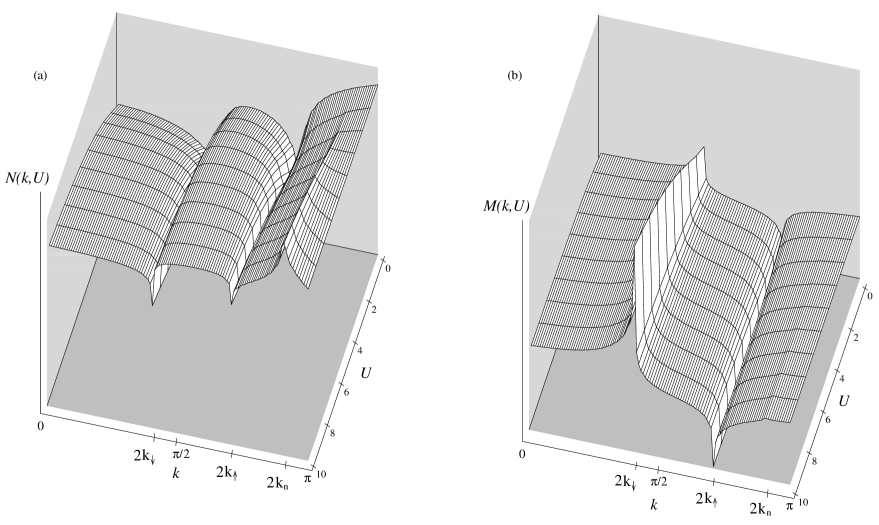
FIG. 5.: Fourier transformation of (a) the density $N(x)$ and (b) the magnetization $M(x)$ for several values of $U$ at the density $n_{e}=0.55$ and $n_{\uparrow}=0.35$. (The $k=0$ values are excluded.)

FIG. 6.: Difference $\theta_{\alpha}=(\alpha-\overline{\alpha})L$ for the density ($\alpha=n$) and the magnetization ($\alpha=m$) as a function of $U$ for $n_{e}=0.55$. The solid lines are the Bethe Ansatz conjectures $\theta_{\alpha}$.

poorly defined, and, in fact, is at best barely discernible, even at large $U$. Therefore, it is only possible to fit to two peaks using 9 parameters in the entire region from $U=0$ to $U=10$. For these fit procedures, we have found that the mean-squared deviation $\sigma^{2}=\sum_{x}(N(x)-f(x))^{2}$ is between ${\cal O}(10^{-7})$ and ${\cal O}(10^{-6})$ for the density and between ${\cal O}(10^{-6})$ and ${\cal O}(10^{-5})$ for the magnetization for all $U$ values. These limits will apply to all the fit results shown in this paper.

In Fig. 6 we show the $1/L$ corrections of the mean values $\overline{n}$ and $\overline{m}$ calculated with the DMRG and from Bethe Ansatz using the conjectures in Eq. (27). One can see that there is quite good agreement between the two calculations for all $U$.

The comparison of the exact asymptotic exponents at the different momenta with the numerical results is one of the most interesting and important features of this work because similar methods will then be able to be used to calculate properties not directly predictable with CFT/BA, and to treat systems that are not Bethe Ansatz solvable.

The exponents at $k_{\downarrow}$ and $k_{\uparrow}$, extracted from the density as well as from the magnetization data, are shown in Fig. 7. The difference between the fit–exponents and the CFT-prediction is less than 2% for the fits to the density and less than 3% for the fits to the magnetization. As mentioned above, we can obtain an exponent for the peak at $k_{n}$ from the density fit for $U\geq 1$ only, due to its small weight especially for small $U$. At $U=1$ the large error bars reflect a poor fit. Here we have only considered $U\leq 10$, for which $\gamma_{n}>\gamma_{\uparrow}$. A further increase in $U$ would lead to a region where $\gamma_{n}<\gamma_{\uparrow}$. A crossover between these two regions will be seen for the $n_{e}=0.70$ in the next section, for which it occurs at a somewhat lower $U$.

FIG. 7.: Exponents for the three peaks as a function of $U$ fitted for (a) the particle density and (b) the two peaks of the magnetization for $n_{e}=0.55$. The solid lines denote the CFT predictions from the Bethe Ansatz solution.

Due to the fact that we obtain only three independent exponents from the fitting procedures, it is not possible to determine all of the elements of the dressed charge matrix ${\bf Z}$. In fact, only the following combinations are relevant for the three exponents extracted: $Z_{cc}^{2}+Z_{cs}^{2},Z_{ss}^{2}+Z_{sc}^{2}$ and $Z_{cc}Z_{sc}+Z_{cs}Z_{ss}$. [28] It would be possible to uniquely determine all of the independent elements of the dressed charge matrix with additional information from, for example, any susceptibility [8] or from another correlation function with a different set of critical exponents. Relationships between the elements of the dressed charge matrix ${\bf Z}$ and the parameters of the Tomonaga–Luttinger model are given in Ref. [29].

Within the framework of CFT, the amplitudes $A_{\alpha}$ are completely undetermined. However, the form–factor approach [30] may lead to explicit results for the amplitudes in the future. For example, a conjecture of Lukyanov and Zamolodchikov [31] concerning the amplitude of the spin–spin correlation functions of the XXZ chain was recently confirmed by a fit to DMRG results. [14]

At this point, however, the fit results can only be compared to noninteracting fermions ($U=0$), for which $A_{\downarrow}=A_{\uparrow}={1\over 2\pi}$. As can be seen in Fig. 8, this value is in relatively good agreement (4% deviation) with the fit results. In addition, $A_{n}=0$ for $U=0$, in agreement

FIG. 8.: Amplitudes $A_{\alpha}$ fitted to (a) the density and (b) the magnetization as a function of $U$ for $n_{e}=0.55$. The solid lines are guides to the eye. The arrow denotes the value for the noninteracting fermions (=$1\over 2\pi$). Note that the amplitudes are, in general, different for the density and the magnetization.

with the $U=0$ extrapolated value in Fig. 8(a). The large error bars in $A_{n}$ at $U=1$ are due to the difficulty in fitting the $k_{n}$ peak for small $U$. Since the fitting procedure seems to work well for the exponents, and the amplitudes yield the correct $U=0$ limit, we feel that the calculation of the amplitudes is under good control. This is therefore the first determination of the qualitative as well as quantitive behaviour of these amplitudes.

The exact position of the momenta $k_{\uparrow}$ and $k_{\downarrow}$ are further fit parameters. The $1/L$ corrections to the thermodynamic value are plotted in Fig. 9. The fit values agree well with the Bethe Ansatz conjectures, except for the correction to $k_{\uparrow,m}$, which deviates from the Bethe Ansatz value for $U<4$. These deviations are probably due to problems with the fit. Note also that the Bethe Ansatz results for $\theta_{\alpha}$ are correct only up to ${\cal O}(1/L)$. The momentum $k_{n}$, which is not shown, is another independent fit parameter. The fit error in $k_{n}$ extracted from the fit to the density $N(x)$ is rather large for $U<4$. This is due to the fact that the peak at $k_{n}$ is not well–defined enough in this region to obtain the $1/L$ corrections to this momentum. Nevertheless the agreement between the fit values and the Bethe Ansatz conjectures is very good for

FIG. 9.: Difference $\theta_{\alpha,\beta}=(n_{\alpha}-{k_{\alpha,\beta}\over\pi})L$ for $\alpha=\downarrow,\uparrow$ as a function of $U$ for the density $n$ and magnetization $m$ for $n_{e}=0.55$. The solid lines denote the Bethe Ansatz conjectures $\theta_{\alpha}$ [see Eq. (28)].

$U>4$.

2 Density $n_{e}=0.70$

In this section, we examine the same quantities as in the previous section at a density of $n_{e}=0.70$. A treatment of this density is interesting for a number of reasons. Since we use the same numerical parameters for both densities, we can examine the density dependence of the error in truncating the Hilbert space using the DMRG. This density is also interesting because the BA/CFT calculations predict that the crossover between the $\gamma_{n}$ and $\gamma_{\uparrow}$ exponents will take place within the range of interaction treated here, $U=0\ldots 10$.

The Fourier transforms of the local density $N(x)$ and the magnetization $M(x)$ are shown in Fig. 10. Note that the momentum $k_{n}$ (wrapped back to the range $0$ to $\pi$) is now located between $k_{\downarrow}$ and $k_{\uparrow}$. As can be seen in Fig. 10(a), the peak in $N(x)$ at $k_{n}$ is not well-defined for $U<1$, so the $U=0.1$ and $U=0.5$ data are fitted using 9 parameters to fit two peaks. However, the $k_{n}$ peak in $M(x)$ is now more well-defined than for $n_{e}=0.55$, as can be seen in Fig. 10(b), and it is now possible to fit to all three momenta for $U\geq 2$. For smaller values of $U$ ($U=0.1$, $U=0.5$ and $U=1$), a nine-parameter fit is again made to two peaks.

The $1/L$ corrections to the mean values of the density and the magnetization, shown in Fig. 11, are in very good agreement with the BA conjectures, thereby providing a further confirmation of the predictions of Eqs. (27) and (28). The exponents extracted from the fit are shown in Fig. 12. The expected crossing of the two largest exponents at $U\approx 7$ can clearly be seen. For $\gamma_{\downarrow}$ and $\gamma_{\uparrow}$ obtained from the density fit, Fig. 12(a), the deviation from the CFT results is about 5% at most, with the largest errors occuring for $U>6$, especially in $\gamma_{\uparrow}$. As can be seen in Fig. 10(a), the peak at $k_{\uparrow}$ in $N(k,U)$ gets weaker for

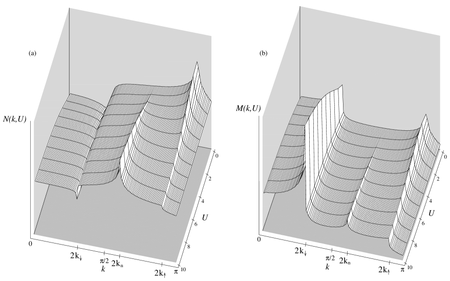
FIG. 10.: Fourier transformation of (a) the density $N(x)$ and (b) the magnetization $M(x)$ for several values of $U$ for the density $n_{e}=0.70$ with $n_{\uparrow}=0.55$ ($k=0$–values excluded). Note that the momentum $k_{n}$ is located between $k_{\downarrow}$ and $k_{\uparrow}$.

larger $U$, leading to a less effective fit. The agreement of the fitted exponents $\gamma_{n}$ with the CFT predictions is much better, with a deviation from the BA/CFT values of less than 1% for $U>1$. The exponents obtained from fits to the magnetization, Fig. 12(b), show deviations of up to about 6% from the BA/CFT results. For $U=9$ and $U=10$, the deviation is largest and the exponents coincidentally take on the same value. Again, this is probably due to larger errors in the fit because the peak at $k_{\uparrow}$ becomes weaker at larger $U$. One can see that the peaks at $k_{\uparrow}$ and $k_{n}$ are much less heavily weighted than the peak at $k_{\downarrow}$ at large $U$.

The amplitudes $A_{\downarrow}$ and $A_{\uparrow}$ extracted from the fit to the density, shown in Fig. 13(a), decrease monotonically with increasing $U$. The $U=0$ values agree with the exactly known value of $1/2\pi$ to within about 4%. The amplitude $A_{n}$, on the other hand, increases with increasing $U$. Its $U\rightarrow 0$ extrapolation agrees well with the value zero of the noninteracting fermions if the $U=1$ point, which cannot be very accurately determined, is excluded. The behaviour and even the quantitative values of all three coefficients are quite similar to the $n_{e}=0.55$ case shown previously in Fig. 8(a). The amplitudes obtained from the fit to the magnetization $M(x)$ are shown in Fig. 13(b). The amplitude $A_{\downarrow}$ behaves similarly to the $n_{e}=0.55$ case [Fig. 8(b)] in that it increases with increasing $U$, but $A_{\uparrow}$ shows different behaviour in that it reaches a maximum at $U\approx 1$ and then decreases. Both fit amplitudes yield the $U=0$ value of $1/2\pi$ to within 6%. The amplitude $A_{n}$ for the summed momenta, which could not be determined for $n_{e}=0.55$, increases monotonically with $U$, and its $U\rightarrow 0$ extrapolation agrees well with the value for noninteracting fermions, $A_{n}=0$.

The $1/L$ corrections to the momenta $k_{\downarrow}$ fitted for the density and the magnetization, shown in Fig. 14, are in good agreement with the Bethe Ansatz conjecture. The agreement is also fairly good for $\theta_{\uparrow,n}$, although the error of the fit is rather large for small $U$. However, the $\theta_{\uparrow,m}$ fit results do not match well with the conjecture. As we have seen in Fig. 10(b), the $k_{n}$ and $k_{\downarrow}$ peaks in $M(x)$ have much lower amplitudes than the $k_{\uparrow}$ peak, leading to lower accuracy in the fitting procedure. The fit results

FIG. 11.: Difference $\theta_{\alpha}=(\alpha-\overline{\alpha})L$ for density ($\alpha=n$) and magnetization ($\alpha=m$) as a function of $U$ for $n_{e}=0.7$. The solid lines are the Bethe Ansatz conjectures $\theta_{\alpha}$.

FIG. 12.: Exponents for the three peaks of (a) the particle density and (b) the magnetization as a function of $U$ for $n_{e}=0.7$. The solid lines denote the CFT predictions from the Bethe Ansatz solution.

for the exponents, Fig. 12(b) also had a rather large deviation from the CFT results in this regime. Thus it is not possible to confirm or deny the conjecture concerning the shift of $k_{\uparrow}$ for $M(x)$.

For $k_{n}$ the situation is even worse. Both density and magnetization fits lead to large fit errors for $U<4$. The deviation from the Bethe Ansatz conjectures is about $0.08$ in both fits, outside the range of the $1/L$ correction to $\theta_{n}$.

In summary, for $n_{e}=0.70$ the DMRG results for the mean density (magnetization, respectively) and the exponents are in good agreement with exact results from BA/CFT, further confirming Conformal Field Theory.

A detailed examination of the convergence of the DMRG shows that the numerical accuracy is actually slightly worse than the $n_{e}=0.55$ case, but this could be improved by increasing the number of states kept in the DMRG. We therefore expect to be able to apply these techniques reliably to obtain the boundary exponents and coeffients of other, non-Bethe-Ansatz solvable one-dimensional models.

FIG. 13.: Amplitudes $A_{\alpha}$ fitted to (a) the density and (b) the magnetization as a function of $U$ for $n_{e}=0.7$. The solid lines are a guide to the eye. The arrow denotes the value $1\over 2\pi$ of the noninteracting fermions. Note that the amplitudes are, in general, different for the density and the magnetization.

FIG. 14.: Difference $\theta_{\alpha,\beta}=(n_{\alpha}-{k_{\alpha,\beta}\over\pi})L$ for $\alpha=\downarrow,\uparrow$ as a function of $U$ for the density $n$ and magnetization $m$ for $n_{e}=0.7$. The solid lines denote the Bethe Ansatz conjectures $\theta_{\alpha}$ [see Eq. (28)].

3 Effect of boundary potentials

We now examine the effect of the boundary potential $p$ on the Bethe Ansatz predictions. We set $n_{e}=0.55$, $n_{\uparrow}=0.35$, and $U=8$ and consider six $p$ values, for which four qualitatively different Bethe Ansatz solutions exist. For $p=-0.5,\,0,\,0.5$, no bound state is present in the Bethe Ansatz ground state; we examine both repulsive and attractive fields. The values $p=2.6$ and $p=6$ are in a region in which the Bethe Ansatz has two complex $k$ solutions, one for each boundary potential at site $x=1$ and $x=L$. The $p=6$ ground state configuration contains, in addition, two complex $\lambda$ solutions. Finally, for $p=9.9$ there are four complex $k$ and two complex $\lambda$ solutions, corresponding to a bound pair of electrons at each end of the chain. Details of the structure of the ground state as a function of $p$ are given in Ref. [19].

The $p$-dependence of $N(k,p)$ and $M(k,p)$ at $U=8$ is not as strong as the $U$-dependence of $N(k,U)$ and $M(k,U)$ found previously. Since we have chosen a fairly large $U$, the peaks in the density $N(x)$ have enough weight to fit all three momenta. As was the case for $p=0$, the peak at $k_{n}$ in the magnetization is not pronounced enough to be fitted at any $p$.

The $1/L$ corrections to the mean values of the density and magnetization, Fig. 15, are again in very good agreement with the Bethe Ansatz conjectures, showing that Eqs. (27) and (28) are valid even in the different physical regions described above. Within the BA/CFT calculations, the values of the exponents are independent of the boundary potentials $p$. This agrees with the DMRG results, which we do not show here: the range of the exponents varies by at most 2% from the exact values for $p=0$ (after a larger number of lattice points are discarded from the fits in order to avoid the bound states at the ends).

The amplitudes also have no significant $p$-dependence. The density fit yields $A_{\downarrow}\approx A_{\uparrow}\approx 0.045$ and $A_{n}\approx 0.12$,

FIG. 15.: Difference $\theta_{\alpha}=(\alpha-\overline{\alpha})L$ for density ($\alpha=n$) and magnetization ($\alpha=m$) as a function of $p$ for $U=8$, $n_{e}=0.55$ and $n_{\uparrow}=0.35$. The solid lines are the Bethe Ansatz conjectures for $\theta_{\alpha}$.

FIG. 16.: Difference $\theta_{\alpha,\beta}=(n_{\alpha}-{k_{\alpha,\beta}\over\pi})L$ for $\alpha=\downarrow,\uparrow,n$ as a function of $p$ for the density $n$ and magnetization $m$ for $U=8$, $n_{e}=0.55$ and $n_{\uparrow}=0.35$. The solid lines denote the Bethe Ansatz conjectures $\theta_{\alpha}$ [see Eq. (28)].

while the magnetization fit yields $A_{\downarrow}\approx 0.28$ and $A_{\uparrow}\approx 0.21$. The absence of $p$-dependence at $U=8$ suggests that the interaction dependence of the coefficients should be that of Fig. 8, independent of the boundary fields $p$.

The effect of the boundary potential $p$ on the shift of the positions of the peaks is much larger than the effect of varying $U$ (compare Fig. 16 with Fig. 9). Since the fit results for all three $k$ values agree very well with the Bethe Ansatz conjectures, the confirmation of Eq. (28) is even more compelling than it was for the $U$–dependence.

IV Summary and Conclusions

We have carried out a detailed comparison between the exact Bethe Ansatz solution and Density Matrix Renormalization Group calculations for the one-dimensional Hubbard model with open boundary conditions both with and without an additional chemical potential at both ends. A direct comparison of the ground state energies as well as the density and magnetization at the ends of the chain has allowed us to estimate the accuracy of the DMRG on the large system sizes used in this work.

We have then compared the behaviour of the Friedel oscillations in the local density and local magnetization calculated directly using the DMRG with Conformal Field Theory predictions for the asymptotic forms for which the exponents can be calculated using the Bethe Ansatz. We have performed this check for two different fillings, $n_{e}=0.55$ and $n_{e}=0.70$ for the case without boundary potentials, $p=0$. We have obtained results consistent with the CFT predictions in all cases except those in which it is clear that the accuracy of the fitting procedure breaks down. Such a breakdown occurs when a particular peak in the fourier transform of the density or magnetization becomes lightly weighted and thus poorly defined. This occurs principally for the $k_{n}=(k_{F,\uparrow}+k_{F,\downarrow})$ peak, especially at small $U$ values. The good agreement between the CFT forms and BA values of the exponents and the DMRG calculations provides both a confirmation of the CFT predictions and a way to test the accuracy of the DMRG and of the effectiveness of fitting procedures for the Friedel oscillations.

In addition, we have proposed a relation between the $1/L$ corrected mean values in the density and magnetization and the $1/L$ corrections occuring in the BAE. This conjecture is supported by good agreement between mean values obtained from the fit to the DMRG data and the BAE results.

We have been able to extract for the first time the interaction dependence of the amplitudes for the Friedel oscillations, a property not possible to calculate in the framework of the CFT, and have found the correct behaviour in the $U\to 0$ limit.

Finally, we have turned on boundary chemical potentials at $n_{e}=0.55$ and examined the $p$-dependence of the critical exponents, the amplitudes and our conjectures for the behaviour of the mean density and magnetization. The different $p$-regimes that we have considered yield qualitatively distinct Bethe Ansatz solutions that are physically connected with the formation of different types of bound states at the system boundaries. In agreement with BA/CFT predictions, we have found that the critical exponents are independent of $p$ and that the influence of $p$ on the amplitudes is very weak. We have also found that our conjectures for the $1/L$ corrected mean values of the density, magnetization and the wave-vector hold in all of the physically different $p$-regimes.

The combination of analytical and numerical methods presented here has yielded new insights into both. The success of the numerical techniques will now allow the examination of more complicated systems that are not exactly solvable. Through comparison with the DMRG calculations, we have also been able to show that more information is contained in the BAE than is obtained from a direct interpretation via Conformal Field Theory.

- [1] H. Schulz, J. Phys. C 18, 581 (1985).
- [2] H. Asakawa and M. Suzuki, J. Phys. A 29, 225 (1996).
- [3] T. Deguchi and R. Yue, cond-mat/9704138 (unpublished).
- [4] M. Shiroishi and M. Wadati, J. Phys. Soc. Japan 66, 1 (1997).
- [5] J. L. Cardy, Nucl. Phys. B 324, 581 (1989).
- [6] I. Affleck and A. W. W. Ludwig, J. Phys. A 27, 5375 (1994).
- [7] I. Affleck, in Correlation effects in low-dimensional electron systems, Vol. 118 of Springer Series in Solid-State Sciences, edited by A. Okiji and N. Kawakami (Springer Verlag, Berlin, 1994), pp. 82–95.
- [8] H. Frahm and V. E. Korepin, Phys. Rev. B 42, 10553 (1990).
- [9] H. Frahm and V. E. Korepin, Phys. Rev. B 43, 5653 (1991).
- [10] N. Kawakami and S.-K. Yang, J. Phys. Condens. Matter 3, 5983 (1991).
- [11] S. Sorella, A. Parola, M. Parrinello, and E. Tosatti, Europhys. Lett. 12, 721 (1990).
- [12] S. R. White, Phys. Rev. Lett. 69, 2863 (1992).
- [13] S. R. White, Phys. Rev. B 48, 10345 (1993).
- [14] T. Hikihara and A. Furusaki, cond-mat/9803159 (unpublished).
- [15] V. Meden, P. Schmitteckert, and N. Shannon, Phys. Rev. B 57, 8878 (1998).
- [16] S. Qin, S. Liang, and Z. Su, Phys. Rev. B 52, R5475 (1995).
- [17] P. Schmitteckert and U. Eckern, Phys. Rev. B 53, 15397 (1996).
- [18] N. Shibata, K. Ueda, T. Nishino, and C. Ishii, Phys. Rev. B 54, 13495 (1996).
- [19] G. Bedürftig and H. Frahm, J. Phys. A 30, 4139 (1997).
- [20] F. Woynarovich, J. Phys. A 22, 4243 (1989).
- [21] J. L. Cardy, Nucl. Phys. B 240, 514 (1984).
- [22] Y. Wang, J. Voit, and F.-C. Pu, Phys. Rev. B 54, 8491 (1996).
- [23] T. Giamarchi and H. J. Schulz, Phys. Rev. B 39, 4620 (1989).
- [24] S. Kneer, Diploma Thesis, Universität Würzburg (unpublished).
- [25] S. R. White, Phys. Rev. Lett. 77, 3633 (1996).
- [26] M. Fabrizio and A. O. Gogolin, Phys. Rev. B 51, 17827 (1995).
- [27] R. Egger and H. Grabert, Phys. Rev. Lett. 19, 3505 (1995).
- [28] M. Ogata, T. Sugiyama, and H. Shiba, Phys. Rev. B 43, 8401 (1991).
- [29] K. Penc and J. Sólyom, Phys. Rev. B 47, 6273 (1993).
- [30] F. Lesage and H. Saleur, J. Phys. A 30, L457 (1997).
- [31] S. Lukyanov and A. Zamolodchikov, Nucl. Phys. B 493, 571 (1997).