[

Superflow-Stabilized Nonlinear NMR in Rotating ³He-B

Abstract

Nonlinear spin precession has been observed in ³He-B in large counterflow of the normal and superfluid fractions. The new precessing state is stabilized at high rf excitation level and displays frequency-locked precession over a large range of frequency shifts, with the magnetization at its equilibrium value. Comparison to analytical and numerical calculation indicates that in this state the orbital angular momentum $\vec{L}$ of the Cooper pairs is oriented transverse to the external magnetic field in a “non-Leggett” configuration with broken spin-orbit coupling. The resonance shift depends on the tipping angle $\theta$ of the magnetization as $\omega-\omega_{L}=(\Omega_{B}^{2}/2\omega_{L})(\cos\theta-1/5)$. The phase diagram of the precessing modes with arbitrary orientation of $\vec{L}$ is constructed.

]

The study of nonlinear NMR response in superfluid ³He started with the discovery of the Brinkman–Smith (BS) mode in ³He-A [2] and ³He-B [3] phases. These became the classic examples of nonlinear spin resonance in magnetically ordered superfluids. Their observation by Osheroff and Corruccini [4] opened the road to the discovery of new resonance states in ³He-B, such as space-coherent precession within a Homogeneously Precessing Domain (HPD) [5] or the newly found stable modes where the magnitude of the precessing magnetization differs from its equilibrium value [6]. An example of the latter is the family of half-magnetization modes (HM), where the precessing magnetization equals one half of the equilibrium value [7]. All of these are stable dynamic order parameter states and nonlinear solutions of the Leggett–Takagi spin dynamic equations. In principle, such states are similar to Q-balls, the coherent soliton-like nontopological states of relativistic quantum field theories, whose frequency and stability are determined by the conservation of the global charge, say, the baryonic charge [8]. In ³He-B spin dynamics the role of the global charge is played by the projection of the spin $S_{z}$ in the direction of the magnetic field $\vec{H}$, which determines, in part, the NMR frequency shift.

In these resonance modes the distinguishing factor is the orientation of the orbital angular momentum $\vec{L}$ of the Cooper pairs. In the BS and HPD modes, $\vec{L}$ is oriented along the applied magnetic field $\vec{H}$ via the spin-orbit (dipole) coupling, i.e. $\vec{L}\parallel\vec{H}$. In contrast, the HM modes form with $\vec{L}$ oriented spontaneously perpendicular to $\vec{H}$. So far, in the nonlinear regime the orientation of $\vec{L}$ has not been controlled by external means. Here we use vortex-free counterflow of the normal and superfluid components in a rotating container, to orient $\vec{L}$ along the flow direction. At high rotation velocity $\Omega$, the orienting effect on $\vec{L}$ from the flow far exceeds that from the dipole coupling. If the external magnetic field is oriented along the rotation axis ($\vec{H}\parallel\vec{\Omega}$), one can then study the unusual situation, when $\vec{L}\perp\vec{H}$. By measuring the tipping angle of the precessing magnetization $\vec{M}$ as a function of the applied frequency shift, we identify a new nonlinear resonance mode which greatly differs from the classic case of $\vec{L}\parallel\vec{H}$. In the linear regime the condition $\vec{L}\perp\vec{H}$ has been realized in earlier measurements in the parallel-plate geometry or in the presence of counterflow [9].

Experiment.—Our cw NMR setup in the rotating nuclear demagnetization cryostat has been described in Refs. [6, 10]. The ³He NMR sample is contained in a quartz glass cylinder with a radius $R=2.5$ mm. The measurements are performed at fixed frequency $\omega_{\rm rf}/2\pi=688$ kHz, using a linear field sweep centered around a Larmor field value of $H=21.2$ mT, with a homogeneity $\Delta H/H=2\cdot 10^{-4}$ over the sample volume. The signal is read with a lock-in amplifier, such that the component in phase with the excitation field $H_{\rm rf}$ is called dispersion $(\propto M_{x}=M_{\perp}\cos{\phi})$ and the out-of-phase component absorption $(\propto M_{y}=M_{\perp}\sin{\phi})$. The measuring range comprises counterflow velocities $\Omega R\leq 6.5$ mm/s, rf fields up to 0.03 Oe, temperatures (0.7—1) T_c, and pressures 0—12 bar.

At low excitation amplitude ($H_{\rm rf}\sim 0.003\,$Oe), when the tipping angle is a few degrees, the NMR response of ³He-B exhibits linear behaviour: The line shapes of the absorption and dispersion signals are independent of sweep direction, and the signal amplitudes increase linearly with excitation level. In vortex-free counterflow at sufficiently high velocity ($\Omega\gtrsim 0.5$ rad/s) the NMR absorption maximum is shifted from the Larmor value [9], as shown by the NMR spectrum in the inset of Fig. 1.

At high excitation levels the absorption and dispersion signal amplitudes increase faster than the rf field, and become highly asymmetric (Fig. 1). The nonlinear behavior becomes most pronounced while scanning the field in the upward direction towards the Larmor value until finally an abrupt jump appears from the precession at large tipping angle $\theta$ to the linear NMR regime with small $\theta$. If the excitation amplitude is increased, the jump usually moves to higher field. The field sweep in the opposite direction has significantly different shape and the regime of large tipping angles is not entered. The magnitude of the counterflow plays a crucial role (Fig. 2): With decreasing $\Omega$ both the maximum tipping angle and the range of frequency shifts quickly decrease. This means that the new state appears only at high counterflow velocities above the textural transition in which $\vec{L}$ is deflected into the plane transverse to $\vec{\Omega}$ in a significant part of the cross section of the sample cylinder [11].

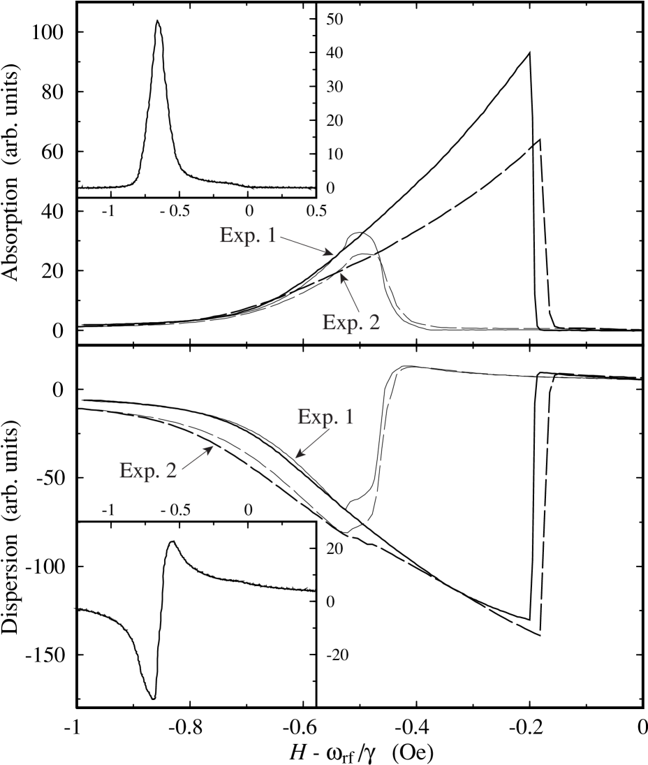
FIG. 1.: NMR response while the applied magnetic field $H$ is swept at constant rate $\dot{H}$ during continuous rf irradiation at fixed frequency $\omega_{\rm rf}$ ($\Omega=2.5$ rad/s, $P=0\,$bar, and $T\approx 0.88\,T_{c}$). Up sweeps are marked with thicker lines and down sweeps with thinner lines. Solid lines correspond to $H_{\rm rf}=0.02\,$Oe and $\dot{H}=0.017\,$Oe/s (Exp. 1), dashed lines to $H_{\rm rf}=0.027\,$Oe and $\dot{H}=0.034\,$Oe/s (Exp. 2). Note that at higher excitation lower absorption is measured for compensating the relaxation. (Insets) Line shapes of the signal in the linear regime at low exitation level ($\Omega=1.3$ rad/s, $P=2.0$ bar, $T=0.90\;T_{c}$, and $H_{\rm rf}=0.003$ Oe).

FIG. 2.: Transverse magnetization component $M_{\perp}$ as a function of field $H$, at different counterflow velocities in vortex-free rotation (listed in terms of $\Omega$ and the dimensionless variable $u$, calculated at the outer perimeter of the sample cylinder from Eq. (2)). Only upward sweeps of the field $H$ are shown, down sweeps depend less on $\Omega$ and are similar to those in Fig. 1. The temperature increases slowly during the measurement from $0.88\,T_{c}$ at the highest velocity to $0.92\,T_{c}$ at the lowest velocity. The normal state magnetization $\chi_{\rm N}H$ corresponds approximately to 200 units on the vertical scale ($P=0\,$bar, $H_{\rm rf}=0.027\,$Oe, and $\dot{H}=0.017\,$Oe/s).

We interprete these observations in the following manner. For fixed orientations of $\vec{S}$ and $\vec{L}$, the resonance frequency shift is determined by the dipole interaction. During the field sweep these vectors deflect from there equilibrium positions and the frequency of the resonance absorption changes. If the sweep is performed in a suitable direction, it may become possible to create a state where the resonance frequency stays locked to the external excitation frequency. In this case the increasing deflection of $\vec{S}$ causes the transverse magnetization $M_{\perp}$ to increase, which is observed in the experiment during a sweep towards the Larmor value as an increase in the dispersion and absorption signals. The tipping angle increases continuously with the field sweep as long as the rf pumping is sufficient to compensate for relaxation, which increases as the deviation of $\vec{S}$ from its equilibrium orientation increases. Finally the mode collapses, in a first order transition between two different dynamic order parameter states. This behaviour resembles that of an anharmonic oscillator in forced oscillation. The remarkable feature of ³He-B is that the rigidity from the order parameter coherence makes the superfluid to behave like a single oscillator.

Classification of modes.—An analytic description of spin precession with arbitrary orientations of $\vec{S}$ and $\vec{L}$ can be constructed, if we neglect magnetic relaxation and the interaction with the excitation field. The orientation of the orbital momentum, below denoted by the unit vector $\hat{l}=-\vec{L}/|\vec{L}|$, is fixed by the balance between its interactions with the counterflow and with the precessing spins via the dipole coupling. The former is written as

$$F_{\rm cf}=-{1\over 2}\rho_{a}((\vec{v}_{s}-\vec{v}_{n})\cdot\hat{l})^{2}~{}~{}.$$ (1)

Here $\rho_{a}=\rho_{s\perp}-\rho_{s\parallel}$ is the superfluid density anisotropy, caused by the magnetic field [12]. The relative magnitude of the counterflow and dipole energies is conveniently expressed in terms of a dimensionless velocity:

$$u={{15\rho_{a}\gamma^{2}(\vec{v}_{s}-\vec{v}_{n})^{2}}\over{4\chi\Omega_{B}^{2}}}\;,$$ (2)

where $\Omega_{B}(T,P)$ is the characteristic ³He-B frequency and a measure of the dipole energy. Spin precession is simplified in the high-field limit, when the dipole term is small compared to Zeeman energy, $-\vec{S}\cdot\gamma\vec{H}$, and can be considered as a perturbation. In zero order perturbation theory one has precession with the Larmor frequency, $\omega_{L}=\gamma H$. A first order correction gives the frequency shift from the precessing frequency $\omega$: $\omega-\omega_{L}=-\partial F_{D}/\partial S_{z}$, where $F_{D}$ is the dipole energy, averaged over the period of the precession. Here we consider only the case when the precessing spin has its equilibrium magnitude $S=\chi_{\rm B}H/\gamma$. For arbitrary orientation of the orbital momentum, the time-averaged dipole energy $F_{D}$ can be written as [13]

$$F_{D}=\frac{2}{15}\frac{\chi}{\gamma^{2}}\Omega_{B}^{2}[(s_{z}l_{z}-{1\over 2}+{1\over 2}\cos\Phi(1+s_{z})(1+l_{z}))^{2}+$$ (3)

$${1\over 8}(1-s_{z})^{2}(1-l_{z})^{2}+(1-s_{z}^{2})(1-l_{z}^{2})(1+\cos\Phi)]~{}.$$ (4)

The notations are: $s_{z}=S_{z}/|{\vec{S}}|=\cos{\theta}$, $l_{z}$ is the projection of the orbital momentum $\hat{l}$ on the direction of the magnetic field $\vec{H}$, and the angle $\Phi$ is a soft variable related to the ³He-B order parameter. The energy $F_{D}$ is also to be stationary with respect to $\Phi$: $\partial F_{D}/\partial\Phi=0$.

Thus by varying the dipole energy with respect to the spin $S_{z}$ (the analogue of the global charge) one obtains the precessing modes as a function of the frequency shift and of the other global charge $L_{z}$, which is kept fixed because of orbital viscosity. Omitting the limiting cases $\theta=0$ and $\theta=\pi$, we get three modes of precession

$$1) \cos\Phi=-{(1-2l_{z})(1-2s_{z})\over(1+s_{z})(1+l_{z})},$$ (6)

$$\hskip 60.00009pts_{z}={3-18l_{z}+15l_{z}^{2}+4w\over 15(1-l_{z})^{2}},$$

$$2) \cos\Phi=1,~{}~{}~{}~{}s_{z}=-{-1+4l_{z}+5l_{z}^{2}+4w\over-13+10l_{z}+35l_{z}^{2}},$$ (7)

$$3) \cos\Phi=-1,~{}~{}s_{z}=-\frac{3(1-l_{z}^{2})+4w}{3(1-l_{z})^{2}}.$$ (8)

Here $w$ is the dimensionless frequency shift:

$$w={{15\omega_{L}(\omega-\omega_{L})}\over{2\Omega_{B}^{2}}}\;.$$ (9)

In Fig. 3 the $l_{z}$—$s_{z}$ phase diagram is shown with the stable regions for each of the three modes. In the absence of counterflow, $u=0$, the dipole coupling orients the orbital momentum $\hat{l}$ along the magnetic field $\vec{H}$ in modes 1 and 2 and opposite to the field in mode 3. Then mode 1 becomes the BS state with zero frequency shift in the range $-{1\over 4}<s_{z}<1$ and $l_{z}=1$. Mode 2 reduces to the HPD state with $-1<s_{z}<-{1\over 4}$, $l_{z}=1$, and a frequency shift vs tipping angle dependence as $w=-2-8s_{z}$, while mode 3 transforms to the so-called HPD(2) which has not been seen experimentally [14]. In the generalized phase diagram of Fig. 3 with nonzero $u$, we retain these names for the regions in which their respective $u=0$ modes lie. In large counterflow linear NMR at small $\theta$ and nonlinear NMR at large $\theta$ are located in Fig. 3 on the $l_{z}=0$ axis and belong to the same class of BS states. During an up sweep the precession moves continuously from small to large $\theta$, until ultimately magnetic relaxation causes an instability and a first order transition takes $\theta$ back into the linear regime. This is similar to a gas-liquid transition, where no symmetry break occurs.

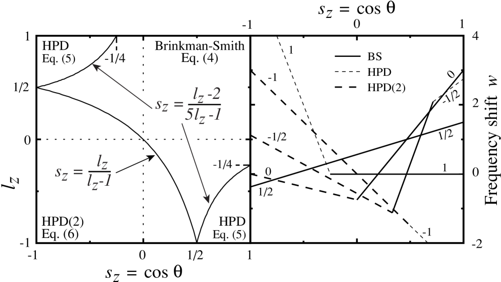
FIG. 3.: (Left) Phase diagram of the precessing states for arbitrary orientations of $\vec{L}$ and $\vec{S}$. (Right) Dependence of the frequency shift $w$ on the tipping angle $\theta$ for a few fixed values of $\hat{l}_{z}$ (marked for each line at its end point).

Limit of large counterflow.—In rapid rotation $u$ becomes large ($u\sim 15$) and the orbital momentum is rigidly forced into the transverse plane over most of the cross section of the sample cylinder: $l_{z}=0$. The HPD state does not exist in this limit, while the BS and HPD(2) modes have the frequency shifts

$$\displaystyle\omega-\omega_{L}={\Omega_{B}^{2}\over 2\omega_{L}}\left(\cos\theta-{1\over 5}\right)~{},~{}~{}~{}~{}~{}s_{z}>0~{}.$$ (10)

$$\displaystyle\omega-\omega_{L}=-{\Omega_{B}^{2}\over 10\omega_{L}}\left(1+\cos\theta\right)~{},~{}s_{z}<0~{}.$$ (11)

In Eq. (10) the linear regime of small $\theta$ corresponds to $s_{z}\approx 1$ and $w=3$ or $\omega-\omega_{L}=(2/5)\Omega_{B}^{2}/\omega_{L}$. In the nonlinear regime at large $\theta$ the frequency shift has a positive slope as a function of the longitudinal magnetization: $d\omega/d\cos\theta>0$. This suggests that in free precession in a pulsed NMR measurement homogeneous precession should become unstable and break into domains. In contrast, in continuous rf excitation the phase of the precession is locked to that of $H_{\rm rf}$ and no instability occurs. The HPD(2) shift in Eq. (11) has a negative slope, $d\omega/d\cos\theta<0$, and, since the conventional HPD state is unstable in counterflow, HPD(2) is thus the only inherently stable mode in large counterflow, with spontaneous phase-coherence in free precession. However, the HPD(2) mode displays large Leggett–Takagi relaxation because of its large deviation from the Leggett configuration. Presumably in the $T\rightarrow 0$ limit, where relaxation vanishes, the HPD(2) mode might become observable.

Comparison with experiment.—In Fig. 4 we plot the tipping angle $\theta$ from Eq. (10) as a function of the frequency shift $w$, along with the two measured NMR responses from Fig. 1. The frequency shift, at which the new mode collapses in the experiment, is determined by the relaxation processes. At the pressure of 12 bar, relaxation is less and the new state is often stable during the upward sweep until above the Larmor field value, i.e. to negative frequency shifts, in agreement with the right panel of Fig. 3. Overall, we regard the agreement in Fig. 4 as satisfactory, if we allow for two experimental difficulties.

One uncertainty arises from assigning the proper value to temperature. Temperature is measured in the linear NMR regime at low rf level, using the fact that the counterflow absorption maximum is then centered at $w=3$ (inset of Fig. 1). This frequency shift determines the Leggett frequency $\Omega_{B}(T,P)$ in Eq. (9) and, once calibrated [9], can be used as a thermometer with a sensitivity better than $0.001\,T_{c}$. In the NMR response at high rf level the only feature, which qualifies for thermometry, is the maximum of absorption during the down sweep (Fig. 1). Its location is not exactly $w=3$. In fact, our numerical simulations suggest that it is $w<3$. This means that we ascribe a higher temperature and smaller $\Omega_{B}$ to our data than actually would be the case, which explains why the measurements are shifted to the right in Fig. 4.

Another factor is the heating of the sample by the absorbed rf power. The sample cylinder is connected with a narrow channel to the refrigerator [10], to prevent vortices from leaking into the NMR volume. The thermal resistance of the channel can lead to unaccounted temperature rise and distortion of the line shape during the field sweep. The heating is less important with a faster rate $\dot{H}$ of sweep. All data in this paper were measured at large rates so that the responses for up and down sweeps agree in their overlap region at small tipping angles, indicating that the temperature is approximately constant during the field cycling. The overall uncertainty in temperature we estimate to about $\Delta T=+0.02\,T_{c}$. This is sufficient to explain the difference between measurement and Eq. (10) in Fig. 4.

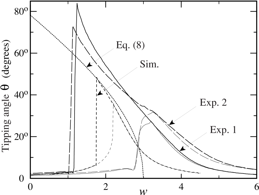
FIG. 4.: Tipping angle $\theta$ as a function of the normalized frequency shift $w$: Comparison of Eq. (10) to the measurements of Fig. 1. A numerical solution is also shown with parameter values as in the experiment, except for $H_{\rm rf}=0.014\,$Oe, $T=0.95\,T_{c}$, $\dot{H}=0.02\,$Oe/s, and spatially homogeneous counterflow at 0.70 cm/s. Upward sweeps of the field are plotted with thick and downward sweeps with thin lines.

Numerical simulation.—We have supplemented the analytic description with direct numerical solution of the Leggett–Takagi equations, by calculating the response of the spin-dynamic variables in the time domain for the spatially homogenous case during continuous rf excitation. Counterflow gives rise to the orientational energy Eq. (1) and to an additional torque, which contributes to Leggett–Takagi relaxation: $\vec{T}=\delta F_{\rm cf}/\delta\vec{\theta}$, where $\delta\vec{\theta}$ is an infinitesimal 3-dimensional rotation in spin space. The experimental parameters $(T,P,H,\dot{H},H_{\rm rf},\Omega)$ are adjusted to match the experimental conditions. A typical result is shown in Fig. 4. It agrees surprisingly closely with Eq. (10), demonstrating that the effects from relaxation and rf irradiation to the frequency shift are small. It also reproduces the shape of the measured NMR response, showing that the main difficulty in the comparison is the shift of the measured data to a higher temperature. In general, the simulation result is found to move closer to Eq. (10), when $T$, $H_{\rm rf}$, or $\Omega$ are increased. These are all changes, which help to boost either the value of $u$ or improve the compensation for relaxation, and thus enhance the stability of the new mode towards larger fields during the field sweep.

In conclusion, we have observed a highly nonlinear NMR response of ³He-B when the direction of the orbital momentum is fixed by large counterflow. This new state of precession has been identified as a Brinkman–Smith mode in a general classification scheme of states with fixed direction of $\vec{L}$. Other branches of the phase diagram can perhaps be found in experiments where the direction of $\vec{L}$ is fixed with solid walls or by tilting the magnetic field towards the flow direction.

REFERENCES

- [1]
- [2] W.F. Brinkman, H. Smith, Phys. Lett.51 A, 449 (1975).
- [3] W.F. Brinkman, H. Smith, Phys. Lett. 53 A, 43 (1975).
- [4] D.D. Osheroff and L.R.Corruccini, Phys. Lett. 51 A, 447 (1975); in Proc. 14th Intern. Conf. Low Temp. Phys. LT-14 Vol.1 (North-Holland, Amsterdam, 1975), p. 100.
- [5] See review by Yu.M. Bunkov, in Prog. Low Temp. Phys. Vol. XIV (Elsevier Science, Amsterdam, 1995), p. 69.
- [6] V.V. Dmitriev et al., Phys. Rev. Lett. 78, 86 (1997).
- [7] G. Kharadze et al., J. Low Temp: Phys. 110, 851 (1997).
- [8] S. Coleman, Nucl. Phys. B262, 263 (1985); more recent eg. A. Kusenko et al., Phys. Rev. Lett. 80, 3185 (1998).
- [9] See eg. P.J. Hakonen et al., J. Low Temp. Phys. 76, 225 (1989), and references therein.
- [10] V.M. Ruutu et al., J. Low Temp. Phys. 107, 93 (1997).
- [11] J.S. Korhonen et al., Phys. Rev. Lett. 65, 1211 (1990).
- [12] J.S. Korhonen et al., Phys. Rev. B46, 13983 (1992).
- [13] J.S. Korhonen, G.E. Volovik, JETP Lett. 55, 362 (1992). The time averaged dipole energy was first discussed by I.A. Fomin (J. Low Temp. Phys. 31, 509 (1978)).
- [14] Yu.M. Bunkov, G.E. Volovik, JETP 76, 794, (1993).