Coherent transport and nonlocality in mesoscopic SNS junctions: anomalous magnetic interference patterns

Victor Barzykin1,2 and Alexandre M. Zagoskin2 Email: zagoskin@physics.ubc.ca 1 National High Magnetic Field Laboratory, 1800 E. Paul Dirac Dr., Tallahassee, Florida 32310, USA;
2Physics and Astronomy Department, The University of British Columbia, 6224 Agricultural Rd., Vancouver, B.C., Canada V6T 1Z1
Abstract

We show that in ballistic mesoscopic SNS junctions the period of critical current vs. magnetic flux dependence (magnetic interference pattern), $I_{c}(\Phi)$, changes continuously and non-monotonically from $\Phi_{0}$ to $2\Phi_{0}$ as the length-to-width ratio of the junction grows, or temperature drops. In diffusive mesoscopic junctions the change is even more drastic, with the first zero of $I_{c}(\Phi)$ appearing at $3\Phi_{0}$.

The effect is a manifestation of nonlocal relation between the supercurrent density and superfluid velocity in the normal part of the system, with the characteristic scale $\xi_{T}=\hbar v_{F}/2\pi k_{B}T$ (ballistic limit) or $\tilde{\xi}_{T}=\sqrt{\hbar D/2\pi k_{B}T}$ (diffusive limit), the normal metal coherence length, and arises due to restriction of the quasiparticle phase space near the lateral boundaries of the junction. It explains the $2\Phi_{0}$-periodicity recently observed by Heida et al. (Phys. Rev. B 57, R5618 (1998)). We obtained explicit analytical expressions for the magnetic interference pattern for a junction with an arbitrary length-to-width ratio. Experiments are proposed to directly observe the $\Phi_{0}\to 2\Phi_{0}$- and $\Phi_{0}\to 3\Phi_{0}$-transitions.

It is well established that the electrodynamics of the superconductors is nonlocal on the scale of $\xi_{0}$ [1, 2], and so is the current-phase relation (since vector potential and superconducting phase both enter through one gauge-invariant combination, superfluid velocity). In the normal layer of an SNS system the place of $\xi_{0}$ is taken by the normal metal coherence length, $\xi_{T}=\hbar v_{F}/2\pi k_{B}T$ (in the ballistic limit, $L\ll l_{i}$, where $l_{i}$ is the impurity scattering length), or $\tilde{\xi}_{T}=\sqrt{D/2\pi k_{B}T}$, (in the diffusive limit, $l_{i}\ll L$) where $D=v_{F}l_{i}/3$ is the diffusion constant of electrons in the dirty metal [3, 4]. This length can obviously greatly exceed $\xi_{0}$ at low enough temperatures, and is limited only by the inelastic scattering length in the system, $l_{\phi}$, which also diverges as $T\to 0$. (The latter gives the scale of classical nonlocality in mesoscopic systems, related to formation of essentially nonequilibrium states, when currents are determined by potential drops far from the observation point, like in classical point contacts or Landauer wires.) In wide SNS junction, the nonlocality is responsible for the formation of current-carrying Andreev levels, formed in the normal part of the system by Andreev reflections of quasiparticles from the off-diagonal scattering potential (order parameter) of the superconducting banks [3, 4, 5], which provide the mechanism for the Josephson current flow. In mesoscopic SNS systems it is revealed in such effects as e.g. conductance oscillations in Andreev interferometers(Ref.[6] and references therein). It came nevertheless as a surprise, when Heida et al. [7] reported that the critical current vs. magnetic flux dependence (magnetic interference pattern) in mesoscopic junctions, formed by Nb electrodes in contact with 2D electron gas of InAs heterostructure (S-2DEG-S junction), has a period $2\Phi_{0}=hc/e$, instead of the standard $\Phi_{0}$ [8]. The authors of [7] posed a question whether this unexpected result is due to a nonlocal superconducting current-phase relation specific for their narrow (length-to-width ratio $L/W\sim 1$, instead of usual $L/W\ll 1$), ballistic, mesoscopic junction. They also asked whether the diffusive character of scattering at NS boundaries (which was prominent in the experimental samples) is important for establishing such nonlocality. A heuristic formula proposed in [7] successfully reproduced the periodicity, but not the shape of the observed magnetic interference pattern.

Since the nonlocality under question is already present in wide SNS junctions, where the magnetic interference pattern is nevertheless $\Phi_{0}$-periodic, the problem clearly requires a more thorough consideration. For example, the dephasing and inelastic scattering processes cannot be responsible for the ”wide-narrowβ€œ difference, because the standard theory [4, 9] predicts $\Phi_{0}$-periodicity even when $l_{\phi},\xi_{T}=\infty$.

In this paper we show that $\Phi_{0}\to 2\Phi_{0}$-transition is a size effect, resulting from the restrictions on allowed quasiclassical trajectories of quasiparticles in the normal layer near its lateral edges. It is present already in the absence of diffusive Andreev scattering (perfect NS boundaries). As the $L/W$ ratio drops, relative contributions from the edges diminish, and in the limit $L/W\to 0$ the standard $\Phi_{0}$-periodicity is restored. The latter is actually a result of certain contributions to the current cancelling each other, not of their decay because of junction size exceeding the inelastic scattering length. We also predict even more drastic effect in the diffusive SNS junction, that can be qualitatively explained along the same lines.

An important consequence of the ”geometricβ€œ origin of the effect is the continuous transition of the periodicity between Ξ¦0subscriptΞ¦0\Phi_{0} and 2​Φ02subscriptΞ¦02\Phi_{0} as the L/WπΏπ‘ŠL/W ratio changes. Indeed, the restriction on contributing quasiparticle trajectories can be considered as having a smaller effective flux through the system. The effective flux, and therefore the observed periodicity, obviously will be a continuous
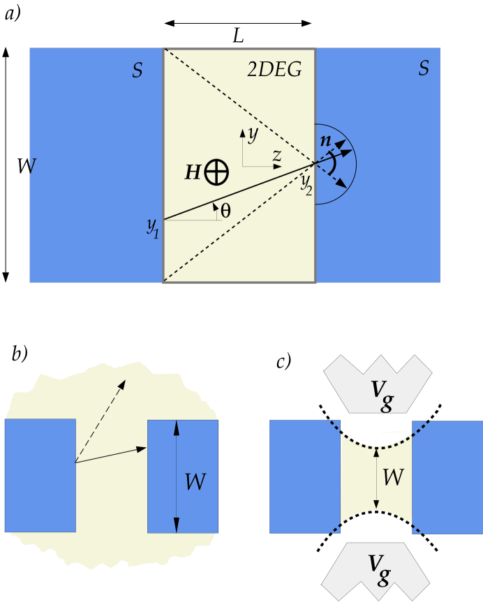
 function of L/WπΏπ‘ŠL/W. This transition could be directly observed in a modification of the experimental setup of [7], where the width of the channel is determined by the voltage applied to gate electrodes (Fig.1c). Such split-gate technique is now widely used in hybrid systems 2DEG-superconductor (see e.g. [10]). Another experimental possibility, applicable to the junctions of fixed dimensions (like in [7]), will be discussed later.

First consider a ballistic S-2DEG-S junction (Fig.1a) in the limit $L\gg\xi_{0}$, assuming perfect Andreev reflections at NS interfaces, and totally absorbing lateral boundaries (at $y=\pm W/2$). The latter condition, strictly speaking, corresponds to an ”open” SNS junction (Fig.1b), analogous to the structures investigated experimentally in [11]. In case of laterally restricted 2DEG one should use, e.g., condition of mirror reflection from the side walls. We will see that this does not qualitatively change the results.

The magnetic field and the vector potential (in the Landau gauge) are

$\displaystyle{\bf H}=H\hat{\bf x},\>\>\>{\bf A}=Hy\hat{\bf z}.$ (1)

Finally, we use the standard steplike approximation for the superconducting order parameter in the banks of the junction:

$\displaystyle\Delta({\bf r})=|\Delta_{0}|e^{i\phi_{1}}\theta(-L/2-z)+|\Delta_{0}|e^{i\phi_{2}}\theta(z-L/2).$ (2)

(In the gauge (1) the superconducting phase is not affected by the field.)

The Fermi wavelength in the normal part of the system, $\lambda_{F}=h/p_{F}\>(\approx 0.1\>\mu$m), is small compared to all other length scales in the problem. This allows us to apply the method of quasiclassical Green’s functions integrated over energies [12],

$\displaystyle g_{\omega}({\bf n},{\bf r})=\frac{i}{\pi}\int_{-\infty}^{\infty}d\!\xi{\cal G}_{\omega}(\xi,{\bf n};{\bf r});\>\>\>f_{\omega}({\bf n},{\bf r})=-\frac{1}{\pi}\int_{-\infty}^{\infty}d\!\xi{\cal F}_{\omega}(\xi,{\bf n};{\bf r});$
$\displaystyle f_{\omega}^{+}({\bf n},{\bf r})=f_{\omega}(-{\bf n},{\bf r})^{*};$
$\displaystyle g_{\omega}({\bf n},{\bf r})^{2}+f_{\omega}({\bf n},{\bf r})f_{\omega}({\bf n},{\bf r})^{+}=1.$

Here ${\cal G}_{\omega}(\xi,{\bf n};{\bf r}),{\cal F}_{\omega}(\xi,{\bf n};{\bf r})$ are spatial Fourier transforms of normal and anomalous Gor’kov functions of arguments ${\bf x}_{1,2}={\bf r}\pm\delta{\bf r}$. The momentum canonically conjugated to $\delta{\bf r}$ is

$${\bf p}=\sqrt{2m^{*}\xi}{\bf n}.$$

The supercurrent density is then found as a sum over Matsubara frequencies,

$\displaystyle{\bf j}({\bf r})=-4\pi ie{\cal N}(0)v_{F}T\sum_{\omega>0}\left<{\bf n}g_{\omega}({\bf n},{\bf r})\right>=-4\pi ie{\cal N}(0)v_{F}T\sum_{\omega>0}\left<{\bf n}(g_{\omega}({\bf n},{\bf r})-g_{\omega}(-{\bf n},{\bf r}))\right>_{n_{z}>0};$ (3)

the angular brackets denote angular averaging over the Fermi surface.

Functions $g_{\omega},f_{\omega}$ satisfy the set of Eilenberger equations, that in the ballistic limit and in the absence of the field is[13]

$\displaystyle(2\omega+v_{F}{\bf n}\cdot\nabla)f_{\omega}({\bf n},{\bf r})=2\Delta({\bf r})g_{\omega}({\bf n},{\bf r});$ (4)
$\displaystyle v_{F}{\bf n}\cdot\nabla g_{\omega}({\bf n},{\bf r})=\Delta({\bf r})^{*}f_{\omega}({\bf n},{\bf r})-\Delta({\bf r})f_{\omega}^{+}({\bf n},{\bf r}).$ (5)

Its characteristics are straight lines, interpreted as quasiclassical trajectories of quasiparticles[13]. It should be solved in three regions: $z<-L/2,|z|<L/2,z>L/2$, using the limiting values in the bulk of left, right superconductor,

$\displaystyle f_{\omega}({\bf n},z=\mp\infty)=\frac{|\Delta_{0}|e^{i\phi_{1,2}}}{\sqrt{|\Delta_{0}|^{2}+\omega^{2}}};$ (6)
$\displaystyle g_{\omega}({\bf n},z=\mp\infty)=\frac{\omega}{\sqrt{|\Delta_{0}|^{2}+\omega^{2}}},$ (7)

and then matching solutions over the interfaces. Eventually, this will yield the standard sawtooth expression for the superconducting current density in an SNS junction[9, 5, 14], which we will write in the form [15] for a point at the right NS boundary:

$\displaystyle j_{z}({\bf r}=y_{2}\hat{\bf y}+(L/2)\hat{\bf z})=\int_{\cos\theta>0}d\!\theta\frac{ev_{F}\cos\theta}{\lambda_{F}W}\frac{2}{\pi}\sum_{k=1}^{\infty}(-1)^{k+1}\frac{L}{l_{T}(\theta)}\frac{\sin k(\phi_{1}-\phi_{2})}{\sinh\frac{kL}{l_{T}(\theta)}}.$ (8)

Here $l_{T}(\theta)=\frac{\hbar v_{F}\cos\theta}{2\pi k_{B}T}=\xi_{T}\cos\theta$.

In our assumptions (totally absorbing walls) the integration over $\theta$ must be limited to the directions within the angle shown in Fig.1, and the total Josephson current is written as

$\displaystyle I(\phi_{1}-\phi_{2})=\frac{ev_{F}}{W\lambda_{F}L}\int\int_{-W/2}^{W/2}\frac{dy_{1}dy_{2}}{\left[1+(\frac{y_{1}-y_{2}}{L})^{2}\right]^{3/2}}\frac{2}{\pi}\sum_{k=1}^{\infty}(-1)^{k+1}\frac{L}{l_{T}(\theta_{y_{1}-y_{2}})}\frac{\sin k(\phi_{1}-\phi_{2})}{\sinh\frac{kL}{l_{T}(\theta_{y_{1}-y_{2}})}}$ (9)

(we take into account that $\tan\theta_{y_{1}-y_{2}}=(y_{2}-y_{1})/L$).

The only difference that nonzero magnetic field will make is that $(\phi_{1}-\phi_{2})$ in (8) will be replaced by

$\displaystyle\varphi({\bf n},{\bf r})=\phi_{2}-\phi_{1}+\frac{2\pi}{\Phi_{0}}\int^{0}_{\tau_{1}}{\bf A}({\bf r}-v_{F}\tau{\bf n})\cdot{\bf n}d\tau,$ (10)

where the vector potential is integrated along the quasiclassical trajectory. (We neglect here the dynamical effects of the magnetic field, small by the parameter $\hbar\omega_{c}/\mu.$) The expression for the Josephson current becomes

$\displaystyle I(\phi)=\frac{ev_{F}}{W\lambda_{F}L}\int\int_{-W/2}^{W/2}\frac{dy_{1}dy_{2}}{\left[1+(\frac{y_{1}-y_{2}}{L})^{2}\right]^{3/2}}\frac{2}{\pi}\sum_{k=1}^{\infty}(-1)^{k+1}\frac{L}{\xi_{T}\cos\theta_{y_{1}-y_{2}}}\frac{\sin k\left(\frac{\pi\Phi}{W\Phi_{0}}(y_{1}+y_{2})+\phi\right)}{\sinh\frac{kL}{\xi_{T}\cos\theta_{y_{1}-y_{2}}}};$ (11)
$\displaystyle I_{c}=\max_{0\leq\phi<2\pi}I(\phi).$ (12)

The current is given by a sum of the contributions from quasiclassical ”Andreev tubes” of width $\sim\lambda_{F}$ each, following the quasiparticle trajectories. Each contribution depends on the length of the trajectory, and on the phase gained along it (both from Andreev reflections at the NS boundaries, and from the vector potential on the way through the normal part of the system). You will also notice that heuristic formula (7) of Ref.[7] correctly captures the qualitative picture of the effect and follows from our expression in the limit of narrow junction at high temperature ($L/W,L/\xi_{T}\to\infty$).

At zero temperature, the results can be obtained explicitly in the limiting cases of wide ($L/W\to 0$) and narrow ($L/W\to\infty$) junctions. Introducing $\nu=\Phi/\Phi_{0},$ we obtain (see Fig.2)

$\displaystyle I_{c}(\nu)=\frac{2W}{\lambda_{F}}\frac{ev_{F}}{L}\frac{(1-\{\nu\})\{\nu\}}{|\nu|},\>\>L/W\to 0;$ (13)
$\displaystyle I_{c}(\nu)=\frac{W}{\lambda_{F}}\frac{ev_{F}}{L}\frac{(1-\{\nu/2\})^{2}\{\nu/2\}^{2}}{|\nu/2|^{2}},\>\>L/W\to\infty,$ (14)

where the first formula is the standard result for a wide SNS junction; all harmonics contribute to the current, producing the distinctly non-Fraunhofer picture [4, 9]. By $\{x\}$ we denote the fractional part of $x$.

In general case, the dependence $I_{c}(\nu)$ can be calculated numerically from (12) (see Fig.3). The period is indeed smoothly evolving from $\Phi_{0}$ to $2\Phi_{0}$. Near the wide limit we see almost uniform growth of the period, in agreement with our qualitative considerations, but in the intermediate regime, $L\sim W$, the behaviour of $I_{c}(\nu)$ becomes more complicated. It can be better understood in the high temperature limit, when only the term with $k=1$ in (11) survives. Then the answer can be obtained explicitly for an arbitrary value of $D=L/W$. Denoting by $D_{T}$ the ”effective aperture”,

$\displaystyle D_{T}=\frac{\sqrt{L\xi_{T}}}{W},$ (15)

we can write the expression for the critical current as

$\displaystyle I_{c}(\nu)=\frac{2^{5/2}ev_{F}}{\pi^{3/2}\lambda_{F}D_{T}}e^{-\frac{L}{\xi_{T}}}\left|f(\nu)\right|,$ (16)
$\displaystyle f(\nu)=\nu^{-1}e^{-\frac{\pi^{2}D_{T}^{2}\nu^{2}}{2}}{\rm Im}\left[e^{i\pi\nu}\left({\rm Erf}((1/D_{T}+i\pi D_{T}\nu)/\sqrt{2})-{\rm Erf}(i\pi D_{T}\nu/\sqrt{2})\right)\right].$ (17)

The function $f(\nu)$ is proportional to $\sin(\pi\nu)/\nu$ at $L/W=0$, and becomes strictly positive (proportional to $\sin^{2}(\pi\nu/2)/\nu^{2}$) as $L/W\to\infty$ (Fig.4). Thus the behaviour of $I_{c}(\nu)$ near its zeros shown in Fig.3 is due to merging of real roots of $f(\nu)$. We see from (16,17) that at finite temperature the ”wide-narrow” transition is governed by $\min(D_{T},L/W).$ Therefore another way of observation of the effect is by changing the temperature of the sample at fixed $L,W$. It has an advantage of being applicable to the mesoscopic SNS junctions of fixed dimensions.

What difference would make a different boundary condition in the lateral direction? In case of mirror reflection from the side walls the current is given by a simple generalization of (11), including the contributions from the reflected trajectories. In the absence of the magnetic field it is evident after we unfold the reflected trajectories by periodically extending the system in $y$-direction and taking the integral over $y_{1}$ from $-\infty$ to $\infty$, that the Josephson current per width $W$ of the contact will be the same as in an infinitely wide junction. But in the presence of the field the situation changes. Instead of linearly growing as $Hy$ (Eq.(1)), the effective vector potential in the extended system will be periodic in $y$[16], and the field contribution to the phase gain along the reflected trajectories will be systematically less than along their counterparts in an infinitely wide junction. Therefore the qualitative picture of the evolution of the oscillation period remains valid, as it is clearly seen in Fig.5.

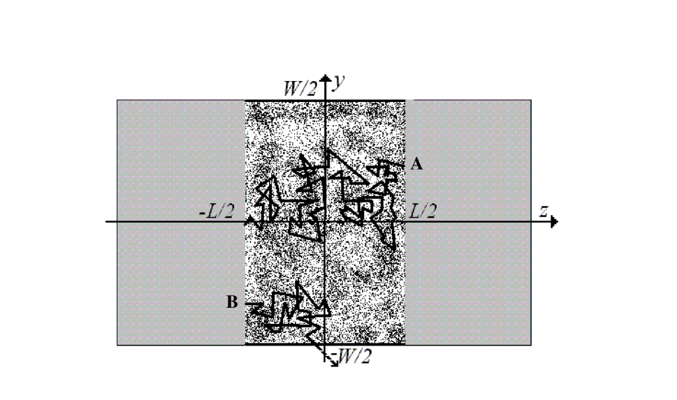
Effect of strong elastic scattering in the normal layer is more drastic. Let us consider the limiting case of dirty SNS junction (Fig.6). Now the system is described by the Usadel equations for the quasiclassical Green’s functions averaged over directions[17], $F_{\omega}$ and $G_{\omega}$. These equations and the expression for the supercurrent density read [4](from now on we put $\hbar=c=1$):

$\displaystyle|\omega|F_{\omega}({\bf r})+\frac{D}{2}\left(F_{\omega}({\bf r})\nabla^{2}G_{\omega}({\bf r})-G_{\omega}({\bf r})\left(\nabla+2ie{\bf A}({\bf r})\right)^{2}F_{\omega}({\bf r})\right)=\Delta^{*}({\bf r});$ (18)
$\displaystyle|F_{\omega}|^{2}+G_{\omega}^{2}=1;$ (19)
$\displaystyle{\bf j}({\bf r})=-\pi e{\cal N}(0)DT\sum_{\omega}{\tt Im}\left(F_{\omega}^{*}({\bf r})(\nabla+2ie{\bf A}({\bf r}))F_{\omega}({\bf r})\right).$ (20)

We will limit our considerations to long enough junctions and high enough temperatures, $L>\tilde{\xi}_{T}.$ Then the sum over Matsubara frequencies in (20) will be dominated by the terms with $|\omega|=\pi k_{B}T$; the anomalous Usadel function will be small inside the normal layer. Therefore the first Usadel equation can be linearized to yield

$$q_{T}^{2}F_{\omega}({\bf r})-\left(\nabla+2ie{\bf A}({\bf r})\right)^{2}F_{\omega}({\bf r})=0,$$ (21)

where $q_{T}^{2}=2|\omega|/D=1/\tilde{\xi}_{T}^{2}$. The boundary conditions for $F_{\omega}({\bf r})$ at $z=\pm L/2$ and $y=\pm W$ can be chosen as[4]

$$F_{\omega}(y,-L/2)=f_{0}(\omega);\>\>\>F_{\omega}(y,L/2)=f_{0}(\omega)e^{i(\phi_{2}-\phi_{1})},$$ (22)

where $f_{0}(\omega)=\Delta_{\pm L/2}/(|\omega|+\sqrt{|\omega|^{2}+\Delta_{\pm L/2}}).$ We are not interested in the actual value of the order parameter on the NS boundary (which due to proximity effect is lower than in the bulk), as long as the anomalous Green’s function stays small. We choose zero boundary conditions at $y=\pm W/2$, which would correspond to e.g. contact with clean normal conductor; the Josephson current is again carried only by the quasiparticles whose trajectories link the superconductors (Fig.6). After eliminating the vector potential from (20,21) by the transformation $F_{\omega}({\bf r})=\tilde{F}_{\omega}({\bf r})e^{-2ie{\bf A}{\bf r}}$, boundary conditions at $\pm L/2$ are modified:

$$\tilde{F}_{\omega}(y,-L/2)=f_{0}(\omega)e^{-i\pi\nu y};\>\>\>\tilde{F}_{\omega}(y,L/2)=f_{0}(\omega)e^{i(\phi_{2}-\phi_{1})}e^{i\pi\nu y}.$$ (23)

The solution is readily expressed through the Green’s function of Eq.(21), ${\cal G}(y,z;\eta,\zeta)$, in the rectangle with zero boundary conditions[18]:

$\displaystyle\tilde{F}_{\omega}(\eta,\zeta)=\frac{f_{0}(\omega)}{2\pi}\int_{-W/2}^{W/2}dy\left(e^{-i\pi\nu y}\left.\frac{\partial}{\partial z}{\cal G}(y,z;\eta,\zeta)\right|_{z=-L/2}-e^{i(\phi_{2}-\phi_{1})}e^{i\pi\nu y}\left.\frac{\partial}{\partial z}{\cal G}(y,z;\eta,\zeta)\right|_{z=L/2}\right).$

The latter can be found by the method of mirror images:

$${\cal G}(y,z;\eta,\zeta)=\sum_{m=-\infty}^{\infty}\sum_{n=-\infty}^{\infty}(-1)^{m}(-1)^{n}{\cal G}^{0}(mW+(-1)^{m}y,nL+(-1)^{n}z;\eta,\zeta).$$ (24)

Here ${\cal G}^{0}(y,z;\eta,\zeta)=\frac{1}{2\pi}K_{0}(q_{T}\sqrt{(y-\eta)^{2}+(z-\zeta)^{2}})$ is the Green’s function in the infinite plane, $K_{0}$ is the modified Bessel function.

Summation over $m$ can be limited to $m=0,\pm 1$ because of our assumption $L>\tilde{\xi}_{T}$. The sum over $n$ is taken using the Poisson summation formula. Substituting this in the expression for the current density at $z=0$, we finally find for the Josephson current:

$$I(\phi_{2}-\phi_{1},\nu)=I_{c}(\nu)\sin(\phi_{2}-\phi_{1}),$$

where

$\displaystyle I_{c}(\nu)=\pi e{\cal N}(0)DT|f_{0}|^{2}\left|f_{diff}(\nu)\right|,$ (25)
$\displaystyle f_{diff}(\nu)=\sum_{l=-\infty}^{\infty}(-1)^{l}S_{l}(L/2)S_{l}^{\prime}(L/2)\left(\frac{\sin\pi(\nu+l)/2}{\pi(\nu+l)/2}-(-1)^{l}\frac{\sin\pi(\nu-l)/2}{\pi(\nu-l)/2}\right)^{2},$ (26)
$\displaystyle S_{l}(u)=\sqrt{|u|/2\pi}(q_{T}^{2}+\pi^{2}l^{2}/W^{2})^{1/4}K_{1/2}(\sqrt{u^{2}(q_{T}^{2}+\pi^{2}l^{2}/W^{2})});\>\>\>S_{l}^{\prime}(u)=\frac{d}{du}S_{l}(u).$ (27)

Behaviour of the function $f_{diff}(\nu)$ is shown in Fig.7. Due to exponential decay of $S_{l}(L/2)$ and its derivative, in the limit of narrow junction ($W\ll\tilde{\xi}_{T},L$) only the terms with smallest $l=\pm 1$ survive[19]. This yields $f_{diff}(\nu)/f_{diff}(0)=\cos^{2}(\pi\nu/2)/(1-\nu^{2})^{2}$. The first zero of this function is at $\Phi=3\Phi_{0}$, tripling the first oscillation period. The following zeros are separated by $2\Phi_{0}$-intervals (though the amplitude of higher-order peaks decreases so fast with $\nu$, that the possibility to observe this periodicity is rather problematic). In the opposite limit of wide junctions, $W\gg\tilde{\xi}_{T},$ $S_{l}$’s cease to depend on $l$, and the shape of the interference pattern will be given by

$$\sum_{l=-\infty}^{\infty}(-1)^{l}\left(\frac{\sin\pi(\nu+l)/2}{\pi(\nu+l)/2}-(-1)^{l}\frac{\sin\pi(\nu-l)/2}{\pi(\nu-l)/2}\right)^{2}\equiv-4\frac{\sin\pi\nu}{\pi\nu},$$

the Fraunhofer pattern expected in a wide dirty SNS junction. As in the ballistic case, continious change of the periodicity can be caused by lowering the temperature of the system.

Note that in the range of parameters $(W\sim L\sim\tilde{\xi}_{T})$ when the first zero of the critical current appears at $\nu\sim 2$ the curve $I_{c}(\nu)(\propto|f_{diff}(\nu)|)$ is distinctly sharper than in the ballistic case (see Figs.4,7). Since the measurements of Ref.[7] (with diffusive scattering at NS boundaries) produced sharp cusps rather than smooth minima at $\Phi\sim 2\Phi_{0}$, one can speculate that their system was effectively in diffusive rather than ballistic regime.

Qualitatively the effect can also be understood in terms of loss of available phase space for current-carrying quasiparticles. Only the diffusive trajectories linking both superconductors contribute to the Josephson current (carried along such a trajectory by electrons and holes related through Andreev reflections at the end points). Therefore the trajectories originating too close to the lateral boundaries have more chances to end on the boundary and be lost, and the effective width of the junction, as well as the effective magnetic flux through it, are less than their actual values. Finite width of the junction also limits the ”wandering” trajectories with large effective phase gain. Due to strong elastic scattering, the average $z$-component of the current carried through such a trajectory is the same as for a ”shortcut” one, quite unlike the ballistic case where contributions from ”grazing” trajectories are systematically less. This explains why the periodicity change is even more drastic in the diffusive case.

In conclusion, we have demonstrated that the periodicity of the critical current dependence on the magnetic flux penetrating a mesoscopic SNS junction generally depends on the geometry of the system and is not given by either of fundamental quanta, $\Phi_{0}=hc/2e$ or $2\Phi_{0}=hc/e$, in a contrast to the case of tunneling Josephson junction. The effect is a manifestation of the nonlocal electrodynamics in hybrid normal-superconducting systems on scale $\xi_{T}(\tilde{\xi}_{T})\gg\xi_{0}$. It can be understood in terms of quasiclassical Andreev levels (”Andreev tubes”), following the quasiparticle trajectories in the normal part of the system. Our theory provides an explanation for the recent experimental observation of $2\Phi_{0}$-periodic magnetic interference pattern in S-2DEG-S junctions [7], and predicts a continuous transition from $\Phi_{0}$ to $2\Phi_{0}$ periodicity in ballistic case, and to $2\Phi_{0}$-periodicity with the first iscillation period $3\Phi_{0}$ on the dirty limit. This transition can be observed either by changing the width of the 2DEG layer in the split-gate technique, or by changing the temperature of the fixed-size junction. The latter approach can be applied as well to mesoscopic SNS junctions with normal metal layer instead of 2DEG.

We wish to thank I. Affleck, J.-S. Caux, L.P. Gor’kov, U. Ledermann, and P.C.E. Stamp for valuable discussions. This work was supported by NSERC of Canada and in part by CIAR (AZ) and by the NHMFL through NSF cooperative agreement No. DMR-9527035 and the State of Florida (VB).

REFERENCES

  • [1] A.B.Β Pippard, Proc. Roy. Soc. London, Swr. A, 216, 547 (1953).
  • [2] A.A.Β Abrikosov, L.P.Β Gorkov, and I.E.Β Dzyaloshinski, Methods of quantum field theory in statistical physics. New York: Dover Publications (1975). Ch.Β 7.
  • [3] I.O.Β Kulik, Sov. Phys. - JETP 30, 944 (1970).
  • [4] A.V.Β Svidzinskii, Spatially inhomogeneous problems in the theory of superconductivity. Nauka: Moscow (1982).
  • [5] J.Β Bardeen and J.L.Β Johnson, Phys. Rev. B 5, 72 (1972).
  • [6] H.A.Β Blom, A.Β Kadigrobov, A.M.Β Zagoskin, R.I.Β Shekhter, and M.Β Jonson , Phys. Rev. B 57, 9995 (1998).
  • [7] J.P. Heida, B.J. van Wees, T.M. Klapwijk, and G.Β Borghs, Phys. Rev. B 57, R5618 (1998).
  • [8] A.Β Barone and G.Β PaternΓ³, Physics and applications of the Josephson effect. New York: Wiley (1982).
  • [9] T.N.Β Antsygina, E.N.Β Bratus’, and A.V.Β Svidzinskii, Sov. J. Low Temp. Phys. 1, 23 (1975).
  • [10] H.Β Takayanagi, T.Β Akazaki, and J.Β Nitta, Surf. Sci. 361-362, 298 (1996).
  • [11] A.Β Dimoulas, J.P.Β Heida, B.J.Β van Wees, T.M.Β Klapwijk, W. v.d.Β Graaf, and G.Β Borghs, Phys. Rev. Lett. 74, 602 (1995).
  • [12] G. Eilenberger, Z. Phys. 214, 195 (1968).
  • [13] I.O.Β Kulik and A.N.Β Omelyanchuk, Sov. J. Low Temp. Phys. 4, 142 (1978).
  • [14] G.Β Ishii, Progr. Theor. Phys. 44, 1525 (1970).
  • [15] A.M.Β Zagoskin, J. Phys.: Condensed Matter 9, L419 (1997).
  • [16] Obviously, ${\bf A}_{eff}(y)=\hat{\bf z}HW(-1)^{q}(y/W-q)$ for $q-1/2\leq y/W\leq q+1/2;q=0,\pm 1,\dots.$
  • [17] K.Β Usadel, Phys. Rev. Lett. 25, 507 (1970).
  • [18] E.Β Madelung, Die Mathematischen Hilfsmittel des Physikers, Springer-Verlag, Berlin etc., 1957, X.D.3.
  • [19] Contributions from the terms with higher Matsubara frequencies in (20) would contain multiples of $q_{T}$ and are therefore exponentially small compared to the main contribution.
Refer to caption
FIG. 1.: (a) Josephson current in a ballistic S-2DEG-S junction. (b) ”Open” SNS junction. Only the quasiparticle trajectories linking both superconductors contribute to the Josephson current. (c) Suggested experiment for direct observation of the $\Phi_{0}\to 2\Phi_{0}$-transition. The width of the system is changed continuously by the gate voltage, $V_{g}$.
Refer to caption
FIG. 2.: Magnetic interference pattern at $T=0$ in wide ($L/W\to 0$) and narrow ($L/W\to\infty$) ballistic mesoscopic SNS junctions; $\nu=\Phi/\Phi_{0}.$
Refer to caption
FIG. 3.: Magnetic interference pattern and positions of zeros of the critical current as a function of length-to-width ratio (at $L=5\xi_{T}$). Note the nonmonotonic behaviour of even zeros, and the fact that exact $\Phi_{0}$- or $2\Phi_{0}$- periodicity takes place only in the limiting cases of infinitely wide (narrow) junction.
Refer to caption
FIG. 4.: Function $f(\nu)/f(0)$ at different values of $D_{T}=\sqrt{L\xi_{T}}/W$. The critical current $I_{c}(\nu)\propto|f(\nu)|.$ Changing the temperature of the system of fixed size will lead to evolution of the magnetic interference pattern.
Refer to caption
FIG. 5.: Magnetic interference pattern at $L=5\xi_{T}$ in case of total absorption (solid line) and mirror reflection (dots) from the side walls. The curves with different $D=L/W$ are offset in vertical direction.
Refer to caption
FIG. 6.: Josephson current in an SNS junction in diffusive limit. Trajectory A does contribute to the Josephson current, trajectory B does not.
Refer to caption
FIG. 7.: Function $f_{diff}(\nu)/f_{diff}(0)$ at $L=2\tilde{\xi}_{T}$ and different values of $W/\tilde{\xi}_{T}=0.5;1;2;3$ (dots). Solid lines show the limiting cases, $\cos^{2}(\pi\nu/2)/(1-\nu^{2})^{2}$ and $\sin(\pi\nu)/(\pi\nu)$ respectively. The critical current in a dirty SNS junction $I_{c}(\nu)\propto|f_{diff}(\nu)|.$