Origin of synchronized traffic flow on highways and its dynamic phase transitions

Abstract

We study the traffic flow on a highway with ramps through numerical simulations of a hydrodynamic traffic flow model. It is found that the presence of the external vehicle flux through ramps generates a new state of recurring humps (RH). This novel dynamic state is characterized by temporal oscillations of the vehicle density and velocity which are localized near ramps, and found to be the origin of the synchronized traffic flow reported recently [PRL 79, 4030 (1997)]. We also argue that the dynamic phase transitions between the free flow and the RH state can be interpreted as a subcritical Hopf bifurcation.

Experiences show that traffic flow has complicated properties. The fact that automobile is one of main transportation tools raises the traffic flow as one of the most important problems for engineers [1]. For physicists, on the other hand, traffic flow is an interesting many-body problem of interacting vehicles. Numerous experimental measurements revealed that traffic flow possesses qualitatively distinct dynamic states [2]. In particular, three distinct dynamic phases are observed in highways [3]: the free traffic flow which is analogous to laminar flow in fluid systems, the traffic jam state where vehicles almost do not move, and the synchronized traffic flow which is characterized by complicated temporal variations of the vehicle density and velocity.

Paralleled with experiments, many physical models have been proposed [4]. Cellular automaton models [5] have been developed which simulate each individual vehicle, and hydrodynamic models [6, 7] which provide macroscopic description of traffic flow. Subsequent studies [8, 9] of the models have explained many observed features of the free flow and traffic jams in highways. However, no satisfactory explanation for the synchronized flow is available to our knowledge.

Recently, Kerner and Rehborn reported analysis of systematic measurements performed on German highways. As one of main results, it was pointed out that the synchronized flow is spatially localized near ramps on highways [10]. This observation motivated us to explore in this paper effects of ramps on highway traffic flow. Through numerical simulations of a hydrodynamic model, we find that the presence of ramps generates a new kind of traffic states which becomes a spatially localized limit cycle of highway traffic flow under the constant external flux. We examine properties of the novel state and show that it is the origin of the synchronized flow.

In this work, we adopt the hydrodynamic model of highway traffic flow proposed by Kerner and Konhäuser [6], where the dynamic evolution is described by the Navier-Stokes-type equation of motion,

$$\rho\left({\partial v\over\partial t}+v{\partial v\over\partial x}\right)={\rho\over\tau}(V(\rho)-v)-c^{2}_{0}\ {\partial\rho\over\partial x}+\mu{\partial^{2}v\over\partial x^{2}}\ .$$ (1)

Here $\rho(x,t)$ is the local vehicle density, $v(x,t)$ the local velocity, $V(\rho)$ the safe velocity that is achieved in the time-independent and homogeneous traffic flow, and $\tau,c_{0},\mu$ are appropriate constants. Eq. (1) is paired with the modified equation of continuity [11],

$${\partial\rho\over\partial t}+{\partial(\rho v)\over\partial x}=q_{in}(t)\varphi(x-x_{in})-q_{out}(t)\varphi(x-x_{out})\,,$$ (2)

where the source and the drain terms on the right hand side represent the external flux through an on-ramp and through an off-ramp, respectively [12]. Here $\varphi(x)$, describing the spatial distribution of the external flux, is localized near $x=0$ and normalized so that $q_{in}(t)$ ($q_{out}(t)$) represents the total incoming (outgoing) flux.

To study effects of a single ramp, two ramps [13] are separated by a large distance $(|x_{in}-x_{out}|=L/2$ where $L$ is the system size) and numerical simulations are performed with periodic boundary conditions. The two-step Lax-Wendroff scheme is adopted as the main simulation scheme, and its reliability is verified through comparison with an alternative scheme: the classical fourth-order Runge-Kutta scheme applied to the time and the centered Euler scheme to the space [14]. Simulations are carried out for many different sets of parameters and qualitatively the same results are obtained. So for definiteness, we present results only for the following choice of parameters : $\tau=$ 0.5 min, $\mu=$ 600 km/h, $c_{0}=54$ km/h, and $V(\rho)=V_{0}(1-\rho/\hat{\rho})/(1+E(\rho/\hat{\rho})^{\theta})$ where the maximum density $\hat{\rho}=$ 140 vehicles/km, $V_{0}=120$ km/h, $E=100$, and $\theta=4$ [15]. Concerning the discretization, spatial intervals of $\Delta x=37.8$ m and time intervals of $\Delta t=10^{-4}$ min are found to be suitable. We choose the spatial distribution of the external flux as $\varphi(x)=(2\pi\sigma^{2})^{-1/2}\exp{(-x^{2}/{2\sigma^{2}})}$ with $\sigma=56.7$ m.

This model (1,2) was investigated previously [11] for the constant external flux $q_{in}(t)=q_{out}(t)=f$. For small $f$, it was found that an initially homogeneous flow $\rho(x,0)=\rho_{h}$, $v(x,0)=V(\rho_{h})$ evolves to slightly modified free flow where homogeneous regions with different densities are separated by narrow density-rising (or descending) regions near the ramps, the so-called transition layers. In contrast, for $f$ larger than a critical value, a local avalanche-like process occurs at the transition layer and traffic jam appears spontaneously. This study, however, failed to probe the synchronized traffic flow.

To find a clue to the missing third phase in traffic flow, we pay attention to the experimental observation [10] that for a range of $f$, traffic flow can be either in the synchronized flow or in the free flow. This bi-stability suggests that the transition from one locally stable state to the other may require some triggering events. So in our simulations, we apply a pulse-type perturbation with a finite amplitude. Specifically we first prepare a transition layer by applying the constant external flux $f$ which is below the critical point $f_{c}$ (for $f>f_{c}$, the stable free flow does not exist). Then a pulse of additional flux $\delta q_{in}$ is applied at the on-ramp for a short duration $\delta t$. As a result, a localized oscillating state appears from the free flow [16] (Fig. 1).

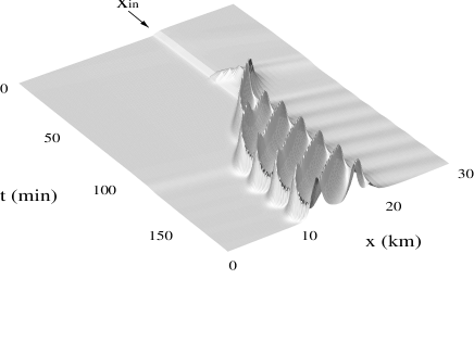
FIG. 1.: Birth and evolution of the RH state from the free flow is shown in this plot of the density profile ($\rho-\rho_{upstream}$) near the on-ramp ($x_{in}$=18.9 km) for the average density of the system $\rho_{h}$=22.4 vehicles/km $(\approx(\rho_{upstream}+\rho_{downstream})/2)$ and the constant external flux $f=318$ vehicles/h (the system size $L=75.6$ km). Transition from the free flow to the RH state is triggered by a pulse-type perturbation applied at $t=50$ min with $\delta q_{in}$=318 vehicles/h, $\delta t=5$ min.

After a transient period, the localized oscillation becomes periodic in time. We observe that the Fourier spectrum of the oscillation shows sharp peaks at each integer multiple of the basic frequency $1/T$ ($\approx 0.068$ min^-1 in case of Fig. 1). In the simulation, it turns out that properties of this periodic asymptotic state, such as the period and the oscillation amplitude, are essentially independent of $\delta q_{in}$ and $\delta t$ as long as they are large enough to trigger the transition. This strongly suggests that the periodic oscillation is not a transient process with long decay time but a limit cycle of Eqs. (1,2). For definiteness, we call this state of traffic flow the recurring hump (RH) state in this paper, which will be later compared with the synchronized flow.

Limit cycles are generated in numerous examples of nonlinear autonomous systems (that is, systems without explicitly given time dependence) [17, 18]. In the present example of traffic flow, the limit cycle can be characterized as a self-excited (autocatalytic) oscillator (see Sec. 5.6 in Ref. [17]), where constant external flux serves as a source of periodically generated excitations (humps). Excitations are, however, relaxed within a localized region. When the upstream vehicle density is lower than the critical value $\rho_{cr}(\approx 25$ vehicles/km for our parameter choice), a localized inhomogeneity decays away in the homogeneous traffic environment unless the amplitude of the inhomogeneity is larger than a critical magnitude [9]. Thus humps cannot survive far away from the on-ramp if its size does not exceed the critical magnitude. In this way, the localization can be achieved.

The character of the localized oscillation becomes evident in the density-flow diagrams ($\rho(x,t)$ vs.$q(x,t)\equiv$ $\rho(x,t)$$v(x,t)$). In contrast to a straight line for the free flow, the density-flow relation for the RH state forms a closed loop at $x=x_{in}$ (Fig. 2(a)), which implies the periodicity of the oscillation and also the phase difference in oscillation between $\rho(x,t)$ and $q(x,t)$. As $x$ moves downstream, the loop deforms gradually to a smaller loop and eventually joins the free flow (Fig. 2(a)), which is a consequence of the localization. We also examine the effect of randomly fluctuating external flux. Figure 2(b) shows that though the exact periodicity is lost, the oscillation itself is still stable under random fluctuations.

Below we investigate the transition from the free flow to the RH state. For definiteness, we fix the perturbation, $\delta q_{in}=159$ vehicles/h, $\delta t=6$ min and apply it to the transition layer generated by $f$ (Fig. 3(a)). For small $f$, the free flow survives the perturbation. For $f$ larger than a critical value $f_{1}$, however, the finite-amplitude RH state is induced. We emphasize that a finite perturbation is essential for the transition. As the perturbation becomes weaker, $f_{1}$ becomes larger and for $\delta q_{in}\delta t\rightarrow 0$, the transition to the RH state does not occur for the whole range of $f$ smaller than $f_{c}$ [11]. For the backward transition, on the other hand, it turns out that it may occur even without finite amplitude perturbations. As $f$ decreases adiabatically from $f>f_{1}$, the amplitude of the RH state varies as in Figure 3(a). The system first follows its old path. Below $f=f_{1}$, however, the system still remains in the RH state instead of going back to the free flow. The RH state is maintained until $f$ reaches a lower critical value $f_{2}$, where the transition to the free flow occurs [19]. We mention that transitions between the RH state and the free flow show the same hysteresis as measured in highways [10]. The influence of the transition on traffic flow becomes clear in the following natural order parameter: the spatio-temporal average velocity,

$$\langle v\rangle\equiv{1\over TR}\int_{t}^{t+T}dt^{\prime}\int_{-R/2}^{R/2}dx\ v(x+x_{in},t^{\prime})\ ,$$ (3)

where $T$ is the period of the RH state and $R$ is the size of the averaging range. In Figure 3(b), $\langle v\rangle$ makes discontinuous jumps at the transition points $f_{1}$ and $f_{2}$ [20].

FIG. 2.: (a) Density-flow diagrams for the average density $\rho_{h}=22.4$ vehicles/km, $f=318$ vehicles/h measured at $x-x_{in}=0$ km (the largest loop), $0.9$ km, and $3.8$ km (the smallest loop), respectively. The dashed line represents the free flow diagram. (b) Density-flow relation at the on-ramp under the presence of random fluctuations in the external flux. Data are shown for $q_{in,out}(t)=318$ vehicles/h $+\delta q_{in,out}(t)$ where $\delta q_{in,out}(t)$ is a random constant function in each time interval of $T_{p}=5$ min. At the end of each interval, the values of two independent random fluctuations $\delta q_{in}(t),\delta q_{out}(t)$ are reset by new random numbers uniformly distributed in the range $[-95,95]$ vehicles/h.

Another interesting property of the RH state appears in multi-lane situations. To demonstrate this, we extended the traffic equations to a two-lane system. The equation of motion (1) and the continuity equation (2) apply to each lane $i=1,2$. We assume that ramps are connected to the lane 2 and so the source and drain terms appear in the continuity equation for the lane 2 only. We simulate the inter-lane interaction effect in a minimal way by introducing to the continuity equations lane-change terms $(\partial\rho_{i}/\partial t)_{ch}$ that account for the inter-lane flux due to the lane change of vehicles. For the simple choice, $(\partial\rho_{i}/\partial t)_{ch}=a(\rho_{j}(x,t)-\rho_{i}(x,t))\ (i\neq j)$, it is found that when the flow in the lane 2 makes the transition to the RH state, it is accompanied by appearance of the synchronized oscillations of the velocity and the density in the lane 1 (Fig. 3(c)). This property of the synchronization is examined for different functional forms of $(\partial\rho_{i}/\partial t)_{ch}$ as well since its precise form is not well determined yet. Qualitatively same results are recovered in all cases, which demonstrates that the synchronization is a generic property of the RH state in multi-lane situations [21]. It is worth commenting that this kind of synchronization phenomena is a common property in many examples of self-exciting systems (see Sec. 5.13 in Ref. [17]).

Now it should be noticed that many properties of the RH state are identical to those of the synchronized flow [10], e.g., the discontinuous transition from the free flow to the synchronized flow induced by localized perturbations of finite amplitudes, hysteresis, stability of synchronized flow (hours of self-maintenance), gradual spatial transitions from synchronized flow to free flow, and synchronized oscillations. Therefore, we conclude that the RH state is the origin of the synchronized traffic flow.

FIG. 3.: (a) Amplitude of density oscillation measured at the on-ramp for $\rho_{h}=22.4$ vehicles/km. The zero amplitude implies free flow. Discontinuous jumps occur at $f_{1}\approx 241$ vehicles/h and $f_{2}\approx 184$ vehicles/h. (b) $\langle v\rangle$ (Eq. (3)) as a function of $f$ with $R=7.6$ km. Though the precise value of $\langle v\rangle$ depends on $R$, the presence of discontinuities is universal. (c) Synchronized oscillations in a two-lane system. The figure shows the temporal variations of the velocities at the on-ramp for the lane 1 (solid line) and for the lane 2 (dotted line). A pulse of the external flux introduced at $t=50$ min induced the transition to the RH state. Notice that the variations are synchronized in both lanes. (d) Schematic diagram of the bifurcation scenario. The point A corresponds to a turning point and B to a subcritical Hopf bifurcation point. While the transition at $f_{2}$ is spontaneous, the transition at $f_{1}$ should be aided by an external triggering event. As a result, the value of $f_{1}$ depends on the strength of triggering events. For $f>f_{c}$, the free flow loses its stability spontaneously.

We interpret our results within the standard framework of nonlinear dynamics. The free flow corresponds to a point attractor. On the other hand, many features of the RH state, such as stability and discontinuous transitions, assert that the RH state corresponds to a stable limit cycle. Hysteresis implies bi-stability for certain range of $f$. The spontaneous backward transition from the limit cycle to the point attractor means that the lower end of the bi-stable region is $f_{2}$. On the other hand, the necessity of finite perturbations for the forward transition suggests that the upper end of the bi-stable region goes above $f_{1}$ and in fact extends to $f_{c}$. Discontinuous transitions in both directions indicate that the limit cycle is not connected to the point attractor (Fig. 3(c)). The discontinuity also suggests that there should exist still another asymptotic state, which serves as a boundary between the basins of the attraction toward the two locally stable asymptotic states. One plausible candidate for the boundary is an unstable limit cycle that is connected to the stable limit cycle at $f=f_{2}$ and also to the fixed point at $f=f_{c}$ (Fig. 3(c)). In this case, the whole transition behaviors are results of a turning point ($f_{2}$) combined with a subcritical Hopf bifurcation ($f_{c}$).

Lastly we briefly discuss the synchronized flow far away from ramps reported in Refs.[3, 10]. There is one important difference between the synchronized flow near ramps and that far away from ramps. While the former is a non-decaying state of oscillations, the latter appears only as a transient process; after some upstream movement since its creation, it either disappears or transforms into a jam [10]. Therefore, the synchronized flow far away from ramps is not a stable dynamic phase of traffic flow, and is not studied in this paper. The appearance of this transient process requires further investigations.

In summary, we find that there exists recurring hump (RH) state in highway traffic flow with ramps. In this state, the density and the flow oscillate periodically and the oscillations are localized near the on-ramp. The RH state is a stable limit cycle of the nonlinear traffic equations (1,2). The transition between the free flow and the RH state is discontinuous and shows hysteresis. Many features of the RH state are identical to those of the synchronized flow and thus we conclude that the RH state is the origin of the synchronized flow observed in real highways [3, 10].

We acknowledge helpful discussions with Jysoo Lee, K. Chon, and M. Y. Choi. HYL thanks the Daewoo Foundation for financial support. This work is supported by the Korea Science and Engineering Foundation through the SRC program at SNU-CTP, and by the Ministry of Education through BSRI-97-2420.

REFERENCES

- [1] For example, see M. Wohl and B. V. Martin, Traffic System Analysis for Engineers and Planners (McGraw-Hill, New York, 1967); W. R. McShane and R. P. Roess, Traffic Engineering (Prentice Hall, Englewood Cliffs, N.J., 1990).
- [2] I. Treiterer and J. A. Myers, International Symposia on Transportation and Traffic flow, edited by D. J. Buckley (A. H. & A. W. Reed Pty Ltd., New South Wales, 1974); M. Koshi, M. Iwasaki, and I. Ohkura, in Proceedings of the Eighth International Symposium on Transportation and Traffic Theory, edited by V. F. Hurdle, E. Hauer, and G. N. Stewart (University of Toronto Press, Toronto, Ontario, 1983); E. E. Lee, Ph.D. Thesis, Civil engineering, Seoul National University, 1995.
- [3] B. S. Kerner and H. Rehborn, Phys. Rev. E 53, R4275 (1996).
- [4] For a review of traffic theory, see, for example, D. L. Gerlough and M. J. Huber, Traffic Flow Theory, Special Report No. 165 (Transportation Research Board, National Research Council, Washington, DC, 1975).
- [5] K. Nagel and M. Schreckenberg, J. Phys. I (France) 2, 2221 (1992).
- [6] B. S. Kerner and P. Konhäuser, Phys. Rev. E 48, R2335 (1993).
- [7] D. Helbing, Phys. Rev. E 51, 3164 (1995).
- [8] M. Schreckenberg, A. Schadschneider, K. Nagel, and N. Ito, Phys. Rev. E 51, 2939 (1995).
- [9] B. S. Kerner and P. Konhäuser, Phys. Rev. E 50, 54 (1994).
- [10] B. S. Kerner and H. Rehborn, Phys. Rev. Lett. 79, 4030 (1997).
- [11] B. S. Kerner, P. Konhäuser, and M. Schilke, Phys. Rev. E 51, 6243 (1995).
- [12] When an on-ramp and an off-ramp are closely positioned, and the influx through the on-ramp is much larger than the outflux through the off-ramp, this ramp pair can be treated as a single on-ramp.
- [13] With periodic boundary condition, the presence of the balanced off-ramp () is essential. Without it, the total vehicle number in the system varies with time, which prohibits investigation of asymptotic states.
- [14] W. H. Press, S. A. Teukolsky, W. T. Vetterling, and B. P. Flannery, Numerical Recipes in C (Cambridge University Press, Cambridge, 1992).
- [15] The form of is chosen so as to be consistent with available free flow data [10] and also with large density asymptotic behaviors. But its exact form is not important.
- [16] In Figure 1(a), the initial direction of the first hump movement varies depending on the parameter choice and the strength of the perturbation. For sufficiently large perturbations, however, the initial direction is toward upstream.
- [17] E. A. Jackson, Perspectives of Nonlinear Dynamics, Vol. 1 (Cambridge University Press, Cambridge, 1989).
- [18] For examples in hydrodynamic systems, see S. A. Orszag and L. C. Kells, J. Fluid Mech. 96, 159 (1980); S. A. Orszag and A. T. Patera, in Transition and Turbulence, ed. R. E. Meyer (Academic Press, London, 1981).
- [19] For very close to , oscillation patterns become complex with the exact periodicity lost. Currently, we do not know the precise origin of the complexity.
- [20] Such discontinuities cannot be detected in the spatio-temporal average flow , because the RH is connected to homogeneous regions, whose densities are essentially not altered by the appearance of the RH state if the system is sufficiently large, and hence the equation of continuity (2) forbids finite change in the average flow upon the infinitesimal change in .
- [21] H. Y. Lee, D. Kim, and M. Y. Choi, in Traffic and Granular Flow II, edited by D. E. Wolf and M. Schreckenberg, Springer, (1998); H. Y. Lee, H. -W. Lee, D. Kim, and M. Y. Choi, to be published.