rf-studies of vortex dynamics in isotropic type-II superconductors.

Abstract

We have measured the surface impedance of thick superconductors in the mixed state over a broad 2 kHz – 20 MHz frequency range. The depinning cross-over is observed; but it is much broader than expected from classical theories of pinning. A striking result is the existence of size effects which invalidate the common interpretation of the low-frequency surface inductance in terms of a single penetration depth. Instead, a two-mode description of vortex dynamics, assuming free vortex flow in the bulk and surface pinning, accounts quantitatively for the spectrum of the complex apparent penetration depth.

,

1 Introduction

The presence of an array of quantized vortices ($\psi\!=\!0$ lines) in a type-II superconductor entails a frictional force in the Euler equation for the supercurrent. For an isotropic material it takes the form [1]

$$\boldsymbol{E}+\frac{m}{e}\frac{\partial\boldsymbol{V}_{\!\!{\rm s}}}{\partial t}=\beta\boldsymbol{\omega}\times\left[(\boldsymbol{J}_{\!{\rm s}}+\text{curl}\,\boldsymbol{\varepsilon})\times\boldsymbol{\nu}\right]+\beta^{\prime}\boldsymbol{\omega}\times(\boldsymbol{J}_{\!{\rm s}}+\text{curl}\,\boldsymbol{\varepsilon})=\boldsymbol{\omega}\times\boldsymbol{v}_{\rm L},$$ (1)

where $\boldsymbol{V}_{\!\!{\rm s}}$, $\boldsymbol{J}_{\!{\rm s}}=-n_{\rm s}e\boldsymbol{V}_{\!\!{\rm s}}$ and $n_{\rm s}$ are coarse-grained mean values of the superfluid velocity, supercurrent, and density of superelectrons; $m$ and $e$ are the electronic mass and charge. The electric field $\boldsymbol{E}$ is directly related to the vortex field $\boldsymbol{\omega}=n_{\rm V}\varphi_{0}\boldsymbol{\nu}$ and the line velocity $\boldsymbol{v}_{\rm L}$ through the generalized Josephson equation. The vector $\boldsymbol{\omega}$ incorporates both density $n_{\rm V}$ and orientation $\boldsymbol{\nu}$ of the vortex lines.

The macroscopic London equation, [2, 3]

$$\boldsymbol{\omega}=\boldsymbol{B}-\frac{m}{e}\text{curl}\,\boldsymbol{V}_{\!\!{\rm s}}=\boldsymbol{B}+\text{curl}\,(\mu_{0}\lambda^{2}\boldsymbol{J}_{\!{\rm s}}),$$ (2)

shows that vortex lines may deviate from magnetic field lines ($\boldsymbol{\omega}\neq\boldsymbol{B}$) in the presence of a supercurrent. In Eq. (2) $\lambda$ is a field-dependent penetration depth.

Here we consider a slab in a perpendicular applied field $\boldsymbol{B}_{0}$. The vortex density $n_{\rm V}\simeq B_{0}/\varphi_{0}$ is nearly constant, but $\boldsymbol{\nu}$ may be quite different from $\boldsymbol{B}/B$; such bending effects are particularly important near the sample surface.

Eq. (1) is the superconducting analog of the acceleration equation for rotating superfluids (Eq.(24) in Ref. [4]) and has been written in its most general form such as deduced from conservation laws. The line tension $\boldsymbol{\varepsilon}=\varepsilon\boldsymbol{\nu}$ is the thermodynamic conjugate variable of $\boldsymbol{\omega}$. Kinetic coefficients $\beta$ and $\beta^{\prime}$ describing the longitudinal (resistive) and transverse (reactive) components of the friction force are analogs of the mutual friction parameters $B$ and $B^{\prime}$ in rotating superfluids [5, 6]. Allowing for a normal-current contribution $\boldsymbol{J}_{\!{\rm n}}=\bar{\sigma}\boldsymbol{E}$ ($\sigma=\bar{\sigma}_{\parallel},\sigma^{\prime}=\bar{\sigma}_{\perp}$) in the total current $\boldsymbol{J}\!=\!\boldsymbol{J}_{\!{\rm n}}\!+\!\boldsymbol{J}_{\!{\rm s}}$, $\beta$ is related to the longitudinal flux-flow conductivity $\sigma_{\rm f}\!=\!\sigma\!+\!1/\beta\omega$. The Hall-angle is related to $\beta^{\prime}$ through $\tan\theta_{H}\!=\!(\sigma^{\prime}\!+\!1/\beta^{\prime}\omega)/\sigma_{\rm f}$.

In conventional dirty superconductors dissipation ($\beta$) arises from normal-current back-flow and relaxation phenomena at the vortex core, while Hall angles are small. Of special interest for future experiments will be the case of clean superconductors at low temperatures where $\sigma_{\rm f}\simeq 1/\beta\omega$ and $\theta_{H}$ are expected to be governed by the discreteness of core levels in relation with the symmetry of the order parameter [7, 8].

Vortex dynamics is best probed by measuring the surface impedance $Z\!=\!R-{\rm i}X$ in the linear regime, which is conveniently expressed in terms of an effective complex penetration depth

$$\lambda_{\rm ac}=-\frac{Z}{{\rm i}\mu_{0}\Omega}=\lambda^{\prime}+{\rm i}\lambda^{\prime\prime}.$$ (3)

A perfect sample, completely free from defects, should behave like a continuous resistive medium with $Z=(1+{\rm i})\delta_{\rm f}/2$, where $\delta_{\rm f}=(2/\mu_{0}\sigma_{\rm f}\Omega)^{1/2}$ is the usual skin-depth. In real samples, this ideal response has been observed in conventional superconductors at microwave frequencies $\Omega/2\pi\sim 10$ GHz [9], and also for moving vortex arrays driven by a large superimposed dc transport current ($I\gg I_{\rm C}$) [10]. At low frequencies (and $I=0$) the linear ac response is strongly altered by pinning, so that a sample in the mixed state behaves as a true loss-free superconductor, with $\lambda^{\prime\prime}\simeq 0$ [11] and a quasistatic penetration depth $\lambda^{\prime}\sim$ 1–100 $\mu$m [12]. The way pinning and flux flow interfere in the cross-over regime ($\Omega/2\pi\sim$ 0.1–100 MHz in dirty conventional materials) is involved in the complex spectrum $Z(\Omega)$, which consequently should be the main concern for the dynamics of pinning (see the theoretical review [13] and references therein). From a practical point of view it is equally important to know the width of the cross-over regime and the position of its center point, the depinning-frequency $\Omega_{\rm p}$, because they determine both the onset of losses at low frequencies and the recovery of the free flux-flow response at high frequencies.

Our experiment is designed to study the skin-depth spectrum $\lambda_{\rm ac}(\Omega)$ in the cross-over regime. For this purpose, we measure the penetration of small rf magnetic fields into thick superconducting slabs in a large frequency range, $\Omega/2\pi\sim$ 2 kHz–20 MHz .

The quasistatic regime is classically described in terms of an elastic interaction between the vortex array and sample defects [14] (p.370). Assuming the existence of a pinning force density, small vortex displacements $\boldsymbol{u}$ about their equilibrium position result from a Lorentz force $\boldsymbol{J}\times\boldsymbol{\omega}$ per unit volume, balanced by a linear restoring force $\boldsymbol{F}_{\!{\rm p}}\!=\!-\alpha_{\rm L}\boldsymbol{u}$, where $\alpha_{\rm L}$ is the phenomenological Labusch parameter. With increasing frequency a viscous term $-\eta\boldsymbol{v}_{\rm L}$ ($\eta=\sigma_{\rm f}\omega^{2}$) comes into play and damps vortex motion. Linearizing both the Josephson relation $\boldsymbol{E}=\boldsymbol{\omega}\times\boldsymbol{v}_{\rm L}$ ($\boldsymbol{v}_{\rm L}=\dot{\boldsymbol{u}}$) and the force-balance equation, one obtains a local constitutive equation in the form of the Ohm’s law $\boldsymbol{J}_{\!\perp}=\sigma^{*}\boldsymbol{E}$, where $\sigma^{*}=\sigma_{\rm f}\!+\!{\rm i}\alpha_{\rm L}/(\omega^{2}\Omega)$. This results in a one-mode electrodynamics with a complex penetration depth $\lambda_{\rm ac}$ given by

$$\frac{1}{\lambda_{\rm ac}^{2}}=-{\rm i}\mu_{0}\sigma^{*}\Omega=\frac{1}{\lambda_{\rm C}^{2}}-\frac{2{\rm i}}{\delta_{\rm f}^{2}}.$$ (4)

Here $\lambda_{\rm C}=\omega/(\mu_{0}\alpha_{\rm L})^{1/2}$ is the Campbell penetration depth for small quasistatic vortex motions [12]. The spectrum (4) has been amended so as to include thermally-assisted vortex motion (flux creep) [15, 16]. Thermal activation entails an additional $\Omega$-dependence in $\alpha_{\rm L}$ (or $\lambda_{\rm C}$) at low frequencies, but it preserves the electrodynamic description in terms of a local effective conductivity $\sigma^{*}$ [13].

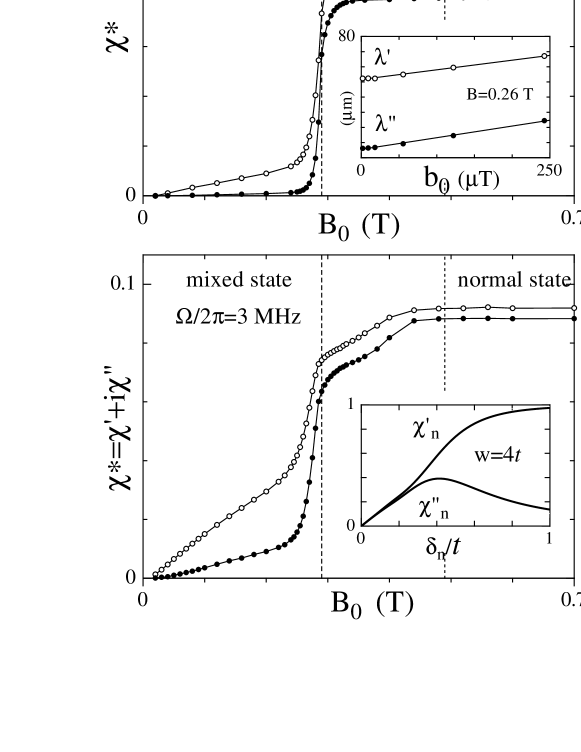
Figure 1: Transverse susceptibility of a $6.1(w)\times 1.22(t)$ mm² PbIn${10.5\%wt}.$ slab ($\rho_{\rm n}=10.3\,\mu\Omega$cm) in a broad range of normal fields including the mixed state ($B_{0}\leq 0.29\,$T) and the surface sheath regime ($0.29\,$T$\leq B_{0}\leq 0.49\,$T). The upper panel shows the quasistatic response at low frequency with vanishing losses ($\chi^{\prime\prime}$) and a finite in-phase apparent penetration depth $\lambda^{\prime}=\chi^{\prime}t/2$. In the lower panel, $\Omega$ is close to the depinning threshold $\Omega_{\rm p}$, and $\chi^{\prime\prime}$ is clearly visible. For each frequency, the normal state response (plateau for $B_{0}\geq 0.49\,$T) is used to calibrate the phase and the amplitude of the excitation by comparison with a two-dimensional calculation (inset of the lower panel and Eqs. (5)). Non-linear effects are displayed in the inset of the upper figure: strictly the linear response requires extrapolating data to $b_{0}=0$ for each field and frequency; in practice we work with a constant but small level $b_{0}\sim 1\,\mu$T (or induced currents $K=b_{0}/\mu_{0}\sim 10\,$mA/cm), which translates into minute vortex displacements $u\simeq\lambda^{\prime}b_{0}/B_{0}\sim 1$ Å.

According to a recent two-mode electrodynamics [17, 18], which follows from linearized Eqs. (1) and (2), there is, apart from the ordinary flux-flow mode (FF-mode), a second mode associated with strain and corresponding to $\text{curl}\,\boldsymbol{\varepsilon}$ terms in Eq. (1): this vortex-strain mode (VS-mode) is evanescent and non dissipative. It is worth noting that in Eq. (1) (like for superfluids in [4]) shear effects are disregarded. We adopt a rather old line of reasoning [19], according to which the small shear rigidity of the vortex array may be ignored in most dynamic problems. It remains that the shear modulus $c_{66}$ is essential for questions about the detailed equilibrium configuration of the vortex lattice; we return to this point in Sec. 6. On the other hand one cannot ignore the role of the VS-mode: although it dies off over a short depth $\lambda_{\rm V}\gtrsim a$ from the surface, it can carry large non-dissipative currents, $\boldsymbol{J}_{\!{\rm s}}=-\text{curl}\,\boldsymbol{\varepsilon}$ ($J_{\rm s}\lesssim\varepsilon/\lambda_{\rm V}\sim 10^{7}$ A/cm²). On introducing the appropriate surface condition for small reversible vortex motion, the amplitude and the phase of the two modes, and ultimately the surface impedance of the sample, are determined. It turns out that for the ac response of a perfect sample the surface condition $\boldsymbol{\nu}_{\parallel}=0$ applies, reducing the amplitude of the VS-mode to its (small) diamagnetic contribution [10]. However, as suggested recently [17, 20], the VS-mode can be considerably enhanced by surface roughness: surface irregularities on the scale of $a$ allow for an hysteresis in the “contact angle” between the vortex array and the averaged smoothed sample surface ($\nu_{\parallel}\lesssim 0.1$). On substituting the vortex slippage condition $\boldsymbol{\nu}_{\parallel}=-\boldsymbol{u}/l$, for the ideal boundary condition, we find a number of important results. The hallmark of the two-mode electrodynamics is the original shape of the $\lambda_{\rm ac}(\Omega)$ spectrum (see Eq. (14) and Figs. 2 and 3 below). Furthermore, we predict unexpected size-effects which are discussed in Sec. 5 and Fig. 6.

In this paper we detail the experimental procedure (Sec. 2), show new results on PbIn alloys over an extended frequency range both for perpendicular and oblique fields, and discuss finite-size effects at some length. A preliminary investigation of the sheath-superconductivity regime (above $B_{\rm C2}$), included in Sec. 4, supports our interpretation of the mixed-state spectra in term of two modes. The paper ends with a discussion about pinning mechanisms.

2 Experimental principle

We have investigated a series of long superconducting slabs (length $L$ in the $x$-direction, width $w$ in the $y$-direction). The applied magnetic field $B_{0}$, in the $yz$-plane, makes an angle $\theta$ with the $z$-direction. We concentrate to the $\theta=0$ and $\theta=\pi/4$ orientations referred to below as normal and oblique field. A small ac ripple $b_{0}e^{-i\Omega t}$ along the $x$-axis is produced by a 10–100 turns excitation coil. Induced currents make the vortices oscillate in the $xz$ planes. The ac flux $\Phi^{*}e^{-i\Omega t}$ through the cross-section $w\times t$ is detected by means of a 10–100 turns pick-up coil wound on the sample and measured with phase-sensitive lock-in analysers (EGG 5202 and 5302) in the broad $\Omega/2\pi=$2 kHz–20 MHz frequency range. In order to obtain a high resolution in the loss-angle $\varphi\!=\!\arctan(\lambda^{\prime\prime}/\lambda^{\prime})$ ($\delta\varphi\lesssim 0.3$ degree below 1 MHz) we used thin bronze wire to make pick-up coils transparent to the ac-field, and the rf chamber was enclosed in a high-conductivity copper can. At the low excitation levels of the linear regime ($b_{0}\lesssim 1\,\mu$T in Fig. 1), the resolution was ultimately limited to $\delta\lambda\lesssim 0.1\,\mu$m by electronic noise. Flux-flow conductivities and critical currents were measured beforehand from dc voltage-current characteristics ($I\leq 25$ A).

Most measurements reported in this paper were carried out on PbIn${10.5\%wt}$ slabs $40(L)\times 6(w)\times t$ mm³ with $t=0.3,1.3,4$ mm. Homogeneous lead-indium alloys are easily prepared from pure metals, and extensive measurements in the literature give reliable values of their $B_{\rm C2}$, $\kappa$ and $\rho_{\rm n}$ ($10.3\,\mu\Omega$cm) [21]. Slabs were spark-cut directly from ingots and optionally chemically etched. With $\kappa=3.5$ magnetization effects are negligible down to very low fields, and $\omega=B_{0}$. On the other hand, $B_{\rm C2}$ (0.29 T at 4.2 K) is low enough so that the field-phase diagram can be investigated up to the normal state with our 0.8 Tesla magnet (see Fig. 1). Measurements on very clean niobium ($\rho_{\rm n}\lesssim 10$ n$\Omega$cm), first reported in Ref. [20], will be detailed elsewhere. We show in Fig. 3 new data on PbIn${5\%wt}$ ($\rho_{\rm n}=6.5\,\mu\Omega$cm) and standard vanadium ($99.5\%$ with $\rho_{\rm n}=0.6\,\mu\Omega$cm), which exhibit the same behaviour as PbIn${10.5\%wt}$.

For the sake of obtaining absolute values of $\lambda_{\rm ac}$ we need to calibrate the ac-field $b_{0}$ accurately both in amplitude and phase. Several techniques can be used for this purpose: the phase can be obtained from that of the current in the rf excitation coil, or by measuring the magnetic flux either through an auxiliary pick-up coil, or through the gap between the pick-up coil and the sample in the Meissner state $B_{0}=0$. The Meissner state is used throughout this work as the reference $\Phi^{*}=0$ state, neglecting the penetration over the small London depth $\lambda_{\rm L}\sim 0.1\,\mu$m. The most accurate technique, however, makes use of the complex susceptibility of the normal state $\chi^{*}_{\rm n}$. Knowing $\rho_{\rm n}$, the flux distribution in an isotropic normal metal can be easily calculated thanks to the homogeneous boundary conditions achieved in this geometry. Note in this respect that the situation is far less tractable in resistivity experiments where the spatial distribution of the ac applied current is an intricate problem; moreover, the measured voltage strongly depends on the leads arrangement.

For a precise calibration of the phase of the exciting field in the normal state, we need the exact two-dimensional solution for the field distribution in a rectangular cross section $w\times t$, which reads :

$$\frac{b}{b_{0}}=\sum_{m,n\;{\rm odd}}\frac{16}{mn\pi^{2}}\frac{k_{mn}^{2}}{k_{mn}^{2}-2i/\delta_{\rm n}^{2}}\sin\frac{m\pi y}{w}\sin\frac{l\pi z}{t}$$

$$(k_{mn}^{2}=\frac{m^{2}\pi^{2}}{w^{2}}+\frac{n^{2}\pi^{2}}{t^{2}}).$$

Integration over the section yields the apparent susceptibility $\chi_{\rm n}^{*}=\Phi_{\rm n}^{*}/b_{0}wt$ :

$$\chi_{\rm n}^{*}=\sum_{m,n\;{\rm odd}}\;\frac{64}{m^{2}n^{2}\pi^{4}}\;\frac{k_{mn}^{2}}{k_{mn}^{2}-2i/\delta_{\rm n}^{2}}.$$ (5)

The inset in the lower Fig. 1 shows $\chi_{\rm n}^{\prime}$ and $\chi_{\rm n}^{\prime\prime}$ as a function of $\delta_{\rm n}/t\propto 1/\sqrt{\Omega}$, calculated from Eq. (5) for $w=4t$. As a cross check we always observed that the phase determined by other methods coincides with that obtained from the normal-state response within 0.3 degrees below 1 MHz. The calibration from the normal-state response is, for a large part, unaffected by stray capacitances from which coil circuits usually suffer at high frequencies.

Whereas a 2D calculation was necessary in the normal-state response, the situation is different in the mixed state because of the strong anisotropy of the critical currents and the flux flow resistivity. In particular, as can be checked experimentally by making $\theta=\pi/2$, the flux penetration through the lateral faces parallel to the vortices is negligible below $0.9B_{\rm C2}$. Flux penetration in normal field can thus be regarded as a one-dimensional problem with $\Phi^{*}=2wb_{0}\lambda_{\rm ac}$. Anyway, the question of the lateral penetration can be circumvented by working in oblique field where the 4 faces play symmetric roles so that $\Phi^{*}=2(w+t)b_{0}\lambda_{\rm ac}$. In oblique field, bulk currents flow at an angle $\theta=\pi/4$ with vortices, and the effective resistivity is $\rho_{\rm f}(\theta)=\rho_{{\rm f}\perp}\cos^{2}\theta$.

The experimental procedure is the following: the flux $\Phi^{*}\!=\!\Phi(B_{0})\!-\!\Phi(0)$ is measured as a function of $B_{0}$ at constant $\Omega$ up to the normal state where the calibration is achieved. Then the data for each vortex state are collected as a function of $\Omega$ to yield the complex spectrum. In PbIn${10.5\%wt}$ slabs the resolution was not affected by the reproducibility of the vortex states. Otherwise we are careful to reproduce the same vortex state, either by using the same field history or by removing metastability by applying a large transient over-critical dc current. The frequency-range is limited to two decades for a given arrangement of exciting and pick-up coils; it is extended to four decades in Figs. 2 and 3a by juxtaposing data taken from two distinct experimental setups with different windings, with several days lying between the two measurements.

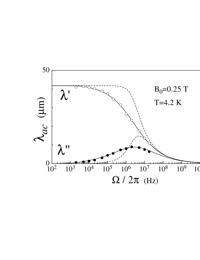
Figure 2: Broad-band spectrum of the apparent penetration depth $\lambda_{\rm ac}$ in a $6(w)\times 4(t)\,$mm² PbIn${10.5\%w}$ slab in oblique field. It shows the cross-over between the quasistatic regime ($\Omega/2\pi\lesssim 1$ kHz) and the free flux-flow regime ($\Omega/2\pi\gtrsim 1$ GHz). The 2 kHz–20 MHz experimental range has been achieved by using two different set-ups, each covering two frequency decades. Solid lines are theoretical fits to Eq. (14) with $L_{\rm S}=42\pm 0.5\,\mu$m and $\rho_{\rm f}=4.0\pm 0.1\,\mu\Omega$cm. For comparison the Campbell spectrum (4) (dashed-line), with the same set of parameters, yields a much narrower transition with a maximum $\lambda^{\prime\prime}/L_{\rm S}=0.272$ larger than the maximum $\lambda^{\prime\prime}/L_{\rm S}=0.207$ of the solid line.

3 Skin effect in the mixed state

Let us first recall the theoretical steps leading to the two-mode impedance spectrum (14), developed in Refs. [17, 18, 20].

Consider a superconducting half-space $z<0$, immersed in a constant magnetic field $B_{0}\hat{z}$, and submitted to a small transverse ripple $b_{0}\hat{x}e^{-i\Omega t}$. In the absence of Hall effects ($\beta^{\prime}=0$), vortex modes are linearly polarized, and the ac fields $b_{x},E_{y},\nu_{x},u=\nu_{x}/{\rm i}k$, …split into two modes,

$$b_{x} = \;b_{0}(\tilde{b}_{1}{\rm e}^{z/\lambda_{\rm f}}+\tilde{b}_{2}{\rm e}^{z/\lambda_{\rm V}})\;{\rm e}^{-{\rm i}\Omega t},$$ (6)

$$E_{y} = -b_{0}(\lambda_{\rm f}\tilde{b}_{1}{\rm e}^{z/\lambda_{\rm f}}+\lambda_{\rm V}\tilde{b}_{2}{\rm e}^{z/\lambda_{\rm V}})\;i\Omega{\rm e}^{-{\rm i}\Omega t},$$ (7)

$$\nu_{x} = \;(\nu_{1}{\rm e}^{z/\lambda_{\rm f}}+\nu_{2}{\rm e}^{z/\lambda_{\rm V}})\;{\rm e}^{-{\rm i}\Omega t},$$ (8)

$$u = \;(\lambda_{\rm f}\nu_{1}{\rm e}^{z/\lambda_{\rm f}}+\lambda_{\rm V}\nu_{2}{\rm e}^{z/\lambda_{\rm V}})\;{\rm e}^{-{\rm i}\Omega t}.$$ (9)

with respective wave numbers [18]

$$1/{\rm i}k_{1}=\lambda_{\rm f}=(1+{\rm i})\delta_{\rm f}/2,\;\qquad 1/{\rm i}k_{2}=\lambda_{\rm V}=\lambda\sqrt{\mu_{0}\varepsilon/(\omega+\mu_{0}\varepsilon)}.$$ (10)

$\tilde{b}_{1}$ (resp. $\tilde{b}_{2}$) and $\nu_{1}$ (resp. $\nu_{2}$) are the complex reduced amplitudes of the FF-mode (resp. VS-mode). Field continuity implies that $\tilde{b}_{1}\!+\!\tilde{b}_{2}=1$. Additional relations between magnetic and vortex fields are obtained by linearizing the London equation (2) [18]:

$$\nu_{1}=\tilde{b}_{1}\;\frac{b_{0}}{B_{0}};\qquad\nu_{2}=-\tilde{b}_{2}\;\frac{\omega}{\mu_{0}\varepsilon}\;\frac{b_{0}}{B_{0}}.$$ (11)

Note in Eqs. (11) the different behaviour of the vortices in the two modes: whereas in the FF-mode vortices follow the magnetic field ($\omega_{1}=B_{0}\nu_{1}=b_{1}$), in the VS-mode vortices incurve in the opposite direction with a deflection drastically enhanced by the large factor $\omega/\mu_{0}\varepsilon\simeq B_{0}/M\gg 1$, where $M$ is the reversible magnetization of the superconductor.

The apparent penetration depth of some combination of two modes is a weighted average of the individual penetration depths $\lambda_{\rm f}$ and $\lambda_{\rm V}$:

$$\lambda_{\rm ac}=\frac{E(0)}{-i\Omega b_{0}}=\tilde{b}_{1}\lambda_{\rm f}+\tilde{b}_{2}\lambda_{\rm V}\simeq\tilde{b}_{1}\lambda_{\rm f}.$$ (12)

Since $\lambda_{\rm V}\lesssim\lambda_{\rm L}=\lambda(\omega=0)$, the VS-mode can be regarded as superficial on the scale of the sample, so that its contribution to $\lambda_{\rm ac}$ in (12) can be neglected within our experimental resolution ($\sim 0.1\,\mu$m in $\lambda^{\prime}$ or $\lambda^{\prime\prime}$). The surface mode intervenes not only as a discontinuity in the field amplitude, but also, and perhaps less intuitively, as a phase-lag ($\arg\tilde{b}_{1}$) in the bulk mode. The latter effect turns out to be important in understanding the low-frequency ac penetration. It will be seen below that both amplitude and phase of $\tilde{b}_{1}$ are controlled by the boundary conditions for vortices at the surface.

Let us now introduce the boundary conditions for a rough surface and small vortex displacements ($u\lesssim 1$ Å) [20]:

$$\nu_{x}(0)=\nu_{1}+\nu_{2}=-u_{1}/l.$$ (13)

It should be noted that Eq. (13) is independent of the frequency. This comes from the fact that any distortion of the vortex lattice matching the surface roughness in the small depth $\lambda_{\rm V}$ can be regarded as quasistatic motion as far as $\delta_{\rm f}\gg\lambda_{\rm V}$ i.e. in the whole investigated range of frequencies. The surface roughness is characterized by the length $l$. A geometrical interpretation of $l$ can again be borrowed from superfluids: an isolated vortex, pinned at the bottom of a spherical bump, when acted on in the bulk (e.g. by a second-sound wave), bends near the wall so as to keep on ending normal to the surface; whence a linear relation $\nu_{x}=-u/l$ with $l=R$, the radius of curvature of the bump. Eq. (13) is nothing but a generalization of this picture to the collective motion of vortices interacting with their images in the disordered surface.

By extrapolating Eq. (13) for large displacements $u\sim a$ we obtain the maximum standard deviation of vortices at the surface, $\bar{\nu}_{x}\sim a/l$. This value of $\bar{\nu}_{x}$ also determines the surface critical-current density $K_{\rm C}=\varepsilon\bar{\nu}_{x}\sim\varepsilon a/l$ according to the Mathieu-Simon model of the critical state [1]. From experimental values of the critical current we infer that $\bar{\nu}_{x}\sim 10^{-2}$–$10^{-1}$, and $l\sim$ 1–10$\,\mu$m.

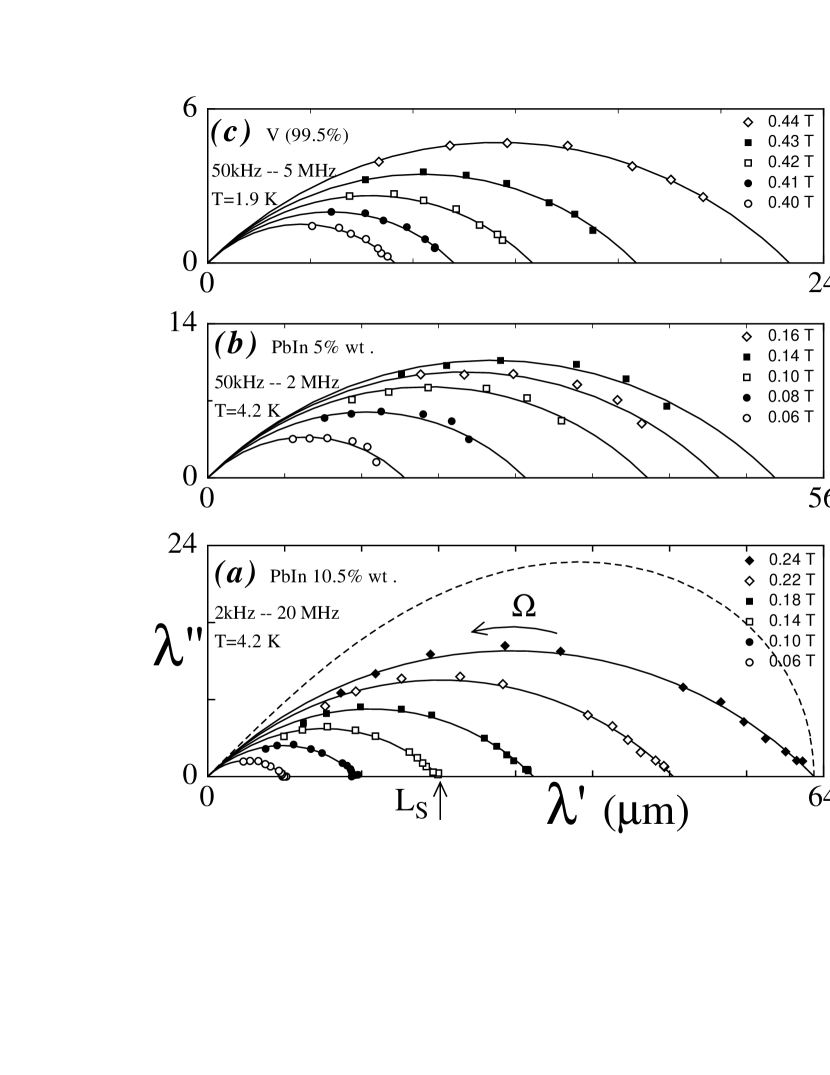
Figure 3: The apparent penetration depth $\lambda_{\rm ac}(\Omega)$ displayed in the complex plane. Data have been measured in the mixed state of conventional isotropic superconductors: Arc of circles (solid lines) are fitted to the data according to Eq. (14) by adjusting the skin length $L_{\rm S}$ (real-axis intercept indicated by an arrow in (a)). A typical bulk pinning spectrum, given by the Campbell expression (4) with $\lambda_{\rm C}=63\,\mu$m, has been plotted (dotted line) for comparison to the 0.24T data. (a) a $6(w)\times 4(t)\,$mm² slab of PbIn($10.5\%wt$) ($\rho_{\rm n}=10.3\,\mu\Omega$.cm); (b) a $5.8(w)\times 2(t)\,$mm² slab of PbIn($5\%wt$) ($\rho_{\rm n}=6.5\,\mu\Omega$.cm); (c) a $6.7(w)\times 1(t)\,$mm² vanadium slab ($\rho_{\rm n}=0.6\,\mu\Omega$.cm), spark-cut from a cold-rolled commercial plate.

Using condition (13) together with equations (8), (9) and (11), we determine $\tilde{b}_{1}$ in (12), which gives the following expression for the effective penetration depth:

$$\frac{1}{\lambda_{\rm ac}}=\frac{1}{L_{\rm S}}+\frac{1-{\rm i}}{\delta_{\rm f}},\qquad\mbox{where}\qquad L_{\rm S}=l\frac{\omega}{\mu_{0}\varepsilon}$$ (14)

is a length directly related to the roughness length $l$, and therefore connected with the order of magnitude of critical currents by $K_{\rm C}\sim\omega a/\mu_{0}L_{\rm S}$.

The frequency dependence of $\lambda_{\rm ac}$ is governed by that of the flux-flow skin depth $\delta_{\rm f}\propto 1/\sqrt{\Omega}$. The right-hand side of Eq. (14) is a straight line in the complex plane, which, by inversion, gives a quarter-circle for the spectrum $\lambda_{\rm ac}(\Omega)$ (Fig. 3). Through the action of the boundary conditions, it turns out that, in the low-frequency limit, $\lambda_{\rm ac}\simeq\tilde{b}_{1}\lambda_{\rm f}\simeq L_{\rm S}$ is real and independent of $\Omega$. The length $L_{\rm S}$, as $\lambda^{\prime}(0)$, plays the role of the Campbell length. We stress however that, in contrast to $\lambda_{\rm C}$, $L_{\rm S}$ is not an actual penetration depth, but rather some fraction of a much longer depth $\delta_{\rm f}$.

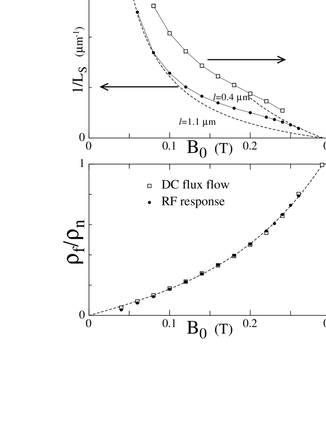
Figure 4: Upper panel : Typical field-dependences for the skin-length $L_{\rm S}$ (bullets) and the surface critical current density $K_{\rm C}$ (squares) in PbIn_10.5%w ($B_{\rm c2}=0.29\,$T, $\kappa\simeq 3.5$) at $T=4.2\,$K. Dotted lines are theoretical curves $L_{\rm S}=lB_{0}/\mu_{0}\varepsilon$ using the Abrikosov expression $\varepsilon\simeq(B_{\rm c2}-B_{0})/2.32\mu_{0}\kappa^{2}$, and a pinning length $l=1.1\,\mu$m (resp. $l=0.4\,\mu$m) for intermediate fields (resp. high fields). The product $K_{\rm C}L_{\rm S}\sim 10\,$mA agrees well with the theoretical estimate $\sqrt{B\varphi_{0}}/\mu_{0}$ ($=14$ mA at $B_{0}=0.15$ T) for surface pinning. Lower panel : the field dependence of the flux flow resistivity in PbIn${10.5\%w}$ at $T=4.2\,$K deduced from the slope of dc voltage-current characteristics (squares) and from rf surface impedance (bullets). rf data are deduced from the frequency dependence of $\lambda_{\rm ac}(\Omega)$ in Fig. 3a.

Fig. 2 shows a typical complex spectrum of $\lambda_{\rm ac}$ in a $\log$-frequency scale. Compared to our previous measurements [20], the number of frequency points and the frequency span have been doubled so as to cover most of the depinning transition. We confirm our observation that the cross-over is much broader than predicted by the Campbell bulk-pinning expression (4) (dotted lines in the figure) and extends over 6 decades of frequency ($10^{3}$–$10^{9}$ Hz in Fig.2). This observation is in apparent contradiction with that of Gittleman and Rosenblum [11] who reported a depinning transition in the ac resistivity of similar materials, over 2-decades of frequency. In fact, there is no inconsistency if one takes into account the finite thickness of their samples (see Sec. 5 below). The quality of the fit to Eq. (14) (solid line) in Fig.2 is, in itself, a strong indication for the two-mode electrodynamics. Apart from theoretical considerations, formula (14) proves powerful in extracting reliable values of the free-flow resistivity $\rho_{\rm f}$ within a few percent. This method compares favorably with microwave techniques.

The universal shape of the depinning spectra is well illustrated in the Argand diagram of Fig. 3, where data from two PbIn alloys ($\rho_{\rm n}=6.5$ and $10.3\,\mu\Omega$cm respectively)) and a vanadium sample ($\rho_{\rm n}=0.6\,\mu\Omega$cm) have been collected. The characteristic quarter-circle is observed in a variety of experimental conditions and samples, including very pure niobium ($\rho_{\rm n}\lesssim 10\,$n$\Omega$cm) in Ref. [20]. Two distinctive features, well observed in Fig. 3a, are worth mentioning : i) the linear behavior $\lambda^{\prime}\!+\!\lambda^{\prime\prime}\!=\!\lambda^{\prime}(0)$ at low frequency, and ii) the maximum of $\lambda^{\prime\prime}$, $\lambda^{\prime\prime}=\frac{1}{2}\tan(\pi/8)\lambda^{\prime}(0)=0.207\lambda^{\prime}(0)$, which is $30\%$ less than the generally accepted classical value $0.272\lambda^{\prime}(0)$.

The field dependence of both $L_{\rm S}$ and critical current densities $K_{\rm C}$ are shown in Fig. 4 (upper). The order of magnitude of the roughness length $l$ can be obtained by using the Abrikosov expression $\mu_{0}\varepsilon=(B_{\rm C2}\!-\!\omega)/2.32\kappa^{2}$ in $1/L_{\rm S}=\mu_{0}\varepsilon/l\omega$ and $\omega\!=\!B_{0}$. With $\kappa=3.5$ we find reasonable values $0.4<l<1\,\mu$m (dashed lines in Fig. 4). Moreover, $K_{\rm C}=I_{\rm C}/2w$ values, deduced from dc measurements, are also found to agree with the estimate $K_{\rm C}\approx\omega a/\mu_{0}L_{\rm S}$. Fig. 4 (lower) illustrates the resolution in $\rho_{\rm f}(\omega)$ achieved with rf surface impedance.

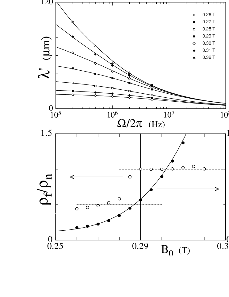
Figure 5: Upper panel: Continuity of the spectra $\lambda_{\rm ac}(\Omega)$ across the bulk-superconductivity transition in oblique field. Data are taken from a $6.1(w)\times 1.22(t)\,$mm² PbIn${10.5\%wt}$ at $T=4.2\,$K ($B_{\rm C2}=0.29\,$T). In this geometry, currents flow at 45 degrees to the magnetic field, and the penetration of the ac-field is symmetric over the four faces of the slab throughout the investigated range $0.9\leq B_{0}/B_{\rm C2}\leq 1.1$. Agreement with the theoretical spectrum (14) is observed on both sides of the transition which is a strong indication that the screening mechanism is the same in both cases. Lower panel : The skin-length $L_{\rm S}(B_{0})$ ($\bullet$) and the flux-flow resistivity $\rho_{\rm f}(B_{0})$ ($\circ$), deduced from the fits of $\lambda_{\rm ac}$. $L_{\rm S}(B_{0})$ is itself continuous through the transition, as is the dc critical current. The only accident observed at $B_{\rm C2}$ is a drop by a factor 2 in $\rho_{\rm f}(\pi/4)$ which signals the vanishing of the mixed-state anisotropy $\rho_{\rm f}(\theta)=\rho_{\rm f}(0)\cos^{2}\theta$.

4 Skin effect through the superconducting sheath

We have investigated the field range $B_{0}/B_{\rm C2}=$ 0.9–1.1 to explore the behaviour of the ac response in the transition from the bulk mixed state to the surface superconductivity. As surface superconductivity is not destroyed in oblique field, we took advantage of this geometry to symmetrize the role of the four faces of the sample (see Sec. 2). We recall that the superconducting sheath (depth $\sim\xi$) is populated by short vortices (flux spots) with a density $\omega=B_{0\perp}$ (see Ref. [22] and references therein).

The most striking fact in Fig. 5 is that, at the transition, there is no change in the shape of spectra, which, both above and below $B_{\rm C2}$, obey the theoretical expression (14). Above $B_{\rm C2}$ the bulk is normal, and the existence of screening surface currents is obvious; therefore, the two-mode electrodynamics and the free bulk penetration of the wave, which underlie Eq. (14), are not surprising.

Concerning the field-dependent parameters involved in Eq. (14), $L_{\rm S}$ and $\rho_{\rm f}$, we observe no discontinuity of $L_{\rm S}(B_{0})$, whereas a jump is observed in $\rho_{\rm f}$ as shown in Fig. 5b. The continuity of $L_{\rm S}(B_{0})$ is consistent with the observation that critical currents decrease monotonically through the transition together with the strength of the surface vortex state. The vanishing of the vortex structure in the bulk at $B_{\rm C2}$ results in an abrupt jump from $\rho_{\rm n}\cos^{2}\theta=\rho_{\rm n}/2$ to $\rho_{\rm n}$ as expected from the anisotropy of resistivity in the mixed state [22].

5 Size effects in thin slabs

Equation (14), and results in the above Section, concerned the ac response of two independent half spaces. In thin slabs and/or at low frequencies, fields penetrating from opposite faces interfere in the bulk whenever $t\lesssim 2\delta_{\rm f}$. Assuming symmetric surface conditions on both faces $z=\pm t/2$, the corresponding one-dimensional solution takes the even form :

$$\frac{b}{b_{0}}=\;\tilde{b}_{1}\frac{\cosh(z/\lambda_{\rm f})}{\cosh(t/2\lambda_{\rm f})} + \;\tilde{b}_{2}\frac{\cosh(z/\lambda_{\rm V})}{\cosh(t/2\lambda_{\rm V})}$$ (15)

$$\frac{E}{-i\Omega b_{0}}=\tilde{b}_{1}\lambda_{\rm f}\frac{\sinh(z/\lambda_{\rm f})}{\cosh(t/2\lambda_{\rm f})} + \tilde{b}_{2}\lambda_{\rm V}\frac{\sinh(z/\lambda_{\rm V})}{\cosh(t/2\lambda_{\rm V})}$$ (16)

$$\frac{B_{0}\nu}{b_{0}}=\;\tilde{b}_{1}\frac{\cosh(z/\lambda_{\rm f})}{\cosh(t/2\lambda_{\rm f})} - \frac{\omega}{\mu_{0}\varepsilon}\tilde{b}_{2}\frac{\cosh(z/\lambda_{\rm V})}{\cosh(t/2\lambda_{\rm V})}$$ (17)

$$\frac{B_{0}u}{b_{0}}=\tilde{b}_{1}\lambda_{\rm f}\frac{\sinh(z/\lambda_{\rm f})}{\cosh(t/2\lambda_{\rm f})} - \frac{\omega}{\mu_{0}\varepsilon}\tilde{b}_{2}\lambda_{\rm V}\frac{\sinh(z/\lambda_{\rm V})}{\cosh(t/2\lambda_{\rm V})}$$ (18)

The effective penetration depth reads

$$\lambda_{\rm ac}=\frac{E(t/2)-E(-t/2)}{-2{\rm i}\Omega b_{0}}=\tilde{b}_{1}\lambda_{\rm f}\;{\tanh(t/2\lambda_{\rm f})}+\tilde{b}_{2}\lambda_{\rm V}\simeq\tilde{b}_{1}\lambda_{\rm f}{\tanh(t/2\lambda_{\rm f})}.$$ (19)

Thin films ($t\lesssim 2\lambda_{\rm V}$) are excluded here by assuming ${\tanh(t/2\lambda_{\rm V})}=1$. Inserting boundary conditions $\nu(\pm t/2)=\mp u_{1}(\pm t/2)/l$, Eq. (14) becomes

$$\frac{1}{\lambda_{\rm ac}} = \frac{1}{L_{\rm S}}+\frac{1-i}{\delta_{\rm f}}\coth{\frac{(1-i)t}{2\delta_{\rm f}}}$$ (20)

$$\frac{1}{\lambda_{\rm ac}} \simeq \frac{1}{L_{\rm S}}+\frac{2}{t}\qquad\qquad(t/\delta_{\rm f}\rightarrow 0).$$ (21)

Comparing Eq. (20) with Eq. (14), it is seen that size effects will start when $t$ is decreased below about $3\delta_{\rm f}$, where the $\coth$ factor deviates significantly from unity. As a result losses are significantly reduced, the loss angle $\varphi$ falling off below the half-space level given by $\sin\varphi\!=\!|\lambda_{\rm ac}|/\delta_{\rm f}$. Data ($\varphi,|\lambda_{\rm ac}|$) obtained at 100 kHz in PbIn slabs, where $\rho_{\rm f}(B_{0})$ (then $\delta_{\rm f}$) had been separately measured, clearly demonstrate these size effects (see Fig.6). The fact that for decreasing sample thicknesses size effects are encountered when $t\sim\delta_{\rm f}$, i.e. well before $t\sim L_{\rm S}$, is not consistent with any one-mode theory (see Sec. 1).

According to Eq. (21), a second size effect occurs in the thin limit when $t\sim 2L_{\rm S}$. This second “dimensional” cross-over, which affects now the real part $\lambda^{\prime}$, could wrongly suggest that $L_{\rm S}$ is a true length in accordance with one-mode approaches. This shows that one must be careful in interpreting susceptibility measurements.

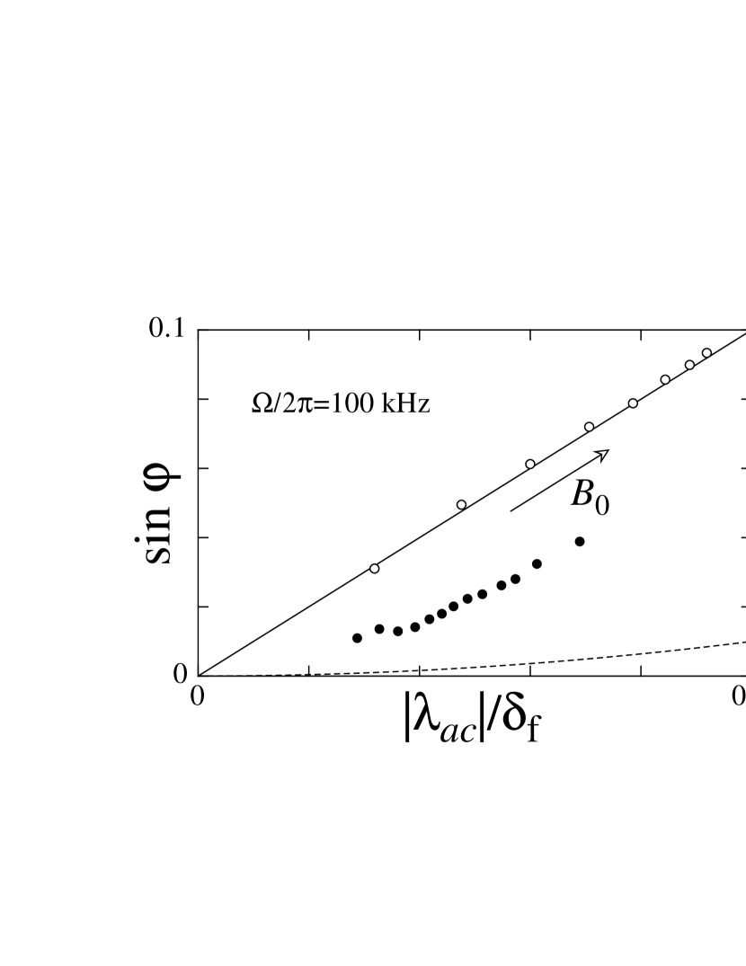
Figure 6: The sine of the loss-angle $\sin\varphi=\lambda^{\prime\prime}/|\lambda_{\rm ac}|$ as a function of $|\lambda_{\rm ac}|/\delta_{\rm f}$ in two slabs of the same PbIn${10.5\%wt}$ material with different thickness $t=0.3\,$mm ($\bullet$) and $t=1.3\,$mm ($\circ$). The skin-depth $\delta_{\rm f}$, or the flux-flow resistivity $\rho_{\rm f}$, is deduced from separate dc voltage-current characteristics. Data points ($|\lambda_{\rm ac}|,\varphi$) have been taken at a constant low frequency as a function of magnetic field : $B_{0}=0.04$–$0.18\,$T and $\delta_{\rm f}=0.13$–$0.32\,$mm in the $t=1.3\,$mm slab; $B_{0}=0.06$–$0.27\,$T and $\delta_{\rm f}=0.15$–$0.45\,$mm in the $t=0.3\,$mm slab. The theoretical law $\sin\varphi=|\lambda_{\rm ac}|/\delta_{\rm f}$ for the half space is well obeyed in the thick slab with $\delta_{\rm f}\lesssim t/4$, while a significant deficit in the losses of thin slab is observed for $\delta_{\rm f}\simeq 0.66$–$2t$. Note that, $|\lambda_{\rm ac}|\simeq 5$–$30\,\mu$m and $t=10$–$60|\lambda_{\rm ac}|$ in the same field range, so that no size effect would be expected if $\lambda_{\rm ac}$ was the actual penetration depth. Quantitative comparison with theory is difficult in this thin limit as losses become drastically sensitive to the symmetry of surface conditions (compare Eq. (19) with Eq. (23)).

Let us conclude by briefly examining resistivity measurements in foils within the thin limit. We refer in this respect to the pioneering work of Gittleman and Rosenblum [11], as also to recent measurements in YBaCuO platelets [23]. The analysis of such resistivity spectra is much more intricate. Many authors, using this method assume that the current density does not vary along the width $w$ of the foil; this requires the absence of two-dimensional skin-effects, $\delta_{\rm f}\gg w>t$, a condition that is hardly fulfilled over several frequency decades.

The one-dimensional treatment of the ac resistivity relies on the odd solution of Eqs. (6)–(9). The effective resistivity of the foil is defined as

$$\rho_{\rm ac}=\mu_{0}\frac{E(t/2)}{b_{0}}\;\frac{t}{2}=-{\rm i}\mu_{0}\Omega\lambda_{\rm ac}\;\frac{t}{2},$$ (22)

where

$$\frac{1}{\lambda_{\rm ac}}=\frac{1}{L_{\rm S}}+\frac{1-i}{\delta_{\rm f}}\tanh{\frac{(1-i)t}{2\delta_{\rm f}}}.$$ (23)

In the limit $t\ll 2\delta_{\rm f}$, Eqs. (22),(23) reduce to :

$$\frac{-{\rm i}\mu_{0}\Omega}{\rho_{\rm ac}}=\frac{2}{t\lambda_{\rm ac}}=\frac{2}{tL_{\rm S}}-\frac{2i}{\delta_{\rm f}^{2}}.$$ (24)

Surprisingly enough, we find the same resistivity spectrum as that given by Eq. (4) which follows from the bulk-pinning theory. Both Eqs. (4) and (24) equally fit the Gittleman-Rosenblum data (by setting $\lambda_{\rm C}=\sqrt{L_{\rm S}t/2}$ in Eq. (24)). We are led to the conclusion that resistivity experiments alone cannot decide between very contrasted models of pinning.

6 Conclusions

We have reported the first comprehensive investigation of dynamic depinning transition in the surface impedance geometry. It relies on the description of the depinning transition through Eq. (14) and requires the use of thick samples ($t\gtrsim 3\delta_{\rm f}$). The agreement is so good that surface-impedance measurements in the rf-domain provide a precise and accurate way of measuring both parameters $L_{\rm S}$ and $\rho_{\rm f}$. As shown in Fig. 4, dc data on the flux-flow resistivity, when available, confirm the accuracy of the method; in other cases where low-level ac techniques are necessary (large critical currents, ultra-low temperatures, …), the surface impedance becomes the best suited non-invasive method for measuring $\rho_{\rm f}$. Apart from this metrological aspect, it is clear that, as concerns the pinning length $L_{\rm S}=\lambda^{\prime}(0)$, our interpretation is completely at variance with classical views on pinning ([14] p. 345). In this respect we wish to add some comments.

The remarkable agreement with the two-mode spectrum (14) as well as the observation of predicted size effects for $t\sim\delta_{\rm f}$ at low frequencies bring out two important facts: i) The effective length, as deduced from the surface inductance $X/\Omega\!=\!\mu_{0}\lambda^{\prime}(0)$, is not an actual penetration depth; ii) free flow is observed in the bulk (over thicknesses $t\gtrsim 1$ mm), in spite of a large density of volume defects in a variety of polycrystalline samples from alloys to pure metals.

In the literature, $\lambda^{\prime}(0)$, usually referred to as the Campbell penetration depth, is directly expressed in terms of the bulk-pinning Labusch parameter $\alpha_{\rm L}$ (see Sec. 1). In soft samples, such as used in this work, bulk pinning is commonly analysed in the frame of the collective pinning theory of Larkin-Ovchinnikov [14], where $\alpha_{\rm L}$ is in turn related to Larkin transverse and longitudinal correlation lengths $R_{\rm C}$ and $L_{\rm C}$. These correlations lengths are intricate expressions of thermodynamic and pinning parameters (elastic constants $c_{44}$ and $c_{66}$, core radius $\xi$, pinning-centers concentration $n$ and the individual pinning force $f$). For thick samples (3D collective pinning) one expects that $\lambda^{\prime}(0)\approx L_{\rm C}\sim c_{44}c_{66}\xi^{2}/nf^{2}$ [13]. Thus many authors consider the lengths $\lambda^{\prime}(0)$ deduced from the low-frequency susceptibility as a routine measurement of $L_{\rm C}$ and merely investigate the field and temperature dependence of $L_{\rm C}$. This studies must be taken with due caution; our results show that a spectral analysis should precede any interpretation.

The role of point defects and elastic constants is certainly important in analyzing the short and long-range distortions of the vortex lattice, as observed in a number of techniques (Bitter decoration, neutron scattering, STM, …). However, our experiments seriously question the relevance of this mechanism of weak pinning in transport properties of soft samples. Here, we indeed exclude the case of hard materials where additional interfaces in the bulk may, to some extent, act like the surfaces of soft samples (twin planes in YBCO [24], precipitates in industrial wires, …).

The existence of a free vortex flow in the bulk, and the exclusive role of the surface in the critical-current properties of soft superconductors, have been confirmed in previous experiments under over-critical conditions: for instance the voltage and field noise in the flux-flow regime [25], the high-level step-response of a slab in parallel field [26], or surface localization of sub-critical currents [27], …We emphasize that these experiments have been specially designed to discriminate surface and bulk currents. It is clear that the existence of bulk sub-critical currents would imply bulk pinning, but there is up to now no experimental evidence for such bulk currents in soft samples. In particular one cannot, in this respect, rely on the recent Hall probe technique, which determines the radial distribution of the current in platelets. The observed pile-of-sand profile of the magnetic field confirms the critical state model [28], but critical state model should not be confused with bulk-pinning model. The critical-current densities in this geometry may be superficial and the technique used cannot resolve the axial distribution.

References

- [1] P. Mathieu, and Y. Simon, Europhys. Lett. 5, 67 (1988).
- [2] A.A. Abrikosov, M.P.Kemoklidze and I.M.Khalatnikov, Sov. Phys. JETP 21, 506 (1965).
- [3] T. Hocquet, P. Mathieu and Y. Simon, Phys. Rev. B 46, 1061 (1992).
- [4] I.L. Bekarevich and I.M. Khalatnikov, Sov. Phys. JETP 13, 643 (1961).
- [5] R.J. Donnelly, Quantized Vortices in Helium II, Cambridge University Press, Cambridge (1991).
- [6] T.D.C. Bevan, A.J. Manninen, J.B. Cook, H. Alles, J.R. Hook, and H.E. Hall, J. Low Temp. Phys. 109, 423 (1997).
- [7] C. Caroli, P.G. De Gennes and J. Matricon, Physics Letters 9, 307 (1964).
- [8] N.B. Kopnin and G.E. Volovik, Phys. Rev. Lett. 79, 1377 (1997).
- [9] B. Rosenblum and M. Cardona, Phys. Rev. Lett. 12, 657 (1964).
- [10] H. Vasseur, P. Mathieu, B. Plaçais and Y. Simon, Physica C 279, 103 (1997).
- [11] J.I. Gittleman and B. Rosenblum, Phys. Rev. Lett. 16, 734 (1966).
- [12] A.M. Campbell, J. Phys. C 2, 1492 (1969).
- [13] C.J. van der Beek, V.B. Geshkenbein and V.M. Vinokur, Phys. Rev. B 48, 3393 (1993).
- [14] M. Tinkham, Introduction to superconductivity, Second Edition (Mc Graw-Hill, 1996).
- [15] M.W. Coffey and J.R. Clem, Phys. Rev. Lett. 67, 386 (1991).
- [16] A.E. Koshelev and V.M. Vinokur, Physica C 173, 465 (1991).
- [17] E.B. Sonin, A.K. Tagantsev and K.B. Traito, Phys. Rev. B 46, 5830 (1992).
- [18] B. Plaçais, P. Mathieu, Y. Simon, E.B. Sonin and K.B. Traito, Phys. Rev. B 54, 13083 (1996).
- [19] P.G. De Gennes and J. Matricon, Review of Modern Physics 36, 45 (1964).
- [20] N. Lütke-Entrup, B. Plaçais, P. Mathieu and Y. Simon, Phys. Rev. Lett. 79, 2538 (1997).
- [21] D.E. Farrel, B.S. Chandrasekhar and H.V. Culpert, Phys. Rev. 177, 694 (1969).
- [22] P. Mathieu, B. Plaçais and Y. Simon, Phys. Rev. B 48, 7376 (1993).
- [23] H. Wu, N.P. Ong, R. Gagnon and L. Taillefer, Phys. Rev. Lett. 78, 334 (1997).
- [24] I. Maggio-Aprile, C. Renner, A. Erb, E. Walker and O. Fischer, Nature 390, 487 (1997).
- [25] B. Plaçais, P. Mathieu and Y. Simon, Phys. Rev. B 49, 15813 (1994).
- [26] H. Vasseur, P. Mathieu, B. Plaçais and Y. Simon, submitted to J. Phys. C.
- [27] P. Thorel, Y. Simon and A. Guetta, J. Low Temp. Phys. 11, 333 (1973).
- [28] Y. Abulafia, A. Shaulov, Y. Wolfus, R. Prozorov, L. Burlachkov, Y. Yeshurun, D. Majer, E. Zeldov and V.M. Vinokur, Phys. Rev. Lett. 75, 2404 (1995).