Ionic Reactions in Two Dimensions with Disorder

Abstract

We analyze the dynamics of the ion-dipole pairing reaction in the two-dimensional Coulomb gas in the presence of disorder. Sufficiently singular disorder forces the critical temperature of the Kosterlitz-Thouless-Berezinskii fixed point to be non-universal. This disorder leads to anomalous ion pairing kinetics with a continuously variable decay exponent. Sufficiently strong disorder eliminates the transition altogether. For ions that are chemically reactive, anomalous kinetics with a continuously variable decay exponent also occurs in the high-temperature regime. The Coulomb interaction inhibits reactant segregation, and so the ionic $\mbox{A}^{+}+\mbox{B}^{-}\to\emptyset$ reaction behaves like the nonionic $\mbox{A}+\mbox{A}\to\emptyset$ reaction.

]

I Introduction

The two-dimensional Coulomb gas has been the subject of careful attention since the elucidation of its low-temperature phase by Kosterlitz and Thouless [1] and Berezinskii [2]. Above a critical value of the dimensionless temperature, the system approximately obeys Debye-Hückle statistics (as it does for all temperatures in three dimensions). Below the transition temperature, ions of opposite charge pair to form dipoles. The temperature at which this metal-insulator transition occurs is universal in the absence of disorder. In the related superfluid system, this universality corresponds to the universal jump discontinuity in superfluid density (see [3] for a review).

The dynamics of the Coulomb gas under an external field has been analyzed by phenomenological extensions of the static Kosterlitz-Thouless argument [4, 5, 6, 7, 8, 9, 10, 11, 12, 13]. Different scaling regimes were found, and these are now understood to correspond to the cases of weak, slowly-varying or strong, rapidly-varying external fields [14]. While the equilibrium properties of the two-dimensional Coulomb gas have been established rigorously via field-theoretic analysis of the Sine-Gordon Hamiltonian [15, 16, 17, 18], there has been to date no rigorous, field-theoretic model for the ionic dynamics, near the low-temperature critical point or otherwise.

The dynamics of the two-dimensional reaction $\mbox{A}^{+}+\mbox{B}^{-}\to\emptyset$, where $\mbox{A}^{+}$ and $\mbox{B}^{-}$ are ions of opposite charge, has been studied in the high-temperature limit by scaling arguments and computer simulation. In the absence of Coulomb interaction, the A and B reactants segregate. This segregation leads to the diffusion-limited decay law $\langle c_{\rm A}(t)\rangle\sim[n_{0}/(8\pi^{2}Dt)]^{1/2}$ [19]. Local charge neutrality enforced by the Coulomb interaction inhibits this segregation of the reactants, allowing for a faster decay law. The charge density still decays as a power law, $\langle c_{\rm A}(t)\rangle\sim at^{-x}$. The decay exponent, $x$, has been observed in computer simulations to range from $0.79\pm 0.04$ [20] to $0.85\pm 0.05$ [21] to unity with logarithmic corrections [22]. Scaling theories have been proposed that lead to values for the decay exponent from $0.85$ [21, 23] to unity [24, 25]. An approximate, self-consistent treatment of the classical reaction diffusion equations leads to the prediction that the decay exponent is unity [26], although logarithmic corrections cannot be excluded due to the use of mean-field type equations.

Studies of single ion diffusion in correlated disorder have shown that for sufficiently long-ranged, disordered potential fields, anomalous diffusion occurs (see, for example, [11, 27, 28, 29, 30, 31, 32, 33, 34]). Ionic disorder in two dimensions creates just such a potential field, $v({\bf x})$, that leads to anomalous diffusion. As in previous work, we assume the potential to be Gaussian, with zero mean and correlation function $\chi_{vv}(r)$. The appropriate form for the Fourier transform at long wavelengths is $\hat{\chi}_{vv}({\bf k})=\int d{\bf x}\exp(i{\bf k}\cdot{\bf x})\chi_{vv}({\bf x})=\gamma/k^{2}$. This type of disorder leads to anomalous diffusion with a continuously variable exponent $\langle r^{2}(t)\rangle\sim bt^{1-\delta}$, where $\delta=1/[1+8\pi/(\beta^{2}\gamma)]$.

In this article, we use the rigorous field-theoretic formulation of reaction kinetics [35, 36, 37] to analyze both the ion-pairing reaction near the metal-insulator transition and the $\mbox{A}^{+}+\mbox{B}^{-}\to\emptyset$ annihilation reaction at high temperatures. The master equation description of this reaction is described in Section II. The field theory that we derive from this description is presented in Section III. Two dimensions is the upper critical dimension for this system—the dimension below which mean field theory fails. We derive the renormalization group flows for this system in Section IV. We give an asymptotically exact renormalization group analysis of the long-time dynamics in Section V. For the low temperature phase, we find a decay exponent that depends continuously on the strength of disorder. Moreover, we find that the critical temperature, which is universal in the absence of disorder, depends continuously on the strength of disorder. In Section VI we analyze the high-temperature dynamics of the $\mbox{A}^{+}+\mbox{B}^{-}\to\emptyset$ chemical reaction. We find a classical decay in the absence of disorder and anomalous kinetics in the presence of disorder. The Coulomb interaction prevents segregation of the reactants under all conditions, and so the dynamics of the ionic $\mbox{A}^{+}+\mbox{B}^{-}\to\emptyset$ reaction is similar to that of the neutral $\mbox{A}+\mbox{A}\to\emptyset$ reaction. We conclude in section VII with a discussion of the experimental implications of our results.

II Master Equation for Low-Temperature Ion Pairing

To analyze the ion pairing that takes place below the transition temperature, we consider the following reaction

$$\mbox{A}^{+}+\mbox{B}^{-}~{}{\mathrel{\mathop{\rightleftharpoons}\limits^{\lambda}_{\tau}}}~{}\mbox{C}\ ,$$ (1)

where $\mbox{A}^{+}$ and $\mbox{B}^{-}$ are the ions of opposite charge, and C is the dipole. We choose initially to have equal densities of ions $\langle c_{\rm A}(0)\rangle=\langle c_{\rm B}(0)\rangle=n_{0}$ and no dipoles. The ions are initially distributed at random, with Poissonian statistics. The long-time decay is not sensitive to short-ranged correlations that might be present in the initial conditions, such as those resulting from a high-temperature quench. The ion-dipole interaction will prove to be irrelevant, and so we can ignore the dipole orientation. The presence of the dipoles will, however, be relevant, and so it is necessary to include the reaction (1).

By considering the reaction on a lattice, we can write a master equation that governs changes in the densities of $\mbox{A}^{+}$, $\mbox{B}^{-}$, and C. The master equation relates how the probability, $P$, of a given configuration of particles on the lattice changes with time:

$$\frac{\partial P(\{m_{i}\},\{n_{i}\},\{l_{i}\},t)}{\partial t}=$$ (2)

$$\frac{D_{\rm A}}{(\Delta r)^{2}}\sum_{i,j}[T_{ji}^{\rm A}(m_{j}+1)P(m_{i}-1,m_{j}+1,t)$$ (3)

$$~{}~{}~{}~{}~{}~{}~{}~{}~{}~{}-T_{ij}^{\rm A}m_{i}P]$$ (4)

$$+\frac{D_{\rm B}}{(\Delta r)^{2}}\sum_{i,j}[T_{ji}^{\rm B}(n_{j}+1)P(n_{i}-1,n_{j}+1,t)$$ (5)

$$~{}~{}~{}~{}~{}~{}~{}~{}~{}~{}-T_{ij}^{\rm B}n_{i}P]$$ (6)

$$+\frac{D_{\rm C}}{(\Delta r)^{2}}\sum_{i,j}[(l_{j}+1)P(l_{i}-1,l_{j}+1,t)-l_{i}P]$$ (7)

$$+\frac{\lambda}{(\Delta r)^{2}}\sum_{i}[(m_{i}+1)(n_{i}+1)P(m_{i}+1,n_{i}+1,l_{i}-1,t)$$ (8)

$$~{}~{}~{}~{}~{}~{}~{}~{}~{}~{}-m_{i}n_{i}P]$$ (9)

$$+\tau\sum_{i}[(l_{i}+1)P(m_{i}-1,n_{i}-1,l_{i}+1,t)-l_{i}P]$$ (10)

Here $m_{i}$ is the number of A ions on site $i$, $n_{i}$ is the number of B ions on site $i$, and $l_{i}$ is the number of C particles at site $i$. The summation over $i$ is over all sites on the lattice, and the summation over $j$ is over the nearest neighbors of site $i$. The lattice spacing is given by $\Delta r$. The diffusive transition matrix for hopping from site $i$ to a nearest neighbor site $j$ is given by $T_{ij}^{\rm A}=[1+\beta(u_{i}^{\rm A}-u_{j}^{\rm A})/2]$ and $T_{ij}^{\rm B}=[1+\beta(u_{i}^{\rm B}-u_{j}^{\rm B})/2]$. Here $u$ is the sum of an external, quenched potential and the Coulomb potential created by all of the other ions. Specifically, $u_{i}^{\rm A}=v_{i}+\sum_{k}[m_{i+k}-\delta_{k0}-n_{i+k}]c_{k}$ and $u_{i}^{\rm B}=-v_{i}+\sum_{k}[n_{i+k}-\delta_{k0}-m_{i+k}]c_{k}$. Here $v_{i}$ is the external potential at site $i$, and $c_{k}$ is the Coulomb interaction $c({\bf r})=-J\ln(r)/(2\pi)$. For simplicity we will assume that the ions have the same diffusivity, $D_{\rm A}=D_{\rm B}=D$. The inverse temperature is given by $\beta=1/(k_{\rm B}T)$.

III The Field Theory

Using the coherent state representation, we map the master equation onto a field theory [35, 36, 37]. We incorporate a random potential into the field theory via the replica trick [19, 27]. We must also incorporate the ionic interaction into the field theory, taking care with self interaction terms.

The field theory that we generate is quadratic in the fields associated with the dipole density. Integrating out these fields, we are left with the action $S=S_{0}+S_{1}+S_{2}+S_{3}+S_{4}+S_{5}$

$$S_{0} = \int d^{d}{\bf x}\int_{0}^{t_{f}}dt\,\bar{a}_{\alpha}({\bf x},t)\left[\partial_{t}-D\nabla^{2}+\delta(t)\right]a_{\alpha}({\bf x},t)$$ (12)

$$+\int d^{d}{\bf x}\int_{0}^{t_{f}}dt\,\bar{b}_{\alpha}({\bf x},t)\left[\partial_{t}-D\nabla^{2}+\delta(t)\right]b_{\alpha}({\bf x},t)$$

$$S_{1} = -n_{0}\int d^{d}{\bf x}\left[\bar{a}_{\alpha}({\bf x},0)+\bar{b}_{\alpha}({\bf x},0)\right]$$ (13)

$$S_{2} = \lambda\int d^{d}{\bf x}\int_{0}^{t_{f}}dt\left[\bar{a}_{\alpha}({\bf x},t)\bar{b}_{\alpha}({\bf x},t)+\bar{a}_{\alpha}({\bf x},t)+\bar{b}_{\alpha}({\bf x},t)\right]$$ (15)

$$\times a_{\alpha}({\bf x},t)b_{\alpha}({\bf x},t)$$

$$S_{3} = -\lambda\tau\int d^{d}{\bf x}d^{d}{\bf x}^{\prime}\int_{0}^{t_{f}}dtdt^{\prime}$$ (18)

$$\times\left[\bar{a}_{\alpha}({\bf x},t)\bar{b}_{\alpha}({\bf x},t)+\bar{a}_{\alpha}({\bf x},t)+\bar{b}_{\alpha}({\bf x},t)\right]$$

$$\times G\!\!\!\!/({\bf x},{\bf x}^{\prime}|t,t^{\prime})a_{\alpha}({\bf x}^{\prime},t^{\prime})b_{\alpha}({\bf x}^{\prime},t^{\prime})$$

$$S_{4} = \beta J\int_{0}^{t_{f}}dt\int_{{\bf k}_{1}{\bf k}_{2}{\bf k}_{3}{\bf k}_{4}}$$ (23)

$$\times(2\pi)^{d}\delta({\bf k}_{1}+{\bf k}_{2}+{\bf k}_{3}+{\bf k}_{4})$$

$$\times\left[\hat{\bar{a}}_{\alpha}({\bf k}_{1},t)\hat{a}_{\alpha}({\bf k}_{2},t)-\hat{\bar{b}}_{\alpha}({\bf k}_{1},t)\hat{b}_{\alpha}({\bf k}_{2},t)\right]$$

$$\times\left[\hat{\bar{a}}_{\alpha}({\bf k}_{3},t)\hat{a}_{\alpha}({\bf k}_{4},t)-\hat{\bar{b}}_{\alpha}({\bf k}_{3},t)\hat{b}_{\alpha}({\bf k}_{4},t)\right]$$

$$\times\frac{{\bf k}_{1}\cdot({\bf k}_{1}+{\bf k}_{2})}{|{\bf k}_{1}+{\bf k}_{2}|^{2}}$$

$$S_{5} = \frac{\beta^{2}D^{2}}{2}\int_{0}^{t_{f}}dt_{1}dt_{2}\int_{{\bf k}_{1}{\bf k}_{2}{\bf k}_{3}{\bf k}_{4}}$$ (28)

$$\times(2\pi)^{d}\delta({\bf k}_{1}+{\bf k}_{2}+{\bf k}_{3}+{\bf k}_{4})$$

$$\times\left[\hat{\bar{a}}_{\alpha_{1}}({\bf k}_{1},t_{1})\hat{a}_{\alpha_{1}}({\bf k}_{2},t_{1})-\hat{\bar{b}}_{\alpha_{2}}({\bf k}_{1},t_{1})\hat{b}_{\alpha_{2}}({\bf k}_{2},t_{1})\right]$$

$$\times\left[\hat{\bar{a}}_{\alpha_{3}}({\bf k}_{3},t_{2})\hat{a}_{\alpha_{3}}({\bf k}_{4},t_{2})-\hat{\bar{b}}_{\alpha_{4}}({\bf k}_{3},t_{2})\hat{b}_{\alpha_{4}}({\bf k}_{4},t_{2})\right]$$

$$\times{\bf k}_{1}\cdot({\bf k}_{1}+{\bf k}_{2}){\bf k}_{3}\cdot({\bf k}_{1}+{\bf k}_{2})\hat{\chi}_{vv}(|{\bf k}_{1}+{\bf k}_{2}|)\ .$$

Summation is implied over replica indices. The notation $\int_{\bf k}$ stands for $\int d^{d}{\bf k}/(2\pi)^{d}$. The upper time limit in the action is arbitrary as long as it exceeds times for which we wish to make calculations. The random, Poissonian initial condition is accounted for by the term $S_{1}$. The forward reaction is captured by the term $S_{2}$. The effective potential due to the dipoles is captured by the term $S_{3}$. The propagator of the dipoles is given by

$$\hat{G\!\!\!\!/}(k,t)=\left\{\begin{array}[]{l}\exp[-(D_{\rm C}k^{2}+\tau)t],~{}t>0\\[14.45377pt] 0,t\leq 0\end{array}\right.\ ,$$ (29)

where $D_{\rm C}$ is the diffusion coefficient of the dipoles. At long times, the ion density will be much smaller than the dipole density, and we can replace the instantaneous dipole density with the average density. This simplifies the effective dipole term to

$$S_{3}^{\prime} = -n_{\rm c}\tau\int d^{d}{\bf x}\int_{0}^{t_{f}}dt$$ (31)

$$\times\left[\bar{a}_{\alpha}({\bf x},t)\bar{b}_{\alpha}({\bf x},t)+\bar{a}_{\alpha}({\bf x},t)+\bar{b}_{\alpha}({\bf x},t)\right]\ ,$$

with $n_{\rm c}=n_{0}-\langle c_{\rm A}(t)\rangle\sim n_{0}$. This modified action is identical to that for the reaction

$$\mbox{A}^{+}+\mbox{B}^{-}~{}{\mathrel{\mathop{\rightleftharpoons}\limits^{\lambda}_{n_{\rm c}\tau}}}~{}\emptyset\ .$$ (32)

This reaction can be recognized as the one addressed by the usual Sine-Gordon model of the Coulomb gas, with the equilibrium ionic density, $y$, given at low densities by $y^{2}=n_{\rm c}\tau/\lambda$. The flow equations for these two forms, $S_{3}$ and $S_{3}^{\prime}$, are, of course, equivalent. The Coulomb interaction between the ions is captured by the term $S_{4}$. Note that the Coulomb coupling should be an effective one, including a finite renormalization due to dipole screening. The effective potential due to the randomness is captured in the term $S_{5}$.

The concentrations, averaged over initial conditions, are given by

$$\langle c_{\rm A}({\bf x},t)\rangle = \lim_{N\to 0}\langle a({\bf x},t)\rangle\$$ (33)

$$\langle c_{\rm B}({\bf x},t)\rangle = \lim_{N\to 0}\langle b({\bf x},t)\rangle\ \ ,$$ (34)

where the average on the right hand side is taken with respect to $\exp(-S)$.

IV Renormalization Group Flows

We use renormalization group theory to deduce the long-time scaling of the ionic concentration. The diagrams that we need to consider are illustrated in Figure 1.

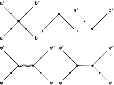
FIG. 1.: The vertices considered in the field theory. We have set $a^{*}=\bar{a}+1$ and $b^{*}=\bar{b}+1$. All combinations of $\varphi=a,b$ and $\psi=a,b$ are considered.

The one-loop flow equations that result are

$$\frac{d\ln n_{\rm c}}{dl} = 2$$ (35)

$$\frac{d\ln\lambda}{dl} = -\frac{\lambda}{4\pi D}+\frac{\beta J}{2\pi}-\frac{\beta^{2}\gamma}{4\pi}$$ (36)

$$\frac{d\ln\left(n_{\rm c}\tau/\lambda\right)}{dl} = 4-\frac{\beta J}{2\pi}+\frac{\beta^{2}\gamma}{2\pi}$$ (37)

$$\frac{d\ln(\beta J)}{dl} = -\frac{\lambda^{2}\beta J}{2\pi D^{2}}\frac{n_{\rm c}\tau}{\lambda\Lambda^{4}}$$ (38)

$$\frac{d\ln(\beta^{2}\gamma)}{dl} = -\frac{\lambda^{2}\beta J}{\pi D^{2}}\frac{n_{\rm c}\tau}{\lambda\Lambda^{4}}\ ,$$ (39)

where $\Lambda$ is the cutoff in Fourier space. The dynamical exponent is given by

$$z=2+\frac{\beta^{2}\gamma}{4\pi}+\frac{\beta^{2}\gamma}{4\pi}\frac{\lambda^{2}}{D^{2}}\frac{n_{\rm c}\tau}{\lambda\Lambda^{4}}\ .$$ (40)

These flow equations are valid to first order in $\tau$. At this order, they are valid to all orders in $\beta J$. Also at this order, the flow equation for $\beta^{2}\gamma$ is likely valid to all orders in $\beta^{2}\gamma$ [19, 38]. The flow equation for $\lambda$ may contain contributions from higher orders in $\beta^{2}\gamma$.

V Matching and Results

To compute the long-time value of the ionic concentration, we integrate the flow equations up to a matching time, $t_{0}$. We match the results of the flow equations to a mean field theory that is valid for short times. At these short times, we need not worry about renormalization of the reaction rates or Coulomb coupling. Furthermore, the reaction dynamics occurs in a local region, where the random potential is roughly constant, and so we may assume normal diffusive behavior. In other words, we can use the standard, classical reaction diffusion equations. A self-consistent treatment of these equations has recently been presented [26]. This theory suggests that the Coulomb interaction prevents segregation of the reactants. Moreover, the reaction is not limited by local transport as long as $\lambda\leq 2\beta JD$. We see that this condition is satisfied by the fixed point forward rate, and so the concentration is given by

$$\langle c_{\rm A}(t(l),l)\rangle=1/\left[1/n_{0}(l)+\lambda^{*}t(l)\right]\ .$$ (41)

We find the physical concentration from the relation

$$\langle c_{\rm A}(t)\rangle=e^{-2l}\langle c_{\rm A}(t(l),l)\rangle\ .$$ (42)

The result is

$$\langle c_{\rm A}(t)\rangle\sim\frac{1}{\lambda^{*}t}\left(\frac{t}{t_{0}}\right)^{\delta}\ ,$$ (43)

with the fixed point reaction rate given from Eq. (39) as $\lambda^{*}/D=2\beta J^{*}-\beta^{2}\gamma^{*}=16\pi+\beta^{2}\gamma^{*}$. Interestingly, we see that $\lambda^{*}$ is finite at the Kosterlitz-Thouless fixed point, where $(n_{\rm c}\tau)^{*}$ vanishes. Dipole dissociation, then, is key to the physics of the low-temperature fixed point.

We see that the ions pair according to the classical law in the absence of disorder. In the presence of disorder, we find anomalous kinetics. The kinetics is anomalous because at long-times and low concentrations the reaction becomes diffusion limited, and at long times the diffusion is anomalous in the type of disorder that we are considering. Note that this result for the ion pairing in disorder below the transition temperature is identical to that for the $\mbox{A}+\mbox{A}\to\emptyset$ reaction with disorder [38], except for a different value of $\lambda^{*}$.

If we interpret these flow equations as relations between related equilibrium models, we recognize the standard Kosterlitz-Thouless result when disorder is absent, with $y^{2}=\langle c_{\rm A}\rangle^{2}=n_{\rm c}\tau/\lambda$. Figure 2 shows the flows for the case of weak disorder.

FIG. 2.: The flow of the equilibrium ion density near the low-temperature critical point. Below the critical temperature the ion density is driven to zero as dipoles are formed. Above the critical temperature the dipoles unpair, and the ion density becomes large. For each curve, $\beta^{2}\gamma=1$ and $\lambda/D=16\pi+1$ at the point closest to the critical point.

Interestingly, we can deduce the one-loop critical temperature in the presence of disorder with an extension of the elementary Kosterlitz-Thouless free energy argument [1]. This argument predicts that the ion pairs will unbind when the free energy to create two unbound ions, $F_{\pm}=(E_{+}+E_{-})-T(S_{+}+S_{-})$, is positive. The Coulomb energy of the ion pair is, of course, $U_{\rm C}(r)=J\ln(r)/(2\pi)$. The effective interaction between an ion pair due to the random potential is given by $U_{\rm Veff}(r)=-\beta^{-1}\ln\langle\exp\{-\beta[v(0)-v(r)]\}\rangle=-\beta\gamma\ln(r)/(2\pi)$. Quenched and annealed statistics are identical here for an ion pair seperated by a finte distance, $r$, in a sufficiently large disordered medium, since the correlations in the potential for the ion pair are short ranged [39, 40]. The entropy of the ion pair is, of course, $4k_{\rm B}\ln(r)$. The ions, therefore, proliferate when $\beta J-\beta^{2}\gamma<8\pi$. This condition is exactly the one contained in the flows of Eq. (39) near the low-temperature fixed point. This energy-entropy argument is not strictly rigorous, since the metal-insulator transition occurs for $r\approx L$, where $L$ is the system size. In this regime, the correlations in the potential for the ion pair are not short-ranged, and quenched and annealed statistics are not strictly equal. What we have shown is that to one loop order these distinct statistics lead to the same behavior. Unless something unexpected occurs in the regime $r\approx L$, our location of the critical point may be exact to all orders.

The transition temperature, which is universal in the absence of disorder, becomes continuously variable in the presence of disorder. This is a unique feature of the ionic disorder that we are considering. The system undergoes a transition from insulator to metal either by decreasing $\beta J$ or by increasing the density of defects, $\rho=\sqrt{\gamma}/J$. Figure 3 shows the phase diagram of the system at infinitesimally small total (free plus bound) ion density.

FIG. 3.: The Kosterlitz-Thouless-Berezinskii fixed line in the presence of disorder (solid) for infinitesimally small total ion density. Here $\rho=\sqrt{\gamma}/J$ is roughly the density of defects. The system is an insulator below the curve.

Note that sufficiently strong disorder eliminates the insulating phase completely. A similar type of equilibrium phase diagram has been predicted for two-dimensional crystals with random substitutional disorder [41, 42]. This substitutional disorder is equivalent, in our language, to random, quenched dipoles. So we see that quenched ions obeying bulk charge neutrality behave in the long-wavelength limit in the same way as random, quenched dipoles.

A reentrant metallic phase may occur at low temperatures. This insulating to conducting transition may occur because the forces arising from the disorder, which tend to separate the ion pairs, are a factor $1/T$ greater than the bare Coulomb forces. Figure 4 shows the reentrant phase diagram predicted by the flow equations for $\rho=\sqrt{\gamma}/J=0.05$ for a range of initial values of $y=\langle c_{\rm A}\rangle=[n_{\rm c}\tau/\lambda]^{1/2}$ and $\beta J$.

FIG. 4.: The Kosterlitz-Thouless-Berezinskii fixed line in the presence of a fixed amount of disorder, $\rho=\sqrt{\gamma}/J=0.05$. Note the reentrant phase at low temperatures for a finite density of free ions, $y$. The curve is strictly valid only in the high-temperature regime (solid).

The temperature at which the reentrant phase occurs is roughly proportional to $\sqrt{\gamma}$. Since our flow equations are an expansion in $\beta^{2}\gamma$, they are not strictly valid in the reentrant regime. Thus, the existence of the reentrant phase, while physically plausible, cannot be rigorously established with our flow equations. A similar reentrant phase diagram has been predicted for the equilibrium XY model with random Dzyaloshinskii-Moriya interactions, which leads again, in our language, to a two-dimensional Coulomb gas with random, quenched dipoles [43].

The ratio $\rho=\sqrt{\gamma}/J$ remains constant under renormalization. This means that we can define $\gamma=\gamma_{0}/\epsilon^{2}$ and $J=J_{0}/\epsilon$, and one flow equation for $\epsilon$ will result. This factor $\epsilon$ is none other than the dielectric constant! The disorder term contains two powers of the dielectric constant because it is a correlation function of the disorder potential. The flow equation for $\epsilon$ is not universal [15, 16, 17, 18] and should probably include additional (finite) terms.

VI High-Temperature Dynamics

We now turn to consider two-dimensional ionic reactions at high temperatures. That is, we consider the reaction

$$\mbox{A}^{+}+\mbox{B}^{-}~{}{\mathrel{\mathop{\to}\limits^{k}}}~{}\mbox{P}\ ,$$ (44)

where P is the neutral product of the reaction. In the high-temperature regime, the ions pair to an insignificant extent. This follows from physical considerations. This conclusion also follows from the flow equations that drive the ion density to large values. Since the dipole density is insignificant, we may ignore the ion-dipole reaction. By comparing Eq. (44) with Eq. (32), we see that the appropriate action for this reaction is Eq. (28) with the replacement $\lambda\to k$, $\tau\to 0$, and $n_{\rm c}\to n_{0}$. The flow equations for this case are

$$\frac{d\ln n_{0}}{dl} = 2$$ (45)

$$\frac{d\ln k}{dl} = -\frac{k}{4\pi D}+\frac{\beta J}{2\pi}-\frac{\beta^{2}\gamma}{4\pi}$$ (46)

$$\frac{d\ln(\beta J)}{dl} = 0$$ (47)

$$\frac{d\ln(\beta^{2}\gamma)}{dl} = 0\ .$$ (48)

In this case, $\beta J$ is a constant to all orders. As before [19, 38], it seems likely that $\beta^{2}\gamma$ is a constant to all orders. The flow equation for $k$ is accurate to first order only in $\beta^{2}\gamma$. For our purpose, we will assume that the fixed point reaction rate, $k^{*}/D=2\beta J-\beta^{2}\gamma$, is always positive. Note that irrelevant details can renormalize (a finite amount) all of the parameters of the model. Dipole screening leading to a dielectric constant greater than unity is an example of this phenomenon.

We can again perform the matching. Since at the fixed point the reaction step is still rate limiting [26], we find the same classical decay as for the ion-pairing reaction:

$$\langle c_{\rm A}(t)\rangle\sim\frac{1}{k^{*}t}\left(\frac{t}{t_{0}}\right)^{\delta}\ .$$ (49)

Since reactant segregation is suppressed, this result for the high-temperature ionic reaction $\mbox{A}^{+}+\mbox{B}^{-}\to\emptyset$ is identical to that for the neutral reaction $\mbox{A}+\mbox{A}\to\emptyset$ except for a different value of $k^{*}$ [38].

VII Conclusions

There are many systems well-modeled by the 2-D Coulomb gas. A simple physical system might be, for example, ions confined to a thin film between two insulators. Other examples include dislocations or disclinations in systems such as charge density waves, Abrikosov flux lattices, or Langmuir-Blodgett films. In all cases, the defects unbind at higher temperatures, in a form of Kosterlitz-Thouless-Berezinskii transition. In the case of disclinations, or scalar charges, this transition is exactly of the form that we consider, and the system is a perfect instance of the 2-D Coulomb gas model. The type of disorder that we consider often comes about in these systems via pinning of some of the defects. The density of impurities, which are disrupting the low-temperature phase, can be controlled via the number of surface defects and is given roughly by $\rho=\sqrt{\gamma}/J$.

For these systems we make the following experimental predictions. There should be a continuously-variable transition temperature in the presence of long-ranged, logarithmic-type disorder. This type of disorder is naturally induced by impurity phases in these systems. This equilibrium behavior has, in fact, been seen in the melting of hexatic monolayers [44] and hexatic charge density waves [45, 46], where disclinations pinned by surface defects lead to a continuous lowering of the hexatic-liquid transition temperature. In other words, these experiments have shown that the order-disorder transition can be driven either by increasing temperature or by increasing disorder. In terms of Figure 3, these experiments crossed the transition line by increasing the disorder, i. e. by moving vertically upwards. Ionic reactions, such as those considered in [20, 21, 22, 23, 24, 25, 26], should decay as $\langle c_{\rm A}(t)\rangle\sim 1/(2\beta JDt)$ at long times in the absence of disorder. In the presence of long-ranged, logarithmic-type disorder [11, 27, 28, 29, 30, 31, 32, 33, 34], ions at finite density should pair in the low-temperature phase according to Eq. (43). Finally, the concentration of ions undergoing a bimolecular chemical reaction at high temperature in this same type of disorder should decay as Eq. (49).

REFERENCES

- [1] J. M. Kosterlitz and D. J. Thouless, J. Phys. C 6, 1181 (1973).
- [2] V. L. Berezinskii, Z. Eksp. Teor. Fiz 61, 1144 (1971), [Sov. Phys.-JETP 34, 610 (1971)].
- [3] D. R. Nelson, in Phase Transitions and Critical Phenomena, edited by C. Domb and J. Lebowitz (Academic Press, New York, 1983), Vol. 7.
- [4] J. L. McCauley, J. Phys. Chem. 10, 689 (1977).
- [5] B. A. Huberman, R. J. Myerson, and S. Doniach, Phys. Rev. Lett. 40, 780 (1978).
- [6] R. J. Myerson, Phys. Rev. B 18, 3204 (1978).
- [7] V. Ambegaokar, B. I. Halperin, D. R. Nelson, and E. D. Siggia, Phys. Rev. Lett. 40, 783 (1978).
- [8] V. Ambegaokar, B. I. Halperin, D. R. Nelson, and E. D. Siggia, Phys. Rev. B 21, 1806 (1980).
- [9] B. I. Halperin and D. R. Nelson, J. Low Temp. Phys. 36, 599 (1979).
- [10] V. Ambegaokar and S. Teitel, Phys. Rev. B 19, 1667 (1979).
- [11] D. S. Fisher, M. P. A. Fisher, and D. A. Huse, Phys. Rev. B 43, 130 (1991).
- [12] A. Dorsey, Phys. Rev. B 43, 7575 (1991).
- [13] P. Minnhagen, O. Westman, A. Jonsson, and P. Olsson, Phys. Rev. Lett. 74, 3672 (1995).
- [14] D. Bormann, Phys. Rev. Lett. 78, 4324 (1997).
- [15] T. Ohta, Prog. Theo. Phys. 60, 968 (1978).
- [16] T. Ohta and D. Jasnow, Phys. Rev. B 20, 139 (1979).
- [17] H. J. F. Knops and L. W. J. den Ouden, Physica A 103, 597 (1980).
- [18] D. J. Amit, Y. Y. Goldschmidt, and G. Grinstein, J. Phys. A 13, 585 (1980).
- [19] M. W. Deem and J.-M. Park, Phys. Rev. E 57, 2681 (1998).
- [20] G. Huber and P. Alstrom, Physica A 195, 448 (1993).
- [21] W. G. Jang, V. V. Ginzburg, C. D. Muzny, and N. A. Clark, Phys. Rev. E 51, 411 (1995).
- [22] B. Yurke, A. N. Pargellis, T. Kovacs, and D. A. Huse, Phys. Rev. E 47, 1525 (1993).
- [23] V. V. Ginzburg, P. D. Beale, and N. A. Clark, Phys. Rev. E 52, 2583 (1995).
- [24] G. S. Oshanin, A. A. Ovchinnikov, and S. F. Burlatsky, J. Phys. A 22, L977 (1989).
- [25] I. Ispolatov and P. Krapivsky, Phys. Rev. E 53, 3154 (1996).
- [26] V. V. Ginzburg, L. Radzihovsky, and N. A. Clark, Phys. Rev. E 55, 395 (1997).
- [27] V. E. Kravtsov, I. V. Lerner, and V. I. Yudson, J. Phys. A 18, L703 (1985).
- [28] V. E. Kravtsov, I. V. Lerner, and V. I. Yudson, Phys. Lett. A 119, 203 (1986).
- [29] J. P. Bouchaud, A. Comtet, A. Georges, and P. L. Doussal, J. Phys 48, 1445 (1987).
- [30] J. P. Bouchaud, A. Comtet, A. Georges, and P. L. Doussal, J. Phys 49, 369 (1988).
- [31] J. Honkonen, Y. M. Pis’mak, and A. V. Vasil’ev, J. Phys. A 21, L835 (1988).
- [32] J. Honkonen and Y. M. Pis’mak, J. Phys. A 22, L899 (1989).
- [33] S. É. Derkachov, J. Honkonen, and Y. M. Pis’mak, J. Phys. A 23, L735 (1990).
- [34] S. É. Derkachov, J. Honkonen, and Y. M. Pis’mak, J. Phys. A 23, 5563 (1990).
- [35] L. Peliti, J. Phys. A 19, L365 (1986).
- [36] B. P. Lee, J. Phys. A 27, 2633 (1994).
- [37] B. P. Lee and J. Cardy, J. Stat. Phys. 80, 971 (1995); 87, 951 (1997).
- [38] J.-M. Park and M. W. Deem, Phys. Rev. E 57, 3618 (1998).
- [39] M. E. Cates and R. C. Ball, J. Phys. (Paris) 49, 2009 (1988).
- [40] D. Wu, K. Hui, and D. Chandler, J. Chem. Phys. 96, 835 (1992).
- [41] D. R. Nelson, Phys. Rev. B 27, 2902 (1983).
- [42] M.-C. Cha and H. A. Fertig, Phys. Rev. Lett. 74, 4867 (1995).
- [43] M. Rubinstein, B. Shraiman, and D. R. Nelson, Phys. Rev. B 27, 1800 (1983).
- [44] R. Viswanathan, L. L. Madsen, J. A. Zasadzinski, and D. K. Schwartz, Science 269, 51 (1995).
- [45] H. J. Dai and C. M. Lieber, Phys. Rev. Lett. 69, 1576 (1992).
- [46] H. J. Dai, J. Liu, and C. M. Lieber, Phys. Rev. Lett. 72, 748 (1994).