PHYSICAL REVIEW B     VOLUME 57, NUMBER 21 1 JUNE 1998-I, 13639$-$13654 Quantum-classical transition of the escape rate of a uniaxial spin system
in an arbitrarily directed field

I Introduction

The two fundamental mechanisms of the escape of a particle from a metastable potential well are quantum tunneling through the barrier and the classical thermal activation over the barrier. The first mechanism is closely related to the tunneling level splitting for a particle in a double-well potential, which was considered by Hund [5] for the ammonia molecule. Other early studies based on the WKB approximation [6, 7, 8] treated the ionization of atoms in electric fields, [9] cold emission of electrons from metal surfaces, [10] and decay of nuclei. [11] Tunneling in spin systems was considered much later: Korenblit and Shender [12] calculated the ground-state splitting in the high-spin rare-earth compounds with the help of a high-order perturbation theory, Chudnovsky [13] applied the instanton technique for the Landau-Lifshitz equation to calculate the escape rates. The current broad interest to the spin-tunneling problem was initiated, however, mainly by the application of the instanton method by Enz and Schilling [14] and Chudnovsky and Gunther, [15] and the spin-WKB formalism by van Hemmen and Sütő. [16]

Studying thermally activated escape of a classical particle from the metastable minimum of a potential $U(x)$ goes back to Kramers, [17] who solved the Fokker-Planck equation describing the diffusion of the particle over the barrier. For spin systems, the role of thermal agitation in overcoming energy barriers (described, e.g., by the Stoner-Wohlfart model [18]) was stressed by Néel. [19] Brown [20] has derived the Fokker-Planck equation for classical spin systems and calculated the escape rate in the uniaxial model.

An extensive reference to the thermal activation and tunneling of particles can be found in Ref. [21], to magnetization tunneling in Ref. [22], and to the thermal activation in classical spin systems in Ref. [23]. Spin tunneling was recently observed in small magnetic particles such as ferritin [24, 25, 26] and barium ferrite, [27] and in high-spin molecules, Mn₁₂Ac [28, 29, 30, 31, 32] (see also Refs.  [33]) and Fe₈. [34]

Considering escape at finite temperatures, the first idea is to sum the tunneling and thermoactivation escape rates as stemming from independent channels: $\Gamma=\Gamma_{q}+\Gamma_{\rm th}$. Since the thermoactivation rate follows the very steep Arrhenius temperature dependence, $\Gamma_{\rm th}=\Gamma_{0}\exp(-\Delta U/T)$, the transition between quantum and classical regimes occurs at the temperature $T_{0}$ defined by $\Gamma_{q}=\Gamma_{\rm th}(T_{0})$. Writing $\Gamma_{q}=A\exp(-B)$, ignoring prefactors and equating the exponents, one obtains the estimation

$$T_{0}^{(0)}=\Delta U/B,$$ (1)

where the superscript at $T_{0}$ says that the ground-state tunneling is considered. For $T>T_{0}^{(0)}$ one has practically $\Gamma\cong\Gamma_{\rm th}(T)$, whereas below the transition $\Gamma\cong\Gamma_{q}$ is independent of temperature. The transition between the two regimes occures on the temperature interval $\Delta T\sim T_{0}^{(0)}/B$. Since $B\propto S$, this is much smaller than $T_{0}^{(0)}$ in the quasiclassical limit, $S\gg 1$. The simple scenario above is the prototype for the so-called first-order quantum-classical transition of the escape rate, which is accompanied by the discontinuity of $d\Gamma/dT$ at $T_{0}$.

It turns out, however, that for common metastable or double-well potentials, such as cubic or quartic parabola, another scenario is realized. Below the crossover temperature $T_{0}$ the particles cross the barrier at the most favorable energy level $E(T)$ which goes down from the top of the barrier to the bottom of $U(x)$ with lowering temperature. Such a regime is called thermally assisted tunneling (TAT). The transition from the classical regime to TAT is smooth, with no discontinuity of $d\Gamma/dT$ at $T_{0}$, and the transition temperature is given by [35]

$$T_{0}^{(2)}=\tilde{\omega}_{0}/(2\pi),\qquad\tilde{\omega}_{0}=\sqrt{|U^{\prime\prime}(x_{\rm sad})|/m}.$$ (2)

Here the superscript in $T_{0}$ denotes the second-order transition, $x_{\rm sad}$ corresponds to the top of the barrier (the saddle point of the potential), and $\tilde{\omega}_{0}$ is the so-called instanton frequency. In fact, the above formula is valid in the moderate-damping case, in which the Kramers’ result for the classical escape rate is independent of the friction constant $\eta$ and coincides with that of the simple transition-state theory (TST). In the strong- and weak-damping cases $\Gamma_{0}\propto 1/\eta$ and $\Gamma_{0}\propto\eta$, respectively, [17] and the formula (2) should be modified (see, e.g., Ref. [21]). The consideration in the moderate-damping case is the most simple, and all the results can be obtained from the simple quantum TST formula neglecting dissipation and giving the escape rate as a Boltzmann average of quantum escape rates at different energies. [36, 37] The quantum-classical transition of the escape rate including the dissipation in the strong- to moderate-damping regimes was described with the help of the Caldeira-Leggett formalism [38] in Refs.  [39, 40, 41, 42, 43]. The results show that in the exponential approximation for the escape rate only the second derivative $d^{2}\Gamma/dT^{2}$ is discontinuous at $T_{0}^{(2)}$. More accurate calculations taking into account the prefactor [37, 40] show the smoothening of the transition in the vicinity of $T_{0}^{(2)}$ due to quantum effects and the thermal distribution, so that all the derivatives of $\Gamma(T)$ behave continuously.

The terms first- and second-order quantum-classical transitions of the escape rate used above are due to Larkin and Ovchinnikov. [44] Chudnovsky [45] stressed the analogy with the phase transitions and analyzed the general conditions for both types of quantum-classical transitions. He has shown that for the second-order transition the period of oscillations $\tau(E)$ in the inverted potential $-U(x)$ should monotonically increase with the amplitude of oscillations, i.e., with the lowering energy $E$ from the top of the barrier. If $\tau(E)$ is nonmonotonic, the first-order transition occurs. Quite recently an effective free energy $F(E)$ for quantum-classical transitions of the escape rate of a spin system was written, [46] the minimization of which determines the escape rate in the exponential approximation: $\Gamma\sim\exp(-F_{\rm min}/T)$. The latter has the form $F=a\phi^{2}+b\phi^{4}+c\phi^{6}+F_{0}$, just as in the Landau model of phase transitions. [47] Here $a=0$ corresponds to the quantum-classical transition and $b=0$ to the boundary between first- and second-order transitions.

In a sense, second-order quantum-classical transitions of the escape rate are common, whereas the first-order ones are exotic and have to be specially looked for. Nevertheless, a number of systems and processes showing first-order transitions are already known, e.g., a SQUID with two Josephson junctions, [48] false vacuum decay in field theories, [49, 50, 51, 52] and depinning of a massive string from a linear defect. [53, 54] All these systems have more degrees of freedom than just a particle, thus the search for a physical system equivalent to a particle in a potential $U(x)$ leading to the first-order transition of the escape rate seems to be quite actual. Qualitatively it is clear how $U(x)$ should look: The top of the barrier should be rather flat, whereas the bottom should not. In this case, as for the rectangular barrier, tunneling just below the top of the barrier is unfavorable, the TAT mechanism is suppressed, and the thermal activation competes with the ground-state tunneling, leading to Eq.  (1). Such a requirement is satisfied, e.g., for the pinning potential, [53, 54] which consists of periodically spaced narrow pits. Here the qualitative results can be easily anticipated, at least for particles moving in such a potential. However, the exact form of the pinning potential is not known.

A rather simple and experimentally important system satisfying the above requirement is the uniaxial spin model in a field described by the Hamiltonian

$${\cal H}=-DS_{z}^{2}-H_{z}S_{z}-H_{x}S_{x}.$$ (3)

This Hamiltonian can be mapped [55, 56, 57, 58, 59] onto a particle moving in the potential $U(x)$ which has a double-well form in the region of field variables $\tilde{h}_{x,z}\equiv H_{x,z}/(2\tilde{S}D)$, $\tilde{S}\equiv S+1/2$ satisfying $\tilde{h}_{x}^{2/3}+\tilde{h}_{z}^{2/3}\leq 1$, as the original spin model (3) in the classical limit.[18] The first-order escape-rate transition in the unbiased ($H_{z}=0$) model (3) for $H_{x}$ below some critical value was found in Ref. [60]. In Ref. [46] the exact value $\tilde{h}_{xc}=1/4$ was obtained with the help of the particle mapping. One can get an idea of why the first-order transition should occur at small $H_{x}$ from the following simple arguments. Since tunneling in the model (3) is caused entirely by the transverse field $H_{x}$, it becomes very small for $\tilde{h}_{x}\ll 1$. In this limit the barrier height $\Delta U$ remains finite, and the form of the potential near the bottoms should also be preserved. The only possibility for the vanishing tunneling rate is that the barrier becomes very thick, with a very flat top (see, e.g., Fig.  1). The latter is just what is needed for the first-order quantum-classical escape rate transition.

The aim of this article is to generalize the approach for the biased case $H_{z}\neq 0$ and to compute the entire phase diagram with the boundary line $\tilde{h}_{xc}(\tilde{h}_{z})$ below which the transition is first order. We will use the simple damping-independent quantum TST formula as the starting point for calculations. This requires justification for our spin system. It is known that for the model without the transverse field the thermoactivation escape rate is proportional to the damping constant, $\Gamma_{0}\propto\eta$, for all values of $\eta$. [20] The models considering hopping over discrete levels for moderate values of $S$ yield the same result. [61, 62] Such a situation can be thought of as the weak- and strong-damping regimes at the same time. (This is not a contradiction, since according to the Landau-Lifshitz equation, [63] but not according to the Gilbert equation, [64] larger values of $\eta$ always lead to a faster relaxation.) This situation is different from that of a particle, because, in terms of polar angles $\theta$ and $\varphi$, in the axially symmetric case $H_{x}=0$ the spins cross the barrier not through the vicinity of a saddle point but through the ridge $\theta=\theta^{*}$, where the energy of the spin has a maximum. If the transverse field is applied, the spins flow over the vicinity of a saddle point $\theta=\theta^{*}$, $\varphi=0$. This brings the system closer to the usual situation with particles, and the moderate-damping regime with the damping-independent $\Gamma_{0}$ appears. [65, 66, 67, 68, 69] The crossover from the strong- to moderate-damping regimes was confirmed recently by a numerical solution of the Fokker-Planck equation for classical spins in the oblique field in Ref. [69]. The boundaries of the moderate-damping regime for the spin system depend, in addition to $\eta$, on $H_{x}$ and $H_{z}$ and they are not yet well established. Accordingly, an accurate description of spin tunneling with dissipation is an open problem. For this reason we restrict ourselves in this work to the simple damping-independent quantum TST approach.

The structure of the main part of this article is the following. In Sec. II the fundamentals concerning the particle mapping, WKB approximation and the quantum TST are reviewed. In Sec. III the quantum-classical transition of the escape rate in the unbiased case is studied, and the escape rate is calculated in the whole temperature range including the prefactor. In Sec. IV the results are generalized for the biased case. The possibilities of the experimental observation of different types of the escape-rate transition are discussed in Sec. V.

II Particle mapping and escape rate

A Particle mapping

The spin problem with the Hamiltonian (3) can be mapped [55, 56, 57, 58, 59] onto a particle problem

$${\cal H}=\frac{p^{2}}{2m}+U(x),\qquad p=-i\frac{d}{dx},\qquad m=\frac{1}{2D}.$$ (4)

The mapping makes a correspondence between the spin wave function $\Psi_{S}=\sum_{m=-S}^{S}C_{m}|m\rangle$, where $|m\rangle$ are the eigenstates of $S_{z}$, and the coordinate wave function

$$\Psi(x)=e^{-f(x)}\sum_{m=-S}^{S}\frac{C_{m}\exp(mx)}{\sqrt{(S-m)!(S+m)!}},$$ (5)

where

$$f(x)=\tilde{S}[\tilde{h}_{x}\cosh(x)-\tilde{h}_{z}x]$$ (6)

and

$$\tilde{S}\equiv S+1/2,\qquad\tilde{h}_{x,z}\equiv H_{x,z}/(2\tilde{S}D).$$ (7)

It can be shown that if the coefficients $C_{m}$ satisfy the Schrödinger equation for the spin problem (3), the coordinate wave function (5) satisfies the Schrödinger equation for the particle problem (4), in the stationary case with the same energy levels $E_{n}$, $n=0,1,\ldots,2S$. The potential $U(x)$ in Eq. (4) is given by

$$U(x)=\tilde{S}^{2}Du(x),$$ (8)

$$u(x)=[\tilde{h}_{x}\sinh(x)-\tilde{h}_{z}]^{2}-2\tilde{h}_{x}\cosh(x).$$ (9)

It has a double-well form for $H_{x}$ and $H_{z}$ inside the region closed by the metastability boundary curve [18]

$$\tilde{h}_{xm}^{2/3}+\tilde{h}_{zm}^{2/3}=1.$$ (10)

This simple formula derived 50 years ago has been only recently tested in experiment on individual single-domain particles. [70]

Finding the extrema of $U(x)$ requires the solution of the fourth-order algebraic equation for $y=\exp(x)$ and it can be better done numerically. In the unbiased case, $H_{z}=0$, the top of the barrier is at $x=0$ and it corresponds to the saddle point of the classical spin Hamiltonian (3). The mininum of $U(x)$ is attained at $\tilde{h}_{x}\cosh(x_{\rm min})=1$. One has

$$U_{\rm sad}=-2\tilde{S}^{2}D\tilde{h}_{x},\qquad U_{\rm min}=-\tilde{S}^{2}D(1+\tilde{h}_{x}^{2}),$$ (11)

which yields the barrier height

$$\Delta U\equiv U_{\rm sad}-U_{\rm min}=\tilde{S}^{2}D(1-\tilde{h}_{x})^{2},$$ (12)

as for the original spin problem. The frequency of small oscillations near the bottom of $U(x)$ (the attempt frequency)

$$\omega_{0}=\sqrt{U^{\prime\prime}(x_{\rm min})/m}=2\tilde{S}D\sqrt{1-\tilde{h}_{x}^{2}}$$ (13)

coincides with the ferromagnetic resonance frequency in the classical limit $S\to\infty$. The instanton frequency $\tilde{\omega}_{0}$ of Eq.  (2) reads

$$\tilde{\omega}_{0}=2\tilde{S}D\sqrt{\tilde{h}_{x}(1-\tilde{h}_{x})}.$$ (14)

It becomes much smaller than $\omega_{0}$ for $\tilde{h}_{x}\ll 1$, which signifies the flat top of the barrier in this limit. The expansion of the potential near the top of the barrier in the unbiased case has the form

$$u(x)\cong-2\tilde{h}_{x}-\tilde{h}_{x}(1-\tilde{h}_{x})x^{2}+\frac{\tilde{h}_{x}}{3}\left(\tilde{h}_{x}-\frac{1}{4}\right)x^{4}$$ (15)

$$\qquad{}+\frac{2\tilde{h}_{x}}{45}\left(\tilde{h}_{x}-\frac{1}{24}\right)x^{6}+\ldots,$$ (16)

where the change of the sign of the coefficient in the $x^{4}$ term is responsible for the first-order escape-rate transition at $\tilde{h}_{x}=1/4$. [46] The behavior of $u(x)$ for different values of the transverse field is represented in Fig.  1.

\begin{picture}(11.0,7.0)\centerline{\hbox{\psfig{angle=-90,width=341.43306pt}}} \end{picture}

FIG. 1.: Reduced effective potential for the spin system, Eq.  (8), in the unbiased case. The boundaries between the spin states and unphysical states are indicated by horizontal dotted lines.

The particle wave functions (5) imaging those of the spin system are proportional to polynomials of power $2S$ in $y=\exp(x)$, thus they can have up to $2S$ zeros and they describe $2S+1$ spin states. The corresponding solutions of the particle’s Schrödinger equation for the potential (8) in the unbiased case were studied by Razavy, [71] without a reference to the spin problem. He has found explicit analytical solutions corresponding to $S=1/2,1$, and 3/2, as well as formally to $S=0$. The particle problem (4) possesses, however, an infinite number of states with the energy eigenvalues above those of the spin problem. These additional unphysical states could, in principle, mix together with the true spin states and affect the results. This does not happen if the unphysical states are much less thermally populated than the spin states near the top of the barrier, $E=U_{\rm sad}=-2S^{2}Dh_{x}$ [here $h_{x}$ is defined by Eq. (7) without the tilde]. The criterium for neglecting the unphysical states can be formulated, if one notices that the boundary between the two groups of states corresponds, in the quasiclassical limit, to the maximal energy of the spin model (3),

$$U_{\rm max}=2S^{2}Dh_{x}.$$ (17)

Thus, the unphysical states do not affect the results and the analogy with the particle is complete if

$$T\ll U_{\rm max}-U_{\rm sad}=4S^{2}Dh_{x}.$$ (18)

This criterium can be violated, if the field $h_{x}$ is small and temperature is not low enough. However, we are mainly interested here in the temperature range about the quantum-classical transition temperature $T_{0}\sim SD$. For such temperatures the complete analogy with the particle is justified by the large spin value $S$.

B Escape rate and level splitting

The simple quantum transition-state theory postulates the escape rate in the quasiclassical case and in the temperature range $T\ll\Delta U$ in the plausible form

$$\Gamma=\frac{1}{Z_{0}}\sum_{n}\Gamma_{n}\exp\left(-\frac{E_{n}-U_{\rm min}}{T}\right),$$ (19)

$$\Gamma_{n}=\frac{\omega(E_{n})}{2\pi}W(E_{n}),\qquad Z_{0}\cong\frac{1}{2\sinh[\omega_{0}/(2T)]},$$ (20)

where $\omega(E_{n})$ is the frequency of oscillations at the energy level $E_{n}$, $W(E_{n})$ are quantum transition probabilities, and $Z_{0}$ is the partition function in the well calculated for $T\ll\Delta U$ over the low-lying oscillatorlike states with $E_{n}=(n+1/2)\omega_{0}+U_{\rm min}$. Since the transition probability $W(E_{n})$ usually increases rapidly with energy $E$, the sum in Eq.  (19) extends for not too low temperatures over many levels and can be replaced by the integral according to $\sum_{n}\ldots\Rightarrow\int dE\rho(E)\ldots$ with the density of states $\rho(E)=1/\omega(E)$. [72] This leads to

$$\Gamma=\frac{1}{2\pi Z_{0}}\int_{U_{\rm min}}^{U_{\rm max}}\!\!dE\,W(E)\exp\left(-\frac{E-U_{\rm min}}{T}\right).$$ (21)

For particles ${U_{\rm max}}=\infty$, and the usual expression [36, 37] is recovered. The barrier transparency $W(E)$ is determined in the WKB approximation by the imaginary-time action (see, e.g., Ref. [72])

$$S(E)=2\sqrt{2m}\int_{x_{1}(E)}^{x_{2}(E)}dx\;\sqrt{U(x)-E},$$ (22)

where $x_{1,2}(E)$ are the turning points for the particle oscillating in the inverted potential $-U(x)$. The factor 2 in Eq.  (22) says that the integral is taken over the whole period of oscillations, i.e., the particle crosses the barrier twice. The WKB approximation fails for energies near the top of the barrier, but the result for $W(E)$ can be improved and extended for the energies above the barrier, if the barrier is parabolic near the top. [73, 72, 37] The result can be conveniently written as

$$W(E)=\frac{1}{1+\exp[S(E)]},$$ (23)

where $S(E)$ goes linearly through zero for $E$ crossing the barrier top level and it should be analytically continued into the region $E>U_{\rm sad}$. In the latter case formula (23) describes quantum reflections for a particle going over the barrier, with $W(E)$ slightly lower than 1. In the classical limit $W(E)\Rightarrow\theta(E-U_{\rm sad})$, where $\theta(x)$ is the step function, whereas the partition function $Z_{0}$ given by Eq.  (19) simplifies to $T/\omega_{0}$. Then integration in Eq.  (21) yields the formula

$$\Gamma=\Gamma_{0}\exp(-\Delta U/T),$$ (24)

$$\Gamma_{0}=\frac{\omega_{0}}{2\pi}\left[1-\exp\left(-\frac{U_{\rm max}-U_{\rm sad}}{T}\right)\right].$$ (25)

If the condition (18) is satisfied, the second exponential in Eq.  (24) can be neglected, and the well-known moderate-damping result for particles [17] is recovered. In the opposite case the prefactor $\Gamma_{0}$ in Eq.  (24) becomes proportional to $h_{x}$ and vanishes in the limit $h_{x}\to 0$. In fact, in this case dissipation should be taken into account, and the well-known result is $\Gamma_{0}\propto\eta$ for all values of the damping constant $\eta$. [20] The meaning of this result is that in the axially symmetric case precession of a spin around the anisotropy axis does not bring it closer to the barrier, and the role of $\omega(E)$ as the attempt frequency is lost. In this situation spin can overcome the barrier only via the diffusion in the energy space.

The level splitting $\Delta E_{n}$ is related to the barrier transparency $W(E_{n})$, and in the WKB approximation it is given by [72]

$$\Delta E_{n}=\frac{\omega(E_{n})}{\pi}\exp\left[-\frac{S(E_{n})}{2}\right].$$ (26)

For the lowest energy levels this WKB result becomes invalid. A more accurate consideration of Weiss and Haeffner [74] using the functional-integral technique, as well as that of Shepard [75] improving the usual WKB [6, 7, 8] scheme shows that for the potentials parabolic near the bottom the result above should be multiplied by

$$\sqrt{\frac{\pi}{e}}\frac{(2n+1)^{n+1/2}}{2^{n}e^{n}n!}.$$ (27)

This factor approaches 1 as $1+1/(24n)$ with increasing $n$ and it is, in fact, very close to 1 for all $n$: 1.0750 for $n=0$, 1.0275 for $n=1$, 1.01666 for $n=2$, 1.01192 for $n=3$, etc. Equating the expression in Eq.  (27) to 1 defines an approximation for $n!$ which is more accurate than the leading term of the Stirling formula. The correction factor (27), however, does not change much in front of the exponentially small action term in Eq.  (26).

The formula (26) has the meaning of the level splitting only if the levels in the two wells are degenerate. More generally, Eq.  (26) yields the transition amplitude between the levels on both sides of the barrier, and the expression for the escape rate should be sensitive to the resonance condition for the levels in the two wells. Therefore, the quantity $\Gamma_{n}$ in Eq.  (19) should be replaced by [76, 60]

$$\Gamma_{n}=\frac{(\Delta E_{n})^{2}}{2}\sum_{n^{\prime}}\frac{\Gamma_{nn^{\prime}}}{(E_{n}-E_{n^{\prime}})^{2}+\Gamma_{nn^{\prime}}^{2}},$$ (28)

where $\Delta E_{n}$ is given by Eq.  (26), $n^{\prime}$ are the levels in the other well and $\Gamma_{nn^{\prime}}$ is the sum of the linewidths of the $n$th and $n^{\prime}$th levels. If $\Gamma_{nn^{\prime}}$ substantially exceeds the level spacing $\omega_{n^{\prime}}\equiv E_{n^{\prime}+1}-E_{n^{\prime}}$, the sum in Eq.  (28) can be approximated by the integral and one obtains

$$\Gamma_{n}=\pi(\Delta E_{n})^{2}/[2\omega(E_{n})].$$ (29)

The latter is by virtue of Eq.  (26) equivalent to $\Gamma_{n}$ in Eq.  (19), and the reasoning above can be considered as a derivation of it. However, such a situation implies that the system is so strongly damped that the free precession of the spin decays long before the period of the precession is completed. This is hardly the case for magnetic systems, which is known both from experiments and from theoretical estimations. [77] Indeed, resonant tunneling was observed in experiments on high-spin magnetic molecules, [30] as well as on underdamped Josephson junctions. [78, 79] In this paper we will, however, ignore resonance effects in spin tunneling, which have been considered in more detail in Ref. [60].

Formula (19) describes the escape from the metastable (left) to the stable (right) well. In the unbiased or weakly biased cases the rate of exchange between the two wells, which is the observable quantity, is the sum of the escape rates from both wells into the opposite one (see, e.g., Ref. [80]). Thus, in the unbiased case all the results for $\Gamma$ below should be multiplied by 2, which will be kept in mind but not done explicitly. For low temperatures it is sufficient to introduce a small bias field to suppress the backflow from the stable to the metastable well and to make the consideration neglecting this process absolutely correct. The condition for this is $\xi\equiv SH_{z}/T\,\raisebox{1.50696pt}{$>$}\raisebox{-2.79857pt}{$\sim$}\,1$.

III Quantum-classical transition in the unbiased case

A Level splitting and transition probability

In the unbiased case, $H_{z}=0$, the imaginary-time action $S(E)$ of Eq.  (22) can be reduced to elliptic integrals, e.g., by the substitution $y=\cosh(x)$. The appropriate formula is available in Ref. [81], and the result is

$$S(E)=4\tilde{S}[(1-\tilde{h}_{x})f_{+}]^{1/2}I(\alpha^{2},k),$$ (30)

where

$$f_{\pm}\equiv P+\tilde{h}_{x}(1\pm\sqrt{1-P})^{2}$$ (31)

and

$$P\equiv(U_{\rm sad}-E)/(U_{\rm sad}-U_{\rm min})$$ (32)

[see Eq.  (11)] is the dimensionless energy variable taking the values 0 at the top of the barrier and 1 at the bottom of the potential. The quantity $I(\alpha^{2},k)$ above is given by

$$I=(1+\alpha^{2})\mathchoice{{\hbox{\boldmath$\displaystyle K$}}}{{\hbox{\boldmath$\textstyle K$}}}{{\hbox{\boldmath$\scriptstyle K$}}}{{\hbox{\boldmath$\scriptscriptstyle K$}}}-\mathchoice{{\hbox{\boldmath$\displaystyle E$}}}{{\hbox{\boldmath$\textstyle E$}}}{{\hbox{\boldmath$\scriptstyle E$}}}{{\hbox{\boldmath$\scriptscriptstyle E$}}}+(\alpha^{2}-k^{2}/\alpha^{2})[\Pi(\alpha^{2},k)-\mathchoice{{\hbox{\boldmath$\displaystyle K$}}}{{\hbox{\boldmath$\textstyle K$}}}{{\hbox{\boldmath$\scriptstyle K$}}}{{\hbox{\boldmath$\scriptscriptstyle K$}}}],$$ (33)

$$\alpha^{2}=(1-\tilde{h}_{x})P/f_{+},\qquad k^{2}=f_{-}/f_{+},$$ (34)

where $\textstyle K$ and $\textstyle E$ are complete elliptic integrals of the first and second kind of modulus $k$ and $\Pi(\alpha^{2},k)$ is the complete elliptic integral of the third kind. The latter can be expressed through the incomplete elliptic integrals of the first and second kinds, in our case of $\alpha^{2}<k^{2}$, as [81]

$$\Pi(\alpha^{2},k)-\mathchoice{{\hbox{\boldmath$\displaystyle K$}}}{{\hbox{\boldmath$\textstyle K$}}}{{\hbox{\boldmath$\scriptstyle K$}}}{{\hbox{\boldmath$\scriptscriptstyle K$}}}=\frac{\alpha[\mathchoice{{\hbox{\boldmath$\displaystyle K$}}}{{\hbox{\boldmath$\textstyle K$}}}{{\hbox{\boldmath$\scriptstyle K$}}}{{\hbox{\boldmath$\scriptscriptstyle K$}}}E(\beta,k)-\mathchoice{{\hbox{\boldmath$\displaystyle E$}}}{{\hbox{\boldmath$\textstyle E$}}}{{\hbox{\boldmath$\scriptstyle E$}}}{{\hbox{\boldmath$\scriptscriptstyle E$}}}F(\beta,k)]}{\sqrt{(1-\alpha^{2})(k^{2}-\alpha^{2})}},$$ (35)

$$\beta=\arcsin(\alpha/k).$$ (36)

The general expression for $S(E)$ simplifies in five limiting cases. The first case is $1-\tilde{h}_{x}\ll 1$, in which $U(x)$ reduces to the quartic parabola [see Eq.  (15) and Fig.  1]. Here the parameters $\alpha$ and $k$ of Eq.  (33) simplify to

$$\alpha^{2}\cong\frac{(1-\tilde{h}_{x})P}{2(1+\sqrt{1-P})},\qquad k^{2}\cong\frac{1-\sqrt{1-P}}{1+\sqrt{1-P}}.$$ (37)

Expanding Eqs.  (33) and (35) in powers of $\alpha^{2}\ll 1$ one obtains [75]

$$S(E)\cong(2\tilde{S}/3)[2(1-\tilde{h}_{x})(1+\sqrt{1-P})]^{3/2}$$ (38)

$$\qquad\qquad{}\times[(1+k^{2})\mathchoice{{\hbox{\boldmath$\displaystyle E$}}}{{\hbox{\boldmath$\textstyle E$}}}{{\hbox{\boldmath$\scriptstyle E$}}}{{\hbox{\boldmath$\scriptscriptstyle E$}}}-(1-k^{2})\mathchoice{{\hbox{\boldmath$\displaystyle K$}}}{{\hbox{\boldmath$\textstyle K$}}}{{\hbox{\boldmath$\scriptstyle K$}}}{{\hbox{\boldmath$\scriptscriptstyle K$}}}].$$ (39)

For small transverse fields and the energies near the top of the barrier, $\tilde{h}_{x}\sim P\ll 1$, one can use $f_{+}\cong P+4\tilde{h}_{x}$ and $f_{-}\cong P$, which results in $k^{2}\cong\alpha^{2}\cong P/(P+4\tilde{h}_{x})$ and $k^{2}/\alpha^{2}-\alpha^{2}\cong 1-k^{2}$. Now with the help of $\Pi(k^{2},k)=\mathchoice{{\hbox{\boldmath$\displaystyle E$}}}{{\hbox{\boldmath$\textstyle E$}}}{{\hbox{\boldmath$\scriptstyle E$}}}{{\hbox{\boldmath$\scriptscriptstyle E$}}}/(1-k^{2})$ one arrives at the result [16]

$$S(E)\cong 8\tilde{S}[P+4\tilde{h}_{x}]^{1/2}(\mathchoice{{\hbox{\boldmath$\displaystyle K$}}}{{\hbox{\boldmath$\textstyle K$}}}{{\hbox{\boldmath$\scriptstyle K$}}}{{\hbox{\boldmath$\scriptscriptstyle K$}}}-\mathchoice{{\hbox{\boldmath$\displaystyle E$}}}{{\hbox{\boldmath$\textstyle E$}}}{{\hbox{\boldmath$\scriptstyle E$}}}{{\hbox{\boldmath$\scriptscriptstyle E$}}}).$$ (40)

Here for $4\tilde{h}_{x}\ll P\ll 1$ the modulus $k$ of the elliptic integrals is close to 1. In this case using $\mathchoice{{\hbox{\boldmath$\displaystyle K$}}}{{\hbox{\boldmath$\textstyle K$}}}{{\hbox{\boldmath$\scriptstyle K$}}}{{\hbox{\boldmath$\scriptscriptstyle K$}}}\cong\ln(4/\sqrt{1-k^{2}})$ and $\mathchoice{{\hbox{\boldmath$\displaystyle E$}}}{{\hbox{\boldmath$\textstyle E$}}}{{\hbox{\boldmath$\scriptstyle E$}}}{{\hbox{\boldmath$\scriptscriptstyle E$}}}\cong 1$, as well as $P\cong|E|/(\tilde{S}^{2}D)$, one can simplify Eq.  (40) to [16]

$$S(E)\cong 4\sqrt{\frac{|E|}{D}}\ln\left(\frac{8}{e^{2}}\frac{E}{U_{\rm sad}}\right),$$ (41)

where $U_{\rm sad}$ is given by Eq.  (11). Now one can rewrite the level splitting (26) introducing the unperturbed energy levels $E_{m}=-Dm^{2}$, $m=-S,-S+1,\ldots,S$ and ignoring the prefactor in the form

$$\Delta E_{m}\sim(m_{b}/m)^{4m},\qquad m_{b}^{2}=2\tilde{S}^{2}\tilde{h}_{x}(e^{2}/8),$$ (42)

which is valid for $1\ll m\ll S$. The latter is the quasiclassical limit of the perturbative in $\tilde{h}_{x}$ result of Refs. [82, 83], and [60].

One can try to continue the perturbative formulas (41) and (42) to the very top of the barrier, although the perturbation theory breaks down there. It can be seen that, in contrast to $S(E)$ of Eq.  (40) turning to zero at $E/U_{\rm sad}=1$, Eq.  (41) turns to zero at $E/U_{\rm sad}=e^{2}/8=0.92$. Accordingly, in Eq.  (42) $\Delta E_{m}\sim 1$ at $m=m_{b}$ and not at $m^{2}=2\tilde{S}^{2}\tilde{h}_{x}$, which corresponds to $E_{m}=-Dm^{2}=U_{\rm sad}$. This can be interpreted as a shift of the barrier height by the artifact $e^{2}/8$ in the perturbative formalism. This factor is close to unity and is not very important. However, the inaccuracy of the perturbative method manifests itself much stronger in the quantum-classical transition of the escape rate. The perturbative result of Ref. [60] for the boundary between the first- and second-order transitions is $\tilde{h}_{xc}\approx 0.13$, which is about a half of the actual boundary value $\tilde{h}_{xc}=1/4$. [46]

Another limiting case of Eq.  (30) is the case of a small transverse field and energy not too close to the top of the barrier, $4\tilde{h}_{x}\ll P\sim 1$. This is a purely perturbative case, and the level splitting for the energy levels labeled by $m$ is given by the formula [82]

$$\Delta E_{m}\cong\frac{2D}{[(2|m|-1)!]}\frac{(S+|m|)!}{(S-|m|)!}\left(\frac{H_{x}}{2D}\right)^{2|m|}.$$ (43)

According to Eq.  (26) the imaginary-time action $S(E)$ can be obtained from the above formula as $S(E)=-2\ln(\pi\Delta E_{m}/|\omega_{m+1,m}|)$, where the energy variable $P=m^{2}/S^{2}$ should be introduced. The WKB approximation for $S(E)$ in this case, which interpolates between Eqs.  (41) and (51), was calculated in Ref. [57] with the help of the particle mapping and it can be found there.

The other two cases in which $S(E)$ simplifies are those corresponding to the energy near the top of the barrier or the bottom of the well. For the parametrization it is convenient to introduce the dimensionless quantities

$$\tilde{v}\equiv\Delta U/\tilde{\omega}_{0}=\tilde{S}(1-\tilde{h}_{x})^{3/2}/(2\tilde{h}_{x}^{1/2})$$ (44)

and

$$v\equiv\Delta U/\omega_{0}=\tilde{S}(1-\tilde{h}_{x})^{3/2}/[2(1+\tilde{h}_{x})^{1/2}]$$ (45)

[see Eqs.  (12), (13), and (14)]. The quantity $v$, in particular, is a rough estimate of the number of levels in the well, based on the assumption that the levels remain equidistant up to the top of the barrier. It thus measures quantum effects in the system. One can see that for $S\gg 1$ the system can be made more quantum by applying a field close to the metastability boundary, $1-\tilde{h}_{x}\ll 1$. The condition $v\gg 1$, which also entails $\tilde{v}\gg 1$, should be, however, satisfied for the applicability of the quasiclassical method. The quantity $\tilde{v}$ is related, as we will see immediately, to the quantum penetrability of the barrier near its top and it also measures quantum effects. For conventinal potentials, such as cubic or quartic parabola, $v$ and $\tilde{v}$ can differ only by a numerical factor, and it is sufficient to introduce one of them (see, e.g., Ref. [40]). This is not the case for our spin model for small transverse fields, $\tilde{h}_{x}\ll 1$.

Near the top of the barrier, $P\ll 1$, the result for $S(E)$ following from Eq.  (30) or directly from the integral expression (22) reads

$$S(E)\cong 2\pi\tilde{v}[P+bP^{2}+cP^{3}+O(P^{4})]$$ (46)

with

$$b=\frac{1}{8}\left(1-\frac{1}{4\tilde{h}_{x}}\right),\qquad c=\frac{3}{64}\left(1-\frac{1}{3\tilde{h}_{x}}+\frac{1}{16\tilde{h}_{x}^{2}}\right).$$ (47)

One can see that $b$ changes sign at $\tilde{h}_{x}=1/4$, whereas $c>0$ for all $\tilde{h}_{x}$. For small $\tilde{h}_{x}$ the coefficients $b$, $c$, etc., become large, which means that Eq.  (46) is only applicable for $P\ll\tilde{h}_{x}$. For $\tilde{h}_{x}\sim P\ll 1$ Eq.  (40) can be used. The latter gives, however, accurate results only for $\tilde{h}_{x}\,\raisebox{1.50696pt}{$<$}\raisebox{-2.79857pt}{$\sim$}\,0.02$ (see Fig.  2).

Near the bottom of the potential one obtains

$$S(E)\cong S(U_{\rm min})-\frac{2(E-U_{\rm min})}{\omega_{0}}\ln\left(\frac{eq\omega_{0}}{E-U_{\rm min}}\right)$$ (48)

with

$$S(U_{\rm min})=4\tilde{S}\left[\ln\left(\frac{1+\sqrt{1-\tilde{h}_{x}^{2}}}{\tilde{h}_{x}}\right)-\sqrt{1-\tilde{h}_{x}^{2}}\right]$$ (49)

and

$$q=8\tilde{S}(1-\tilde{h}_{x}^{2})^{3/2}/\tilde{h}_{x}^{2}.$$ (50)

For $\tilde{h}_{x}\ll 1$ the bottom-level action $S(U_{\rm min})$ simplifies to

$$S(U_{\rm min})\cong 4\tilde{S}\{\ln[2/(e\tilde{h}_{x})]+\tilde{h}_{x}^{2}/4\},$$ (51)

where the first term is the perturbative result, $S^{\rm pert}(U_{\rm min})$ (see Refs.  [12, 82], and [83]). Since the correction term in Eq.  (51) is quadratic in $\tilde{h}_{x}$ with a small coefficient, $S^{\rm pert}(U_{\rm min})$ is a good approximation to $S(U_{\rm min})$ in the whole region of the first-order escape-rate transition, $h_{x}<1/4$. In the other limiting case one has

$$S(U_{\rm min})\cong(4\tilde{S}/3)(2\epsilon)^{3/2},\qquad\epsilon\equiv 1-\tilde{h}_{x}\ll 1$$ (52)

(see, e.g., Ref. [15]). The dependences $S(E)$ for different values of $\tilde{h}_{x}$, as well as $S(U_{\rm min})$ vs $\tilde{h}_{x}$ are shown in Fig.  2.

\begin{picture}(11.0,7.0)\centerline{\hbox{\psfig{angle=-90,width=341.43306pt}}} \end{picture}

FIG. 2.: Imaginary-time action $S(E)$ of Eq.  (30) for $\tilde{h}_{z}=0$ and different values of $\tilde{h}_{x}$ and the bottom-energy action $S(U_{\rm min})$ vs $\tilde{h}_{x}$. The asymptotes (46) and (48) for $S(E)$, as well as $S^{\rm pert}(U_{\rm min})=4\tilde{S}\ln[2/(e\tilde{h}_{x})]$ and Eq.  (52) for $S(U_{\rm min})$ vs $\tilde{h}$ are shown by the dotted lines. The result of Eq.  (40) is plotted for $\tilde{h}_{x}=0.01$ with the dashed line.

\begin{picture}(11.0,7.0)\centerline{\hbox{\psfig{angle=-90,width=341.43306pt}}} \end{picture}

FIG. 3.: Instanton period $\tau(E)$ of Eq.  (54) for $\tilde{h}_{z}=0$ and different values of $\tilde{h}_{x}$.

The instanton period

$$\tau(E)=-\frac{dS(E)}{dE}=\sqrt{2m}\int_{x_{1}(E)}^{x_{2}(E)}\;\frac{dx}{\sqrt{U(x)-E}}$$ (53)

can be easier calculated directly than by the differentiation of Eq.  (30). The result has the form

$$\tau(E)=[(1-\tilde{h}_{x})f_{+}]^{-1/2}4\mathchoice{{\hbox{\boldmath$\displaystyle K$}}}{{\hbox{\boldmath$\textstyle K$}}}{{\hbox{\boldmath$\scriptstyle K$}}}{{\hbox{\boldmath$\scriptscriptstyle K$}}}/(\tilde{S}D),$$ (54)

where both $f_{+}$ and $\textstyle K$ have the same meaning as above [see Eqs.  (31) and (33)]. Near the top of the barrier, $P\to 0$, one has $f_{+}\to 4\tilde{h}_{x}$, $k\to 0$, $\mathchoice{{\hbox{\boldmath$\displaystyle K$}}}{{\hbox{\boldmath$\textstyle K$}}}{{\hbox{\boldmath$\scriptstyle K$}}}{{\hbox{\boldmath$\scriptscriptstyle K$}}}\to\pi/2$, and Eq.  (54) yields the previously known result $\tau=2\pi/\tilde{\omega}_{0}$ with $\tilde{\omega}_{0}$ given by Eq.  (14). Near the bottom, $P\to 1$, one has $k\to 1$, and $\tau$ logarithmically diverges. The dependences $\tau(E)$ for different values of $\tilde{h}_{x}$ are shown in Fig.  3.

One can see that for $\tilde{h}_{x}\geq 1/4$ the period $\tau(E)$ monotonically increases with the amplitude of the oscillations in the inverted potential $-U(x)$, i.e., with the increase of $P$ of Eq.  (32). In this case the quantum-classical transition is second order. [45] For $\tilde{h}_{x}<1/4$ the dependence $\tau(E)$ is nonmonotonic, and the transition is first order. Such a behavior of $\tau(E)$ can be easily explained qualitatively. For $h_{x}>1/4$ the fourth-order term in Eq.  (15) is positive, i.e., $U(x)$ is of the form $-x^{2}+x^{4}$. The inverted potential $-U(x)$ is hence of the type $x^{2}-x^{4}$, which results in the increase of $\tau$ with the oscillation amplitude (i.e., with lowering the energy $E$) and to the second-order transition. At $h_{x}<1/4$ the anharmonicity of $-U(x)$ has the opposite sign, $-U(x)\sim x^{2}+x^{4}$, which leads to the decrease of $\tau$ when lowering $E$ for energies below the top of the barrier. However, with further lowering of $E$ the period $\tau$ begins to increase and diverges logarithmically for $E$ approaching the bottom of the potential.

The period of the real-time oscillations in the potential minima can be calculated with the use of the formula differing from Eq.  (53) by changing sign under the square root. The corresponding energy-dependent frequency has the form

$$\omega(E)=2\tilde{S}D[(1-\tilde{h}_{x})f_{+}]^{1/2}\pi/(2\mathchoice{{\hbox{\boldmath$\displaystyle K$}}}{{\hbox{\boldmath$\textstyle K$}}}{{\hbox{\boldmath$\scriptstyle K$}}}{{\hbox{\boldmath$\scriptscriptstyle K$}}}),$$ (55)

where

$$\mathchoice{{\hbox{\boldmath$\displaystyle K$}}}{{\hbox{\boldmath$\textstyle K$}}}{{\hbox{\boldmath$\scriptstyle K$}}}{{\hbox{\boldmath$\scriptscriptstyle K$}}}\equiv\mathchoice{{\hbox{\boldmath$\displaystyle K$}}}{{\hbox{\boldmath$\textstyle K$}}}{{\hbox{\boldmath$\scriptstyle K$}}}{{\hbox{\boldmath$\scriptscriptstyle K$}}}(r),\qquad r^{2}=4\tilde{h}_{x}\sqrt{1-P}/f_{+},$$ (56)

and $f_{+}$ is given by Eq.  (31). Near the bottom, $P\to 1$, one has $f_{+}\to 1+\tilde{h}_{x}$, $r\to 0$, $\mathchoice{{\hbox{\boldmath$\displaystyle K$}}}{{\hbox{\boldmath$\textstyle K$}}}{{\hbox{\boldmath$\scriptstyle K$}}}{{\hbox{\boldmath$\scriptscriptstyle K$}}}\to\pi/2$, and the frequency $\omega(E)$ reduces to the previously obtained quantity $\omega_{0}$ of Eq.  (13). Near the top of the barrier, $P\to 0$, one has $r\to 1$ and $\omega(E)$ goes logarthmically to zero. In the case $H_{x}=0$ the precession frequency $\omega(E)$ can be calculated for the original spin model having the energy levels $E_{m}=-Dm^{2}$ as the energy difference between the neighboring levels. The latter is given by $\omega_{m,m+1}\cong 2Dm$, which results in $\omega(E)=2SD\sqrt{P}$, if we identify $P=m^{2}/S^{2}$. The formula (55) yields for $\tilde{h}_{x}=0$ the same result with $S\Rightarrow\tilde{S}$, which is an immaterial difference for $S\gg 1$. The dependences $\omega(E)$ for different values of $\tilde{h}_{x}$ are shown in Fig.  4. One can see that they have different types for $h_{x}\geq 1/4$ and $h_{x}<1/4$.

\begin{picture}(11.0,7.0)\centerline{\hbox{\psfig{angle=-90,width=341.43306pt}}} \end{picture}

FIG. 4.: Frequency of the oscillations in the potential wells $\omega(E)$ of Eq.  (55) for $h_{z}=0$ and different values of $h_{x}$.

The energy levels $E_{n}$ in the wells satisfy the Bohr-Sommerfeld quantization rule (see, e.g., Ref. [72])

$$S^{\rm real}(E_{n})\equiv 2\sqrt{2m}\int_{x_{1}}^{x_{2}}\!\!dx\;\sqrt{E_{n}-U(x)}=2\pi\left(n+\frac{1}{2}\right)$$ (57)

and can be found numerically. The total number of levels in one well is generally given by

$$N_{\rm lev}=S^{\rm real}(U_{\rm sad})/(2\pi)$$ (58)

and in the unbiased case has the explicit form

$$N_{\rm lev}\cong\frac{2S}{\pi}\left[\arctan\sqrt{\frac{1-h_{x}}{h_{x}}}-\sqrt{h_{x}(1-h_{x})}\right].$$ (59)

In the limit $h_{x}\to 0$ one has $N_{\rm lev}\cong S$. This means that one half of the total $2S+1\cong 2S$ spin levels are in one well and the other half are in the other well, thus all the levels above the top of the barrier are unphysical (cf. the end of Sec. II A). In the case $1-h_{x}\ll 1$ Eq.  (59) simplifies to

$$N_{\rm lev}\cong(4S/3\pi)(1-h_{x})^{3/2}.$$ (60)

It can be seen that the quantity $v$ of Eq.  (45) underestimates the number of levels in the well by factors of 2 at $h_{x}\to 0$ and $16/(3\pi)\approx 1.70$ at $h_{x}\to 1$.

With the imaginary-time action $S(E)$ and the oscillation frequency $\omega(E)$ having been determined, the problem of finding the level splitting $\Delta E_{n}$ of Eq.  (26) is solved. In particular, for energies near the bottom of the potential one has $\omega(E)\cong\omega_{0}$, and $S(E)$ is given by Eq.  (48) with $E_{n}-U_{\rm min}=(n+1/2)\omega_{0}$. The level splitting (26) multiplied by the factor (27) takes on the form [75, 74, 58]

$$\Delta E_{n}\cong\Delta E_{0}\,q^{n}/n!,$$ (61)

where $q$ is given by Eq.  (50) and $\Delta E_{0}$ is the ground-state splitting

$$\Delta E_{0}=\frac{8\tilde{S}^{3/2}D}{\pi^{1/2}}\left[\frac{\exp\sqrt{1-\tilde{h}_{x}^{2}}}{1+\sqrt{1-\tilde{h}_{x}^{2}}}\right]^{2\tilde{S}}\!\!\!\!(1-\tilde{h}_{x}^{2})^{5/4}\tilde{h}_{x}^{2S}.$$ (62)

The factor $\tilde{h}_{x}^{2S}$ above signals that the ground-state splitting arises, minimally, in the $2S$th order of a perturbation theory in the transverse field. [12, 82, 83] More generally, for the excited states one obtains from Eq. (61) $\Delta E_{n}\propto h_{x}^{2(S-n)}$. [82, 83] In our case $S\gg 1$ one can go over from $\tilde{S}=S+1/2$ and $\tilde{h}_{x}\equiv h_{x}S/\tilde{S}$ to $S$ and $h_{x}$. This is not an innocent procedure and it could, in principle, change the prefactor in Eq.  (62). However, the corresponding correction terms cancel each other, and one arrives at the same expression without tilde. The latter is a particular case of the result obtained by Enz and Schilling [14] for a more general biaxial model with the transverse field (see also Ref. [58]). Formula (62) can be rewritten in a more compact form

$$\Delta E_{0}=\frac{\omega_{0}}{\pi}\sqrt{2\pi q}\exp\left[-\frac{S(U_{\rm min})}{2}\right],$$ (63)

which looks very similar to the starting formula (26). The extra factor $\sqrt{2\pi q}\propto S^{1/2}/h_{x}$ here appears because in Eq.  (63) the action (49) corresponds to the bottom of the potential, whereas in Eq.  (26) the action corresponds to the ground-state energy level, $E_{0}$. This difference due to the zero-point motion between the two actions, which is described by Eq.  (48) is small, but it strongly affects the prefactor in Eq.  (63).

B Escape rate in the exponential approximation

For $T\ll\Delta U$ the dominant contribution to the integral (21) is due to the narrow region of energy $E$ where the product $W(E)\exp(-E/T)$ attains its maximum. Neglecting the prefactor, one can write

$$\Gamma\sim\exp(-F_{\rm min}/T),$$ (64)

where $F_{\rm min}$ is the minimal value of the effective “free energy” [46]

$$F=E+TS(E)-U_{\rm min}$$ (65)

with respect to $E$. Since with the exponential accuracy one can set $S(E)=0$ for $E>U_{\rm sad}$, the free energy $F(E)$ has a downward cusp at $E=U_{\rm sad}$. Thus the minimum of $F(E)$ is attained on the interval $U_{\rm min}\leq E\leq U_{\rm sad}$. The classical regime corresponds, clearly, to the minumum just at the top of the barrier, $E=U_{\rm sad}$. In the quantum regime the energy of the minimum shifts down and can be found from the condition

$$\tau(E)=1/T,$$ (66)

where $\tau(E)=-dS(E)/dE$ is the period of oscillations in the inverted potential $-U(x)$. This condition is familiar from quantum statistics. [84, 37, 44] In the instanton language, it determines the trajectory that dominates the transition rate at temperature $T$.

Above the top of the barrier, $P<0$, the effective free energy (65) has the trivial form [see Eq.  (32)]

$$F(P)=(1-P)\Delta U=-2\pi\tilde{v}T_{0}^{(2)}P+\Delta U,$$ (67)

whereas just below the top of the barrier, $0\leq P\ll 1$, it can with the help of Eq.  (46) be written as

$$F(P)\cong 2\pi\tilde{v}T[aP+bP^{2}+cP^{3}+O(P^{4})]+\Delta U.$$ (68)

Here $a=(T-T_{0}^{(2)})/T$ with

$$T_{0}^{(2)}=(SD/\pi)\sqrt{h_{x}(1-h_{x})}$$ (69)

[see Eqs.  (2) and (14)], the coefficients $b$ and $c$ are given by Eq.  (47), and $\tilde{v}$ is given by Eq.  (44). The analogy with the Landau model of phase transitions [47] described by $F=a\phi^{2}+b\phi^{4}+c\phi^{6}+F_{0}$, now becomes apparent. The factor $a$ changes sign at the phase transition temperature $T=T_{0}^{(2)}$. The factor $b$ changes sign at the field value $h_{x}=1/4$ determining the boundary between the first- and second-order transitions. The factor $c$ remains always positive. The dependence of $F$ on $P$ for the entire range of energy is plotted in Fig.  5 with the use of the general analytical expression for $S(E)$, Eq.  (30).

\begin{picture}(11.0,7.0)\centerline{\hbox{\psfig{angle=-90,width=341.43306pt}}} \end{picture}

\begin{picture}(11.0,6.0)\centerline{\hbox{\psfig{angle=-90,width=341.43306pt}}} \end{picture}

FIG. 5.: Effective “free energy” for the escape rate: (a) – $h_{x}=0.3$, second-order transition; (b) – $h_{x}=0.1$, first-order transition.

At $h_{x}=0.3$ (Fig.  5a) the minimum of $F$ remains $\Delta U$ for all $T>T_{0}^{(2)}$. Below $T_{0}^{(2)}$ it continuously shifts from the top to the bottom of the potential as temperature is lowered. This corresponds to the second-order transition from thermal activation to thermally assisted tunneling, the quantity $P$ playing the role of the order parameter. At $h_{x}=0.1$ (Fig.  5b), however, there can be one or two minima of $F$, depending on temperature. The transition between classical and quantum regimes occurs when the two minima have the same free energy, which for $h_{x}=0.1$ takes place at $T_{0}=1.078T_{0}^{(2)}$.

One can see that the criterion of the second-order escape-rate transition is the positiveness of the second derivative of the action $S(E)$ and, hence, the effective free energy $F(E)$ defined by Eq.  (65). Because of the relation

$$\frac{d\tau}{dE}=-\frac{d^{2}S}{dE^{2}}=-\frac{1}{T}\frac{d^{2}F}{dE^{2}}$$ (70)

this criterion is equivalent the requirement that the instanton period $\tau$ monotonically increases with decreasing energy. [45]

The “simple” estimation for the crossover temperature $T_{0}$ given by Eq.  (1) can with the use of Eq.  (12) and $B=S(U_{\rm min})$ of Eq.  (49) be explicitly written as

$$T_{0}^{(0)}=\frac{SD}{4}\frac{(1-h_{x})^{2}}{\ln\left(\displaystyle\frac{1+\sqrt{1-h_{x}^{2}}}{h_{x}}\right)-\sqrt{1-h_{x}^{2}}}$$ (71)

$$\qquad{}\cong\frac{SD}{4}\left\{\begin{array}[]{ll}\displaystyle\frac{1}{\ln[2/(eh_{x})]},&h_{x}\ll 1\\ \displaystyle\frac{3}{2^{3/2}}(1-h_{x})^{1/2},&1-h_{x}\ll 1.\end{array}\right.$$ (74)

One can see from Fig.  5b that $T_{0}^{(0)}$ underestimates the crossover temperature. For $h_{x}=0.1$ one has $T_{0}^{(0)}=1.061T_{0}^{(2)}<T_{0}$. The estimation $T_{0}^{(0)}$ becomes, however, accurate in the limit of small $h_{x}$. The dependence of the crossover temperature $T_{0}$ on the transverse field in the whole range, $0<h_{x}<1$, is presented in Fig.  6. The temperature dependence of the escape rate can be conveniently written in the form $\Gamma\sim\exp(-\Delta U/T_{\rm eff})$, where the dependence of $T_{\rm eff}\equiv T\Delta U/F_{\rm min}$ on $T$ is presented in Fig.  7 for different $h_{x}$. It can be seen from Fig.  7 that the most significant difference between the estimation $T_{0}^{(0)}$ and the actual transition temperature $T_{0}$ arises in the limit of a small barrier, that is, for $h_{x}\to 1$. The former is described by the intersection of the dotted Arrhenius line with the horizontal line corresponding to the value of $T_{\rm eff}(T)/T_{0}$ at $T=0$. From Eqs.  (2) and (71) for $h_{x}\to 1$ one obtains $T_{0}^{(0)}/T_{0}^{(2)}=3\pi/(8\sqrt{2})\approx 0.833$.

The first-order escape-rate transition considered above is the transition from thermal activation to thermally assisted tunneling near the bottom of the potential and not directly to the ground-state tunneling. This is due to the logarithmic divergence of the instanton period $\tau$ for the energies near $U_{\rm min}$. In some field-theoretical models, as, e.g., the reduced nonlinear $O(3)$-$\sigma$ model, $\tau$ approaches 0 near the bottom of the potential. Accordingly, the second derivative of $S(E)$ and $F(E)$ is negative everywhere, as for the rectangular potential for particles. In such a situation, as it is clear from Fig.  5b, the minimun of $F(E)$ can only be at $E=U_{\rm sad}$ or $E=U_{\rm min}$. That is, thermal activation competes directly with the ground-state tunneling, and the estimation $T_{0}^{(0)}$ for $T_{0}$ is exact. Field theories showing this extreme case of the first-order escape-rates transition were called “type-II theories”, in contrast to the “type-I theories” showing a second-order transition. In Ref. [52] it was shown that adding a small Skyrme term to the reduced nonlinear $O(3)$-$\sigma$ model causes $\tau$ to diverge near the bottom of the potential, with the accordingly small amplitude. This is, in a sense, similar to the situation realized in our spin model for very small $h_{x}$ (see Fig.  3).

\begin{picture}(11.0,7.0)\centerline{\hbox{\psfig{angle=-90,width=341.43306pt}}} \end{picture}

FIG. 6.: Dependence of the crossover temperature $T_{0}$ on the transverse field.

\begin{picture}(11.0,7.0)\centerline{\hbox{\psfig{angle=-90,width=341.43306pt}}} \end{picture}

FIG. 7.: Dependences of the effective temperature $T_{\rm eff}$ on $T$ for different values of the transverse field.

C Beyond the exponential approximation

To obtain the escape rate $\Gamma$ with prefactor, one should perform integration in Eq.  (21) or, at lower temperatures, summation in Eq.  (19). This is of a general interest in the situation where the second-order quantum-classical escape-rate transition is realized in the exponential approximation. Here the effect of thermal distribution leads to quantum corrections in the classical region of temperature and it smoothens the transition to a usual crossover without any singularities of $\Gamma(T)$.

In the case of a second-order transition, i.e., $b>0$ in Eq.  (68), there are for $S\gg 1$ four overlapping temperature ranges where analytical expressions for $\Gamma(T)$ are available. Above $T_{0}^{(2)}$, which exactly means $a\gg[b/(2\pi\tilde{v})]^{1/2}\sim S^{-1/2}$ [see Eqs.  (68) and (44)], one can neglect the terms with $b$ and $c$ in Eq.  (46) and extend the integration in Eq.  (21) to $\pm\infty$. This leads to the expression [37]

$$\Gamma\cong\frac{\tilde{\omega}_{0}}{2\pi}\frac{\sinh[\omega_{0}/(2T)]}{\sin[\tilde{\omega}_{0}/(2T)]}\exp\left(-\frac{\Delta U}{T}\right),$$ (75)

having the asymtote

$$\Gamma\cong\frac{\omega_{0}}{2\pi}\left(1+\frac{\omega_{0}^{2}+\tilde{\omega}_{0}^{2}}{24T^{2}}\right)\exp\left(-\frac{\Delta U}{T}\right),$$ (76)

for $T\gg T_{0}^{(2)}$, i.e., for $a\gg 1$. For $T$ approaching $T_{0}^{(2)}$ from above the prefactor in Eq.  (75) diverges because of the unlimited contribution from the range $E<U_{\rm sad}$, i.e., $P>0$, into the integral in Eq.  (21).

In the temperature range $-b\ll a\ll 1$, i.e., across the transition region, one can neglect the contribution of the states with $E>U_{\rm sad}$ in Eq.  (21) and write it in the form

$$\Gamma\cong\frac{\Delta Ue^{-2\pi\tilde{v}}}{2\pi Z_{0}}\int_{0}^{\infty}\!dP\,\exp[-2\pi\tilde{v}(aP+bP^{2}+cP^{3})],$$ (77)

where $2\pi\tilde{v}\equiv\Delta U/T_{0}^{(2)}$. If $b$ is not close to zero, one can set $c=0$ and obtain the result [37]

$$\Gamma\cong\frac{\tilde{\omega}_{0}}{2\pi Z_{0}}\sqrt{\frac{\tilde{v}}{2b}}\exp\left[-\frac{\Delta U}{T_{0}^{(2)}}\left(1-\frac{a^{2}}{4b}\right)\right]{\rm erfc}\left(a\sqrt{\frac{\pi\tilde{v}}{2b}}\right).$$ (78)

For lower temperatures $a\,\raisebox{1.50696pt}{$<$}\raisebox{-2.79857pt}{$\sim$}\,-b$, i.e., $T\,\raisebox{1.50696pt}{$<$}\raisebox{-2.79857pt}{$\sim$}\,T_{0}^{(2)}$, one can no longer use the expansion of $S(E)$ or $F(E)$ near the top of the barrier, but in this case the integral in Eq.  (21) is dominated by its stationary point. One can extend, again, the integration range to $\pm\infty$ and obtain the result [37]

$$\Gamma\cong\frac{1}{Z_{0}}\frac{1}{\sqrt{2\pi|d\tau/dE|}}\exp\left(-\frac{F_{\rm min}}{T}\right),$$ (79)

where $F_{\rm min}$ and $d\tau/dE$ are determined by Eqs.  (65) and (66) and can be calculated numerically.

It can be seen that Eq.  (78) describes the crossover between Eqs.  (75) and (79) in the narrow region $\Delta a\sim[2b/(\pi\tilde{v})]^{1/2}\sim S^{-1/2}$ around $a=0$. In this region the erfc function in Eq.  (78) changes from 2 below $T_{0}^{(2)}$ to small values above $T_{0}^{(2)}$. One can check that the main part of Eq.  (78), except for the erfc function, is the concrete form of Eq.  (79) in the temperature region just below $T_{0}^{(2)}$. Thus, Eq.  (79) can be extended up to $T_{0}^{(2)}$ by multiplying it by the erfc function. It cannot however, be extended above $T_{0}^{(2)}$ since in this region $F_{\rm min}$ in Eq.  (79) does not have the same form as its equivalent in Eq.  (78). At the boundary between first- and second-order transitions one has $b=0$, and the term with $c$ in Eq.  (77) should be taken into account. This leads to qualitatively similar results; the crossover between Eqs.  (75) and (79) occurs in a narrower region $\Delta a\sim c^{1/3}/(2\pi\tilde{v})^{2/3}\sim S^{-2/3}$. In the range of transverse fields corresponding to the first-order escape-rate transition the width of the crossover between the classical and quantum regimes is even narrower: $\Delta a\sim B^{-1}\sim S^{-1}$ [see the discussion after Eq.  (1)].

In the range of the lowest temperatures one should take into account quantization of levels in the well and use Eq.  (19) where summation runs near the bottom of the potential. Using the oscillator energy levels $E_{n}=(n+1/2)\omega_{0}+U_{\rm min}$ and Eqs.  (29) and (61), one can write

$$\Gamma\cong(1-e^{-\omega_{0}/T})\frac{\pi(\Delta E_{0})^{2}}{2\omega_{0}}\sum_{n=0}^{\infty}\frac{[qe^{-\omega_{0}/(2T)}]^{2n}}{(n!)^{2}},$$ (80)

where the sum is the modified Bessel function $I_{0}$. With the help of Eq.  (63) the result can be put into the final form

$$\Gamma\cong q\omega_{0}(1-e^{-\omega_{0}/T})e^{-S(U_{\rm min})}I_{0}[2qe^{-\omega_{0}/(2T)}].$$ (81)

Using the asymptotic formula $I_{0}(x)\cong e^{x}/\sqrt{2\pi x}$ for $x\gg 1$ one can check that Eq.  (81) goes over with raising temperature to Eq.  (79) with the parameters calculated from the action (48). The argument of the Bessel function in Eq.  (81) is of order unity for $T\sim T_{00}$, where

$$T_{00}=\frac{\omega_{0}}{2\ln q}=\frac{SD(1-h_{x}^{2})^{1/2}}{\ln[8S(1-h_{x}^{2})^{3/2}/h_{x}^{2}]}$$ (82)

[cf. Eq.  (6.1) of Ref. [60]]. The temperature $T_{00}$ characterizes the crossover from thermally assisted tunneling to the ground-state tunneling; for $T\,\raisebox{1.50696pt}{$<$}\raisebox{-2.79857pt}{$\sim$}\,T_{00}$ Eq.  (81) yields $\Gamma_{0}$ of Eq.  (19), multiplied by the correction factor (27) squared. For $S\gg 1$ the crossover temperature $T_{00}$ is lower than $T_{0}$ given by Eq.  (69) or Eq.  (71) because of $S$ under the logarithm.

\begin{picture}(11.0,7.0)\centerline{\hbox{\psfig{angle=-90,width=341.43306pt}}} \end{picture}

FIG. 8.: Effective temperature for the escape rate in the exponential approximation and beyond. Curve 1 uses Eqs.  (75) and (78) and describes the crossover from the classical regime with quantum corrections to thermally assisted tunneling (TAT). Curve 2 uses Eq.  (79) and describes the TAT regime in the continuous-level approximation. Curve 3 uses Eq.  (80) for the discrete levels and describes the crossover from TAT to the ground-state tunneling.

\begin{picture}(11.0,7.0)\centerline{\hbox{\psfig{angle=-90,width=341.43306pt}}} \end{picture}

FIG. 9.: Derivative of the effective temperature for the escape rate in the exponential approximation and beyond. The small circles represent the numerical derivative of the $T_{\rm eff}(T)$ curve obtained by joining the curves 1, 2, and 3 in the figure above. The crossover boundaries correspond to the argument of the erfc function in Eq.  (78) taking the values $\pm 1$.

The results obtained above can be conveniently represented in terms of the effective temperature $T_{\rm eff}$ defined by

$$\Gamma=\frac{\omega_{0}}{2\pi}Q\exp\left(-\frac{F_{\rm min}}{T}\right)=\frac{\omega_{0}}{2\pi}\exp\left(-\frac{\Delta U}{T_{\rm eff}}\right),$$ (83)

where the factor $Q$ accounts for the deviation of the prefactor from that of the simple TST. One has, explicitly,

$$T_{\rm eff}=T\Delta U/(F_{\rm min}-\ln Q).$$ (84)

The dependence $T_{\rm eff}(T)$ is represented in the situation of the second-order transition in Fig.  8. One can see that all the analytical curves smoothly join each other. The escape rate with the accurate prefactor is always higher than that in the exponential approximation. For temperatures above the quantum-classical transition this is due to the nonvanishing quantum transparency of the barrier. At zero temperature the escape rate is higher because tunneling occurs from the ground-state level which is slightly above the bottom of the potential. The derivative $dT_{\rm eff}/T$ is represented in Fig.  9 where the smoothening of the second-order escape-rate transition beyond the exponential approximation can be clearly seen.

IV The biased case

In the general biased case, $H_{z}\neq 0$, the imaginary- and real-time actions of Eqs.  (22) and (57) can be still expressed in terms of elliptic integrals, since $U(x)$ of Eq.  (8) is proportional to the fourth-order polynom in $y=\exp(x)$. We will not do it here because the turning points $x_{1,2}(E)$ for the motion in the potentials $\pm U(x)$, as well as the extrema of $U(x)$, are given by the solution of the fourth-degree algebraic equation and have a cumbersome analytical form. In this section we also restrict ourselves to the exponential approximation, since the effects associated with the prefactor of the escape rate $\Gamma$ do not differ qualitatively from those analyzed in the unbiased case above. We will therefore neglect the difference between $\tilde{S}$ and $S$, as well as between $\tilde{h}_{x,z}$ and $h_{x,z}$ here.

It is convenient to start the qualitative analysis from the strongly biased case, $\delta\equiv 1-h_{z}\ll 1$. Here the metastability boundary curve of Eq.  (10) is given by

$$h_{xm}=(1-h_{z}^{2/3})^{3/2}\cong(2\delta/3)^{3/2}\cong 0.5443\delta^{3/2}.$$ (85)

The reduced potential $u(x)$ of Eq.  (8) simplifies in the region of its metastable minimum and maximum to

$$u(x)\cong h_{z}^{2}+h_{x}[(h_{x}/4)e^{-2x}-\delta e^{-x}-2e^{x}].$$ (86)

In the above expression the term with $e^{2x}$ which is responsible for the formation of the stable minimum of $u(x)$ and is small in the region of interest was dropped. It can be checked that the metastable minimum of Eq.  (86) disappears for $h_{x}>h_{xm}$. For $\epsilon_{x}\equiv(h_{xm}-h_{x})/h_{xm}\ll 1$ the potential $u(x)$ can be approximated by a cubic parabola, which will be done in a more general form below. This is a standard case, [85] in which the second-order escape-rate transition takes place. If, on the contrary, the transverse field is removed, the barrier height retains a finite value but tunneling should disappear, which means that the barrier becomes infinitely thick. Indeed, for $h_{x}\ll h_{xm}$ the third-degree algebraic equation determining the extrema of the potential (86) simplifies to yield

$$y_{\rm min}\cong h_{x}/(2\delta)[1+h_{x}^{2}/(2\delta^{3})],$$ (87)

$$y_{\rm sad}\cong(\delta/2)^{1/2}[1+h_{x}/(2\delta)^{3/2}],$$ (88)

with $y_{\rm min,sad}\equiv\exp(x_{\rm min,sad})$ and

$$u_{\rm min}-h_{z}^{2}\cong-\delta^{2}[1+h_{x}^{2}/\delta^{3}],$$ (89)

$$u_{\rm sad}-h_{z}^{2}\cong-2^{3/2}h_{x}\delta^{1/2}[1-h_{x}/(2^{5/2}\delta^{3/2})].$$ (90)

One can see that in the limit $h_{x}\to 0$ the point $x_{\rm sad}$ is fixed, $x_{\rm min}$ goes to $-\infty$, and the barrier height

$$\Delta U\cong S^{2}D\delta^{2}\left[1-\left(\frac{4}{3}\right)^{3/2}\frac{h_{x}}{h_{xm}}+\frac{4}{9}\left(\frac{h_{x}}{h_{xm}}\right)^{2}\right]$$ (91)

remains finite [cf. Eq.  (12)]. As in the unbiased case, the very flat top of $U(x)$ favors the first-order escape-rate transition. The solution given by Eqs.  (87) and (89) becomes invalid for $h_{x}\sim h_{xm}$, where $x_{\rm min}\sim x_{\rm sad}$. In this region the crossover from first- to second-order transition is expected. The form of the potential $u(x)$ for different values of $h_{x}$ in the strongly biased case is shown in Fig.  10. Its remarkable feature is that both first- and second-order transitions are realized for whatever small barrier, $\Delta U\,\raisebox{1.50696pt}{$<$}\raisebox{-2.79857pt}{$\sim$}\,S^{2}D\delta^{2}$, with the arbitrarily small $\delta$. This is especially interesting for the experiments on small magnetic particles, $S\sim 10^{5}-10^{6}$, where the barrier should be reduced to achieve measurable escape rates.

\begin{picture}(11.0,7.0)\centerline{\hbox{\psfig{angle=-90,width=341.43306pt}}} \end{picture}

FIG. 10.: Reduced potential $u(x)$ of Eq.  (86) for different values of $h_{x}$ and $\delta\equiv 1-h_{z}\ll 1$. The value $h_{x}=0.2345\delta^{3/2}$ corresponds to the boundary between the first- and second-order escape-rate transitions.

\begin{picture}(11.0,7.0)\centerline{\hbox{\psfig{angle=-90,width=341.43306pt}}} \end{picture}

FIG. 11.: The numerically calculated reduced barrier height $\Delta u\equiv\Delta U/(S^{2}D)$ in the strongly biased case. Asymptotes (91) and (106) shown by the dotted lines reproduce the accurate numerical result practically in the whole range of $h_{x}/h_{xm}$.

\begin{picture}(11.0,7.0)\centerline{\hbox{\psfig{angle=-90,width=341.43306pt}}} \end{picture}

FIG. 12.: Imaginary- and real-time actions in the strongly biased case, Eqs.  (92) and (108). Asymptotes of Eqs.  (94), (110), and (111) are shown by the dotted lines.

\begin{picture}(11.0,7.25)\centerline{\hbox{\psfig{angle=-90,width=341.43306pt}}} \end{picture}

FIG. 13.: Phase diagram for the quantum-classical escape-rate transition. The dashed line corresponds to the maximum of $T_{0}$ as function of $h_{x}$. The asymptotes of Eqs.  (113) and (115) are shown by the dotted lines.

\begin{picture}(11.0,7.0)\centerline{\hbox{\psfig{angle=-90,width=341.43306pt}}} \end{picture}

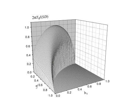
FIG. 14.: 3$d$ plot of $T_{0}(h_{x},h_{z})$. In the main part of the interval $0\leq h_{z}\leq 1$ the transition temperature $T_{0}$ scales with $\delta\equiv 1-h_{z}$.

\begin{picture}(11.0,7.0)\centerline{\hbox{\psfig{angle=-90,width=341.43306pt}}} \end{picture}

FIG. 15.: Dependence $T_{0}(h_{x})$ in the strongly biased case (cf. Fig.  6). Asymptotes based on Eqs.  (1), (91), and (94), on the left side, and on Eqs.  (2) and (105), on the right side, are shown by the dotted lines. The analytically calculated values of Eqs. (113)–(115) are shown by diamonds.

In the general biased case simple analytical results for the quantum-classical transition temperature $T_{0}$ can be obtained in two limiting cases: for small transverse fields and for the fields near the metastability boundary curve. In the first case the quantum-classical transition is of the first order, and a good estimation of the transition temperature $T_{0}$ is given by Eq.  (1), where in the exponential approximation $B=S(U_{\rm min})$. The analytical expression for the bottom-level action $S(U_{\rm min})$ can be found for small $h_{x}$ and arbitrary $h_{z}$ from the general formula (22). In the most interesting strongly biased case this can be done for the arbitrary $h_{x}<h_{xm}$ with the result

$$S(U_{\rm min})\cong 2S\sqrt{2h_{x}y_{\rm min}^{\prime}}\big{[}-3\sqrt{1-r_{\rm min}}$$ (92)

$$\qquad\qquad{}+(r_{\rm min}+2){\rm arctanh}\sqrt{1-r_{\rm min}}\big{]},$$ (93)

where $r_{\rm min}\equiv y_{\rm min}/y_{\rm min}^{\prime}<1$ and $y_{\rm min}^{\prime}\equiv\exp(x_{\rm min}^{\prime})$ is the turning point on the right side of the barrier corresponding to the energy $u_{\rm min}$ of Eq.  (89). For $h_{x}\ll h_{xm}$ one has $y_{\rm min}^{\prime}\cong[\delta^{2}/(2h_{x})](1-h_{x}^{2}/\delta^{3})$ and $r_{\rm min}\cong h_{x}^{2}/\delta^{3}\ll 1$. In this case Eq.  (92) simplifies to

$$S(U_{\rm min})\cong 2S\delta\left\{\ln\left[\frac{27}{2e^{3}}\left(\frac{h_{xm}}{h_{x}}\right)^{2}\right]+\frac{22}{27}\left(\frac{h_{x}}{h_{xm}}\right)^{2}\right\}.$$ (94)

It is instructive to find $S(U_{\rm min})$ for small $h_{x}$ in the whole range of $h_{z}$ with the use of the general perturbative expression for the level splitttings in the biased case [86, 60]

$$\Delta E_{mm^{\prime}}=\frac{2D}{[(m^{\prime}-m-1)!]^{2}}$$ (95)

$$\qquad\times\sqrt{\frac{(S+m^{\prime})!(S-m)!}{(S-m^{\prime})!(S+m)!}}\left(\frac{H_{x}}{2D}\right)^{m^{\prime}-m}$$ (96)

[cf. Eq. (43)], where $m<0$ and $m^{\prime}=-m-H_{z}/D$ is the matching level on the other side of the barrier. For the ground-state level in the metastable well one has $m=-S$ and $m^{\prime}=S(1-2h_{z})$. Now, in the exponential approximation, one can use, according to Eq.  (26), $S^{\rm pert}(U_{\rm min})\cong-2\ln\Delta E_{-S,S(1-2h_{z})}$. Then with the help of the Stirling formula $n!\cong(n/e)^{n}$ one arrives at the result

$$S^{\rm pert}(U_{\rm min})\cong 2S\{\delta\ln[4\delta^{3}/(eh_{x})^{2}]+h_{z}\ln h_{z}\}.$$ (97)

One can check that in the unbiased case ($h_{z}=0$, i.e., $\delta=1$) the first (perturbative) term of Eq. (51) is reproduced, and in the strongly biased case that of Eq.  (94) is recovered. The accuracy of Eq.  (97) is not so high as that of Eq.  (94), which contains the important correction term quadratic in $h_{x}/h_{xm}$. Finally, in the strongly biased case the estimation of the escape-rate transition temperature for small transverse fields is $T_{0}\cong T_{0}^{(0)}=\Delta U/S(U_{\rm min})$ with $\Delta U$ and $S(U_{\rm min})$ given by Eqs.  (91) and (94).

Near the metastability boundary curve the consideration begins with the location of the latter from the conditions $u^{\prime}(x_{m})=0$ and $u^{\prime\prime}(x_{m})=0$, which yields the equations

$$\cosh^{3}(x_{m})=\frac{1}{h_{xm}},\qquad\sinh^{3}(x_{m})=-\frac{h_{zm}}{h_{xm}},$$ (98)

where from Eq.  (10) follows. Then for the field

$$h_{x}=h_{xm}(1-\epsilon_{x}),\qquad h_{z}=h_{zm}(1-\epsilon_{z}),$$ (99)

where $\epsilon_{x,z}\ll 1$ and $\{h_{xm},h_{zm}\}$ are related by Eq.  (10), one can expand the potential $u(x)$ of Eq.  (8) near $x_{m}$ in powers of $x-x_{m}$. If $h_{z}$ is not very small, one can restrict oneself to the third-order terms and obtain

$$u(x)\cong u(x_{m})+A_{1}(x-x_{m})-A_{3}(x-x_{m})^{3}$$ (100)

with

$$A_{1}=2\bar{\epsilon}h_{xm}^{2/3}h_{zm}^{1/3},\qquad A_{3}=h_{xm}^{4/3}h_{zm}^{1/3},$$ (101)

and

$$\bar{\epsilon}\equiv h_{xm}^{2/3}\epsilon_{x}+h_{zm}^{2/3}\epsilon_{z}.$$ (102)

The cubic parabola (100) is symmetric about $x_{m}$ and it is characterized by the barrier height

$$\Delta U=4S^{2}D(2\bar{\epsilon}/3)^{3/2}(h_{xm}h_{zm})^{2/3}$$ (103)

and the equal real and instanton oscillation frequencies

$$\omega_{0}=\tilde{\omega}_{0}=2SD(6\bar{\epsilon})^{1/4}h_{xm}^{1/2}h_{zm}^{1/6},$$ (104)

where the latter defines the quantum-classical transition temperature: $T_{0}=T_{0}^{(2)}=\tilde{\omega}_{0}/(2\pi)$. Equation (104) can be put into the form

$$\omega_{0}=\tilde{\omega}_{0}=2SD(6\bar{\epsilon})^{1/4}\cot^{1/6}\theta_{H}/(1+\cot^{2/3}\theta_{H}),$$ (105)

if one sets $h_{xm}=h_{m}\sin\theta_{H}$ and $h_{zm}=h_{m}\cos\theta_{H}$, where, by virtue of Eq.  (10), $h_{m}=(\sin^{2/3}\theta_{H}+\cos^{2/3}\theta_{H})^{-3/2}$. If, as in Ref. [85], the field changes along the line $\theta_{H}={\rm const}$, one has $\epsilon_{x}=\epsilon_{z}=\epsilon$, which results in $\bar{\epsilon}=\epsilon$. In this case Eq.  (18) of Ref.  [85] is recovered, where, by definition, $\omega_{0}$ is twice as small as here. In the strongly biased case, however, it is more convenient to have $h_{z}$ fixed and swipe $h_{x}$ across the narrow region where the barrier exists. Thus one can set $h_{zm}\cong 1$, $h_{xm}\cong(2\delta/3)^{3/2}$, $\epsilon_{z}=0$, and $\bar{\epsilon}=h_{xm}^{2/3}\epsilon_{x}=(2\delta/3)\epsilon_{x}$ to obtain

$$\Delta U=(16S^{2}D/9)(2\epsilon_{x}/3)^{3/2}\delta^{2}$$ (106)

and

$$\omega_{0}=\tilde{\omega}_{0}=(4SD/3)(6\epsilon_{x})^{1/4}\delta.$$ (107)

Note that at the applicability boundary of the present aproach, $\epsilon_{x}=1$, one has $\Delta U=0.97S^{2}D\delta^{2}$, which is very close to the exact value $\Delta U=S^{2}D\delta^{2}$ for $h_{x}\ll h_{xm}$ obtained above (see Fig.  11). That is, the barrier height scales as $\Delta U\propto\delta^{2}$ in the strongly biased case $\delta\ll 1$. Similarly, the quantum-classical transition temperature scales as $T_{0}\propto\delta$. In fact, as will be shown by the numerical calculations below, this scaling holds not only in the strongly biased case, but practically in the whole region of $h_{z}$, excluding that of very small $h_{z}$.

As a pendant to Eq.  (92), one can calculate the real-time action given by Eq.  (57) for the energy $U_{\rm sad}$ in the strongly-biased case. The result reads

$$S^{\rm real}(U_{\rm sad})\cong 2S\sqrt{2h_{x}y_{\rm sad}^{\prime}}\big{[}-3\sqrt{r_{\rm sad}-1}$$ (108)

$$\qquad\qquad{}+(r_{\rm sad}+2)\arctan\sqrt{r_{\rm sad}-1}\big{]},$$ (109)

where $r_{\rm sad}\equiv y_{\rm sad}/y_{\rm sad}^{\prime}>1$ and $y_{\rm sad}^{\prime}\equiv\exp(x_{\rm sad}^{\prime})$ is the turning point on the left side of the metastable well corresponding to the energy $u_{\rm sad}$ of Eq.  (89). The top-level real-time action above determines according to Eq.  (58) the number of levels in the well. For $h_{x}\ll h_{xm}$ one has $y_{\rm sad}^{\prime}\cong h_{x}/(4\delta)$ and $r_{\rm sad}\cong(2\delta)^{3/2}/h_{x}\gg 1$. Thus in this limit

$$S^{\rm real}(U_{\rm sad})\cong 2\pi S\delta[1-8/(3^{3/4}\pi)\sqrt{h_{x}/h_{xm}}]$$ (110)

[cf. Eq.  (94)] and $N_{\rm lev}=S\delta$ for $h_{x}=0$. Near the metastability boundary the potential $u(x)$ can be approximated by the cubic parabola (100). From Eq.  (98) one obtains $y_{\rm min}^{\prime}\cong y_{\rm sad}^{\prime}\cong\exp(x_{m})=(1-h_{zm}^{1/3})/h_{xm}^{1/3}\cong\delta/(3h_{xm}^{1/3})$. More accurately, $x_{\rm sad,min}\cong x_{m}\pm\sqrt{A_{1}/(3A_{3})}=x_{m}\pm\sqrt{2\epsilon_{x}/3}$ and $x_{\rm sad,min}^{\prime}\cong x_{m}\mp 2\sqrt{2\epsilon_{x}/3}$. This yields $1-r_{\rm min}=1-\exp(x_{\rm min}-x_{\rm min}^{\prime})\cong\sqrt{6\epsilon_{x}}$, and the same for $r_{\rm sad}-1$. Expanding now Eqs.  (92) and (108) for $\epsilon_{x}\ll 1$ results in

$$S(U_{\rm min})\cong S^{\rm real}(U_{\rm sad})\cong(16S\delta/45)(6\epsilon_{x})^{5/4}.$$ (111)

The behavior of $S(U_{\rm min})$ and $S^{\rm real}(U_{\rm sad})$ given by Eqs.  (92) and (108) in the strongly biased case in the whole range of $h_{x}/h_{xm}$ is shown in Fig.  12.

The order of the quantum-classical escape-rate transition is determined, as we have seen, by the sign of the the coefficient $b$ in the expansion of the imaginary-time action $S(E)$ near the top of the barrier [see Eqs.  (46) and (68)]. In the general biased case this coefficient is given by

$$b=\frac{\Delta U}{(2m)^{3}2\tilde{\omega}_{0}^{6}}\left[U_{\rm sad}^{\prime\prime}U_{\rm sad}^{\prime\prime\prime\prime}-\frac{5}{3}(U_{\rm sad}^{\prime\prime\prime})^{2}\right]$$ (112)

[see Eqs.  (2) and (4)]. It reduces to that of Eq.  (47) in the case $h_{z}=0$ where $U_{\rm sad}^{\prime\prime\prime}=0$. In the strongly biased case the potential of the spin system simplifies to Eq.  (86), and there is a simple analytical solution for the line $h_{xc}(h_{z})$ separating the first- and second-order escape-rate transitions. To obtain this line, one can calculate all needed derivatives of $u(x)$ at the top of the barrier from Eq.  (86), equate $b=0$ in Eq.  (112), and eliminate the terms with $h_{x}$ with the help of the relation $h_{x}e^{-2x}=2(-2e^{x}+\delta e^{-x})$ following from $u_{\rm sad}^{\prime}=0$. Then the condition $b=0$ yields $e^{2x}=\delta/\sqrt{6}$, and for $h_{x}=h_{xc}$ one finds

$$h_{xc}\cong(2/3)^{3/4}(\sqrt{3}-\sqrt{2})\delta^{3/2}\cong 0.2345\delta^{3/2},$$ (113)

i.e., $h_{xc}\cong 0.4308h_{xm}$. Further, for $h_{x}=h_{xc}$ one has $u_{\rm sad}^{\prime\prime}\cong-2\delta^{2}(4\sqrt{2/3}-3)$ resulting in the transition temperature at the boundary between first-and second-order transitions

$$T_{0}^{(c)}=(SD/\pi)(4\sqrt{2/3}-3)^{1/2}\delta,$$ (114)

where $(4\sqrt{2/3}-3)^{1/2}\cong 0.5157$ [see Eq.  (2), cf. Eq.  (69)].

The maximum of $T_{0}$ is attained within the range of transverse fields corresponding to the second-order escape-rate transition. In the unbiased case Eq.  (69) yields evidently $T_{0}^{(\rm max)}=SD/(2\pi)$ for $h_{x}=h_{x}^{(\rm max)}=0.5$. In the strongly biased case using the conditions $du^{\prime\prime}[h_{x},x(h_{x})]/dh_{x}=0$ and $u^{\prime}[h_{x},x(h_{x})]=0$ for $x(h_{x})$ corresponding to the maximum of the potential (86) one obtains $e^{2x}=\delta/3$ and

$$T_{0}^{(\rm max)}=(SD/\pi)\delta/\sqrt{3}$$ (115)

for $h_{x}^{(\rm max)}=h_{xm}/\sqrt{2}\cong 0.3849\delta^{3/2}$.

Numerical calculation of the escape rate $\Gamma$ in the general biased case in the exponential approximation poses no problems. The minimum of the effective free energy $F(E)$ of Eq.  (65) with respect to $E$ can be found using the imagimary-time action $S(E)$ numerically calculated from Eq.  (22). For any field ${\bf H}$ one can establish the transition temperature $T_{0}$, such as for $T<T_{0}$ the minimum of $F(E)$ no longer corresponds to the top of the barrier, as it is in the classical case. Analyzing the dependence $F(E)$ for different fields allows one to determine the order of the quantum-classical escape-rate transition (see Fig.  5). The boundary between the first- and the second-order transitions can be found the most easily from the condition $b=0$ in Eq.  (112), where the derivatives of $U(x)$ are calculated at the numerically determined top of the barrier. This method yields the same results for $h_{xc}(h_{z})$ as that described above. The resulting phase diagram for the escape-rate transition is shown in Fig.  13. The 3$d$ plot of $T_{0}(h_{x},h_{z})$ is shown in Fig.  14. The dependence $T_{0}(h_{x})$ in the strongly-biased case is given in Fig.  15.

V Discussion

We have presented a comprehensive study of the thermal and quantum decay of a metastable spin state of the uniaxial spin system in the arbitrarily directed magnetic field. The moderate damping regime has been studied, in which the damping does not influence the dynamics of the spin system but provides the thermal equilibrium with the environment. The method employed is the mapping of a spin system onto the particle in a double-well potential, with the subsequent use of the WKB approach. The explicit dependence of the escape rate, including the prefactor, on temperature, field, and anisotropy constant has been worked out and compared with limiting cases obtained by others. This calculation shows how formulas describing different regimes join on temperature down to lowest temperatures where quantization of levels becomes significant. The crossover from thermally assisted tunneling to the ground-state tunneling at $T\sim T_{00}$ is described quantitatively and discussed in detail [see Eqs.  (81) and (82)]. The fascinating new feature of this analysis is the existence for spin systems of both, first- and second-order, transitions from thermal activation to thermally assisted tunneling at $T=T_{0}$. The kind of transition depends on the strength and the direction of the magnetic field. We have calculated the boundary in the $H_{x},H_{z}$ plane separating the two different regimes.

The direct analogy with phase transitions exists in the limit of a very large spin $S$. In that limit the dependence of the transition rate on temperature changes abruptly at $T_{0}$, pretty much as thermodynamic quantities do in the theory of phase transitions. For finite $S$, both the first- and second-order transitions of the escape rate are smeared, similar to the smearing of the phase transition in a finite-size system. The reduced width of the crossover between the classical and quantum regimes $\Delta T/T_{0}$ is of the order of $S^{-1/2}$ for the second-order transition and $S^{-1}$ for the first-order transition.

For a moderately large spin, $S\sim 10$, one can explore in experiment the entire phase diagram shown in Fig.  13. This is the case of molecular magnets like Mn₁₂Ac. If greater spins are studied, the external magnetic field must be adjusted such that the energy barrier becomes small enough to provide a significant tunneling rate. In terms of the phase diagram this means that one has to work close to the metastability boundary line, Eq.  (10), separating the field ranges with and without the barrier. According to Fig.  13, for a uniaxial spin close to the metastability boundary, both, first- and second-order, transitions coexist only in the lower right corner of the phase diagram. In this region, close to the boundary between first- and second-order transitions, the temperature $T_{0}$ is of order $BD/(4\pi^{2})$, where $B$ is the exponent in the expression for the rate. In a typical tunneling experiment with a macroscopic lifetime of a metastable state, $B\sim 4\pi^{2}$, so that $T_{0}\sim D$. The latter constant can be expressed in terms of the anisotropy field and the total spin of the particle: $D=g\mu_{B}H_{A}/(2S)$. For $H_{A}\sim 1$ T and $S\sim 100$ the transition temperature will be of the order of 10 mK. This is within experimental reach. Notice that the smallness of $T_{0}$ in our model comes, in part, from the fact that the noncommutation of $S_{z}$ with the Hamiltonian is small in the lower right corner of the phase diagram, where the effect is to be searched for. One can expect that in models with transverse anisotropy observable first- and second-order transitions will coexist at higher temperatures, since the transverse anisotropy, rather than the required small transverse field, will drive the decay of the metastable state. Such a model requires a different approach and will be worked out elsewhere.

REFERENCES

- [1]
-
[2]
Permanent address: I. Institut für Theoretische Physik, Universität Hamburg,
Jungiusstrasse 9, D-20355 Hamburg, Germany.
Electronic addresses: garanin@physnet.uni-hamburg.de
garanin@mpipks-dresden.mpg.de
http://www.mpipks-dresden.mpg.de/garanin/ - [3] Permanent address: Departament de Física Fonamental, Universitat de Barcelona, Av. Diagonal 647, 08028 Barcelona, Spain Electronic address: xavim@hermes.ffn.ub.es
-
[4]
Electronic address: chudnov@lcvax.lehman.cuny.edu
- [5] F. Hund, Z. Phys. 43, 805 (1927).
- [6] G. Wentzel, Z. Phys. 38, 518 (1926).
- [7] H. A. Kramers, Z. Phys. 39, 828 (1926).
- [8] L. Brillouin, C. R. Acad. Sci. Paris 183, 24 (1926).
- [9] J. R. Oppenheimer, Phys. Rev. 31, 80 (1928).
- [10] R. H. Fowler and L. Nordheim, Proc. R. Soc. London, Ser. A 119, 173 (1928).
- [11] G. Gamov, Z. Phys. 51, 204 (1928).
- [12] I. Ya. Korenblit and E. F. Shender, Zh. Eksp. Teor. Fiz. 75, 1862 (1978) [JETP 48, 937 (1978)].
- [13] E. M. Chudnovsky, Zh. Eksp. Teor. Fiz. 77, 2157 (1979) [JETP 50, 1035 (1979)].
- [14] M. Enz and R. Schilling, J. Phys. C 19, L711 (1986).
- [15] E. M. Chudnovsky and L. Gunther, Phys. Rev. Lett. 60, 661 (1988).
- [16] J. L. van Hemmen and A. Sütő, Physica B 141, 37 (1986).
- [17] H. A. Kramers, Physica 7, 284 (1940).
- [18] E. C. Stoner and E. P. Wohlfart, Philos. Trans. R. Soc. London, Ser. A 240, 599 (1948); reprinted in: IEEE Trans. Magn. MAG-27, 3475 (1991).
- [19] L. Néel, Ann. Geophys. (C.N.R.S.) 5, 99 (1949).
- [20] W. F. Brown, Jr., Phys. Rev. 130, 1677 (1963).
- [21] P. Hänggi, P. Talkner, and M. Borkovec, Rev. Mod. Phys. 62, 251 (1990).
- [22] P. C. E. Stamp, E. M. Chudnovsky, and B. Barbara, Int. J. Mod. Phys. B 6, 1355 (1992).
- [23] W. T. Coffey, Yu. P. Kalmykov, and J. T. Waldron, The Langevin Equation (Word Scientific, Singapore, 1996).
- [24] D. D. Awshalom, J. F. Smyth, G. Grinstein, D. P. DiVincenzo, and D. Loss, Phys. Rev. Lett. 68, 3092 (1992).
- [25] S. Gider, D. D. Awshalom, T. Douglas, S. Mann, and M. Chaprala, Science 268, 77 (1995).
- [26] J. Tejada, X. X. Zhang, E. del Barco, J. M. Hernández, and E. M. Chudnovsky, Phys. Rev. Lett. 79, 1754 (1997).
- [27] W. Wernsdorfer, E. Bonet Orozco, K. Hasselbach, A. Benoit, D. Mailly, O. Kubo, H. Nakano, and B. Barbara, Phys. Rev. Lett. 79, 4014 (1997).
- [28] M. A. Novak and R. Sessoli, in Quantum Tunneling of Magnetization, edited by L. Gunther and B. Barbara (Kluwer, Dordrecht, 1995).
- [29] B. Barbara et. al., J. Magn. Magn. Mater. 140-144, 1825 (1995).
- [30] J. R. Friedman, M. P. Sarachik, J. Tejada, and R. Ziolo, Phys. Rev. Lett. 76, 3830 (1996).
- [31] J. M. Hernández, X. X. Zhang, F. Luis, J. Bartolomé, J. Tejada, and R. Ziolo, Europhys. Lett. 35, 301 (1996).
- [32] L. Thomas, F. Lionti, R. Ballou, D. Gatteschi, R. Sessoli, and B. Barbara, Nature (London) 383, 145 (1996).
- [33] P. C. E. Stamp, Nature (London) 383, 125 (1996); E. M. Chudnovsky, Science 274, 938 (1996); B. Schwarzschild, Phys. Today 50, No. 1, 17 (1997).
- [34] C. Sangregorio, T. Ohm, C. Paulsen, R. Sessoli, and D. Gatteschi, Phys. Rev. Lett. 78, 4645 (1997).
- [35] V. I. Goldanskii, Dokl. Akad. Nauk. SSSR 124, 1261 (1959) [Sov. Phys. Dokl., 4, 74 (1959)].
- [36] R. P. Bell, Trans. Faraday Soc. 55, 1 (1959); The Tunnel Effect in Chemistry (Chapman and Hall, London, 1980).
- [37] I. Affleck, Phys. Rev. Lett. 46, 388 (1981).
- [38] A. O. Caldeira and A. J. Leggett, Ann. Phys. (N.Y.) 149, 374 (1983).
- [39] H. Grabert and U. Weiss, Phys. Rev. Lett. 53, 1787 (1984).
- [40] H. Grabert, P. Olschowski, and U. Weiss, Phys. Rev. B 32, 3348 (1985).
- [41] A. I. Larkin and Yu. N. Ovchinnikov, Zh. Eksp. Teor. Fiz. 86, 719 (1984) [JETP 59, 420 (1984)].
- [42] W. Zwerger, Phys. Rev. A 31, 1745 (1985).
- [43] P. S. Riseborough, P. Hänggi, and E. Freidkin, Phys. Rev. A 32, 489 (1985).
- [44] A. I. Larkin and Yu. N. Ovchinnikov, Pis’ma Zh. Eksp. Teor. Fiz. 37, 322 (1983) [JETP Lett. 37, 382 (1983)].
- [45] E. M. Chudnovsky, Phys. Rev. A 46, 8011 (1992).
- [46] E. M. Chudnovsky and D. A. Garanin, Phys. Rev. Lett. 79, 4469 (1997).
- [47] L. D. Landau, Z. Phys. Sowjet. 11, 26 (1937).
- [48] C. Morais-Smith, B. Ivlev, and G. Blatter, Phys. Rev. B 49, 4033 (1994).
- [49] J. Garriga, Phys. Rev. D 49, 5497 (1994).
- [50] A. Ferrera, Phys. Rev. D 52, 6717 (1995).
- [51] S. Habib, E. Mottola, and P. Tinyakov, Phys. Rev. D 54, 7774 (1996).
- [52] F. Zimmerschied, D. H. Tchrakian, and H. J. W. Müller-Kirsten, Forschritte der Physik 46 147 (1998).
- [53] M. A. Skvortsov, Phys. Rev. B 55, 515 (1997).
- [54] D. A. Gorokhov and G. Blatter, Phys. Rev. B 56, 3130 (1997).
- [55] G. Scharf, Ann. Phys. (N.Y.) 83, 71 (1974).
- [56] O. B. Zaslavskii, V. V. Ulyanov, and V. M. Tsukernik, Fiz. Nizk. Temp. 9, 511 (1983) [Sov. J. Low Temp. Phys. 9, 259 (1983)].
- [57] G. Scharf, W. F. Wreszinski, and J. L. van Hemmen, J. Phys. A: Math. Gen. 20, 4309 (1987).
- [58] O. B. Zaslavskii, Phys. Lett. A 145, 471 (1990).
- [59] O. B. Zaslavskii, Phys. Rev. B 42, 992 (1990).
- [60] D. A. Garanin and E. M. Chudnovsky, Phys. Rev. B 56, 11102 (1997).
- [61] J. Villain, F. Hartmann-Boutron, R. Sessoli, and A. Rettori, Europhys. Lett. 27, 159 (1994).
- [62] D. A. Garanin, Phys. Rev. E 55, 2569 (1997).
- [63] L. D. Landau and E. M. Lifshitz, Z. Phys. Sowjet. 8, 153 (1935).
- [64] T. L. Gilbert, unpublished report; mentined in: Phys. Rev. 100, 1243 (1955).
- [65] D. A. Smith and F. A. de Rozario, J. Magn. Magn. Mater. 3, 219 (1976).
- [66] W. F. Brown, Jr., IEEE Trans. Magn. MAG-15, 1196 (1979).
- [67] I. Klick and L. Gunther, J. Stat. Phys. 60, 473 (1990).
- [68] L. J. Geoghegan, W. T. Coffey, and B. Mulligan, Adv. Chem. Phys. 100, 475 (1997).
- [69] W. T. Coffey, D. S. F. Crothers, J. L. Dormann, L. J. Geoghegan, and E. C. Kennedy, J. Magn. Magn. Mater. 173 L219 (1997).
- [70] W. Wernsdorfer, E. Bonet Orozco, K. Hasselbach, A. Benoit, B. Barbara, N. Demoncy, A. Loiseau, and D. Mailly, Phys. Rev. Lett. 78, 1791 (1997).
- [71] M. Razavy, Am. J. Phys. 48, 285 (1980).
- [72] L. D. Landau and E. M. Lifshitz, Quantum Mechanics (Pergamon, London, 1965).
- [73] E. C. Kemble, Phys. Rev. 48, 549 (1935).
- [74] U. Weiss and W. Haeffner, Phys. Rev. D 27, 2916 (1983).
- [75] H. K. Shepard, Phys. Rev. D 27, 1288 (1983).
- [76] A. Garg, Phys. Rev. B 51, 15161 (1995).
- [77] A. Garg and G.-H. Kim, Phys. Rev. Lett. 63, 2512 (1989); Phys. Rev. B 43, 712 (1991).
- [78] R. Rose, S. Han, and J. E. Lukens, Phys. Rev. Lett. 75, 1614 (1995).
- [79] P. Silvestrini, V. G. Palmieri, B. Ruggiero, and M. Russo, Phys. Rev. Lett. 79, 3046 (1997).
- [80] A. Aharoni, Phys. Rev. 177, 793 (1969).
- [81] P. F. Byrd and M. D. Friedman, Handbook of Elliptic Integrals for Engineers and Scientists (Springer, New York, 1979).
- [82] D. A. Garanin, J. Phys. A: Math. Gen. 24, L61 (1991).
- [83] F. Hartmann-Boutron, J. Phys. I 5, 1281 (1995).
- [84] R. P. Feynman, Statistical Mechanics (Benjamin, New York, 1972).
- [85] M.-Carmen Miguel and E. M. Chudnovsky, Phys. Rev. B 54, 388 (1996).
- [86] E. M. Chudnovsky and J. R. Friedman, (unpublished).