Phase behavior of a system of particles with core collapse

Abstract

The pressure-temperature phase diagram of a one-component system, with particles interacting through a spherically symmetric pair potential in two dimensions is studied. The interaction consists of a hard core plus an additional repulsion at low energies. It is shown that at zero temperature, instead of the expected isostructural transition due to core collapse occurring when increasing pressure, the system passes through a series of ground states that are not triangular lattices. In particular, and depending on parameters, structures with squares, chains, hexagons and even quasicrystalline ground states are found. At finite temperatures the solid-fluid coexistence line presents a zone with negative slope (which implies melting with decreasing in volume) and the fluid phase has a temperature of maximum density, similar to that in water.

]

I Introduction

Determination of the phase structure of real materials from first principles calculations has been one of the aims of statistical mechanics since long ago. Although a qualitative understanding of the processes leading to the different kinds of phase transitions (between gas, liquid, and one or more solid phases) in the pressure-temperature ($P$-$T$) phase diagram of a classical system has been gained, it is clear that the quantitative fitting of the behavior of real materials requires a detailed knowledge of the interaction between particles and a great deal of computational work, that only in recent years has become feasible.

In addition to the usual materials in which atoms or molecules are the basic constituents, in the last years colloidal dispersions have provided a new kind of systems in which parameters such as particle size and interaction potential can be varied greatly.[2] These systems consist of a set of latex spheres in colloidal suspension, with the aggregate of some amount of non-adsorbing polymer, which modifies the interaction potential between the particles. Their study has practical importance in relation to the properties of many common substances (such as ink, paints, cosmetics, blood, etc.). It is clear that a knowledge of the phase behavior of different model systems is important in order to compare the theoretical predictions with the experimental results.

Much effort has been spent in the elucidation of the properties of binary mixtures of particles of two different sizes, where segregation, flocculation, partial crystallization and other phenomena may occur.[3] On the other hand, other studies have been directed towards the determination of the phase behavior of identical particles interacting through different model potentials. In this case the possibilities for the behavior of the system are not so wide as in the case of binary mixtures but, however, interesting phenomena occur. It was shown for instance, that the usual solid-liquid-gas phase diagram of particles interacting through a hard core repulsion plus a long range attraction is modified when the range of the attraction is decreased.[4] More precisely, the liquid-gas coexistence curve disappears if the range of the attractive potential is lower than about 30% of the hard core radius. More interestingly, when the range of the attractive potential is reduced below about 8% of the repulsive range, a coexistence curve separating two isostructural solid phases appear.

A more obvious isostructural transition occurs in the case in which the attractive well is replaced by a repulsive shoulder. In this case, for low pressures, the repulsive shoulder can sustain a compact structure with a lattice parameter related to its range. But when applying enough pressure the system must collapse to a new compact structure with a lattice parameter given by the real hard core of the particles. This kind of models, whether with a square shoulder, or a linear ramp soft core (which is the one discussed in this paper) have been studied since long time ago with the picture of core collapse in mind.[5] Extensions to more general potential were also performed.[6] In recent papers the problem has been revisited, and in particular the isostructural transition has been studied numerically,[7] and analytical results have shown that in three dimensions, the ground state of a system with a hard core plus a repulsive shoulder can be one of various crystalline structures depending on parameters.[8]

In this paper I show for the hard core plus linear ramp model in two dimensions that even the stable zero temperature structures may be very different from the expected triangular structures. The most stable configuration may be one of a variety of crystalline structures, and even a quasicrystal. These structures melt when increasing temperature. The solid-fluid border in the $P$-$T$ diagram has a zone with negative slope, which implies a melting with decreasing in volume and in this region the fluid has an anomalous thermal expansion,[9] up to a temperature at which a density maximum is attained.

The paper is organized as follows. In the next section the model is introduced and details of the simulation procedure to be used in Section IV are provided. In Section III the ground state configurations are analyzed. In section IV, I present detailed results for the $P$-$T$ phase diagram for a particular value of the parameter $\alpha,$ which is defined below. In Section V, possible relevance to real systems are discussed and a summary of the results is given.

II Model and numerical technique

The model interaction $U\left(r\right)$ between particles that will be used here consists of a hard core repulsion at a radius $r_{0}$ ($U\left(r\right)|_{r<r_{0}}=\infty$), is zero for distances larger than a value $r_{1}$, and has a soft repulsive part for $r_{0}<r<r_{1}$ of the form $U\left(r\right)=\varepsilon_{0}\left(r_{1}-r\right)/\left(r_{1}-r_{0}\right)$ (Figure 1). This interaction gives a model that is a candidate to have an isostructural transition between compact configurations of lattice parameter $r_{0}$ and $r_{1}.$ Two particles interacting through this potential in the presence of an external force $f$ trying to bring them together, will have a jump in the interparticle distance from $r_{1}$ to $r_{0}$ when $f$ exceeds the critical value $\varepsilon_{0}/\left(r_{1}-r_{0}\right).$ This model is preferred for numerical simulations instead of the square shoulder model, because it has much less metastabilities when varying pressure or temperature. If temperature is measured in units of the energy at contact $\varepsilon_{0}$ (Boltzmann constant is taken to be 1), and distances in units of the hard core distance $r_{0}$, then $\alpha=r_{1}/r_{0}$ is the only free parameter of the interaction potential.

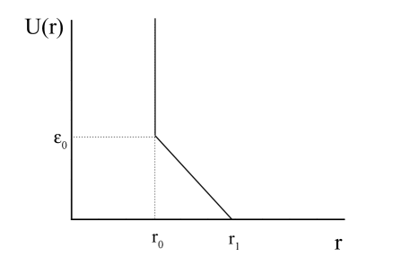
FIG. 1.: The pair potential used throughout the paper. There is a hard core at distance $r_{0}$ and a soft core (linear ramp) between $r_{0}$ and $r_{1}$. Interaction vanishes beyond $r_{1}$.

Detailed numerical simulations were performed for a two-dimensional system of 256 particles in the NPT ensemble, using the Montecarlo-Metropolis technique. A trial movement of a particle consists of a displacement to a new position chosen randomly inside a cube of a linear size of 1% of the mean distance between particles. The new position is accepted with a Metropolis algorithm, considering the energy change due to the movement. Once each five Montecarlo swepts through all particles, a trial global rescaling of all particle coordinates and system size is proposed. The rescaling is given by a factor chosen randomly within the interval $\pm 0.2\%$, and is done independently for $x$ and $y$ coordinates, in order to allow the system to accommodate the different crystalline structures that may appear. A maximum aspect ratio for the system of 1.05 is imposed. If the trial volume change does not produce hard core particle overlapping, then it is accepted according to the Metropolis rule with the value of the energy change $\Delta E$, given by $\Delta E=P\Delta V-\left(NT/V\right)\Delta V+dE$. Here $N$ is the number of particles, $V$ the volume of the system, $dE$ is the energy change associated to the change of interparticle distances, and the term $-\left(NT/V\right)\Delta V$ $-$which assures the correct limiting equation of state in the case of an ideal gas (i.e., when $dE=0$)$-$ accounts for the kinetic energy term that $-$as usual$-$ can be integrated out in the expression for partition function and thermodynamic potentials. Different runs were performed at constant pressure starting from random configurations at high temperature, cooling down to zero temperature and then warming up. Around 10000 Montecarlo steps were used for thermalization at each temperature, and then 50000 steps were used to calculate thermodynamic quantities, such as the mean volume $v$ per particle at each temperature, the enthalpy per particle $h$, the diffraction pattern of the geometrical configurations, and the diffusion coefficient of the particles $D$.

The diffusion coefficient is calculated in the following way. The distance traveled by each particle, starting from its initial position, as a function of time is recorded, and $D$ is taken to be the slope of this function at long times. From this definition and the kind of simulations performed, it is clear that $D$ tends to a constant at high temperatures. The physical diffusion cefficient is obtained multiplying by temperature. In addition, from the diffraction patterns an orientational order parameter $B_{m}$ will also be used. It is defined as

$$B_{m}=\int K\left(k\right)P(k,\theta)\exp(im\theta)d^{2}{\bf k.}$$ (1)

Here $P\left(k,\theta\right)$ is the intensity of the diffraction pattern in the ${\bf k}$ plane, in polar coordinates, $m$ is an integer chosen according the orientational order we are looking for, and $K\left(k\right)$ is a kernel that cuts off the integral at large $k$. The results are qualitatively insensitive to the form of $K\left(k\right).$ The expression used was $K\left(k\right)=\exp(-k^{2})$.

Some comments are in order at this point. The use of the hard core plus linear ramp potential is motivated $-$as stated before$-$ by numerical reasons. Both the analytical results of the following section and the numerical ones of section III do not change qualitatively if a square shoulder, or a parabolic one (with negative second derivative) is used instead of the linear ramp. More precise conditions on the potential are discussed in Section V. Results are presented for the two-dimensional case to clarify the discussions of the structures that will be presented in the next section. However, the basic properties of the system remain the same in three dimensions. The nature of the melting transition in two dimensions is a controversial point in the literature. However, for rather small systems as the one studied here, indications of discontinuous melting transitions are clearly observed, but is not obvious whether they remain when the system size goes to infinity. I will speak throughout the paper of continuous and discontinuous melting transitions when the simulations indicate each case for the particular size used in the simulations.

III Zero temperature behavior

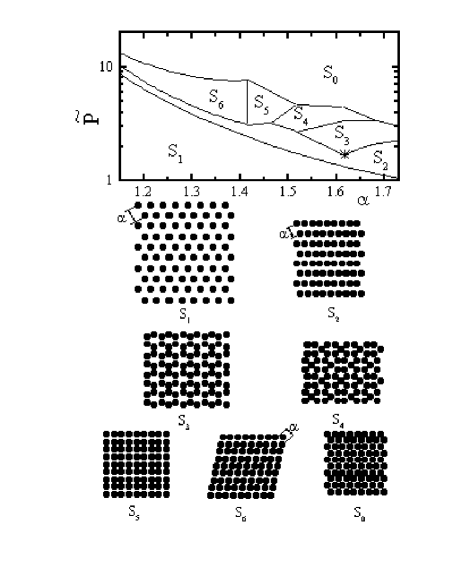
FIG. 2.: Ground state configurations of the system as a function of $\widetilde{P}$ ($\equiv Pr_{0}^{2}/\varepsilon_{0}$) and $\alpha.$ At the point marked by a star, the ground state of the system is a random quasicrystal. The black dots in the configurations represent the hard core of the particles.

Since the first numerical works of Alder and Wainwrigth[10] in the sixties, it has been known that the existence of a high enough external pressure $P$ is sufficient to make a system of otherwise repulsive particles to freeze. The minimum energy configuration of a system of particles interacting in two dimensions through a potential of the form $\sim r^{-\gamma}$ is a triangular lattice for all positive values of $\gamma$. It is not so widely recognized the great variety of ground states that can be obtained for more general potentials, even keeping the restriction of a monotonically decaying potential. We will concentrate in the already introduced hard core plus linear ramp potential (Fig. 1). The ground state configuration of a system of particles in two dimensions interacting through this potential depends on the values of $P$ and $\alpha$, and is not necessarily a triangular lattice.

Depending on pressure, nearest particles tend to be at distance $r_{0}$ or $r_{1}$ from each other. Intermediate values are not preferred because are not energy minima. The origin of complex ground state structures in the system is related to the competition between two terms in the enthalpy $H$ of the system. One is the usual $PV$ term, which tends to minimize the volume, and the other is the repulsive energy term, which tends to maximize the interparticle distance. This produces a sort of frustration, because both terms cannot be minimized at the same time. The two triangular structures with lattice parameters $r_{0}$ and $r_{1}$ (that will be referred to as structures $S_{0}$ and $S_{1}$) correspond to two ways of reducing the enthalpy by minimizing one term whereas maximizing the other. These are the best compromises in the case of very low or very high pressures. However, when both energy terms are comparable, lower energy intermediate solutions can be found by arranging the particles with a coordination number (number of neighbors at distance $r_{0}$) intermediate between 0 and 6 (which correspond to the structures $S_{1}$ and $S_{0}$).

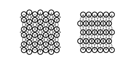
FIG. 3.: Tiling of the structures $S_{3}$ and $S_{2}$ using the two-dimensional Penrose tiles, for $\widetilde{P}=\widetilde{P}_{\text{qc}}$ and $\alpha=\alpha_{\text{qc}}$. The proportion of thin to fat tiles is 1:3 in $S_{3}$ and 2:1 in $S_{2}$. At $\widetilde{P}_{\text{qc}}$, $\alpha_{\text{qc}}$, any possible random tiling of the plane produces a degenerate ground state.

In fact, different crystalline configurations can be proposed, and their enthalpy calculated in order to find the most stable one as a function of $\widetilde{P}$ ($\equiv Pr_{0}^{2}/\varepsilon_{0}$) and $\alpha$. The result of this analysis is shown in Fig. 2. This figure shows the results up to a value of $\alpha$ for which the interaction to second neighbors in the most compact structure ($S_{0}$) is still zero. The structures in Fig. 2 were found by inspection, and they are the lowest energy configurations found within each region, but other (more stable) structures may have been missed. Note that some of the structures have one particle per unit cell (all particles are in translationally equivalent sites), but in others ($S_{3}$ and $S_{4}$) this number is greater than one. For some values of $\alpha$ and as a function of $P$, there are at least three intermediate structure between the triangular ones $S_{0}$ and $S_{1}$.

There is one point in the $\widetilde{P}$-$\alpha$ diagram that deserves further discussion, and this is the one marked by a star in Fig. 2. It corresponds to a value of $\alpha\equiv\alpha_{\text{qc}}=1+2\sin(18^{\text{o}})\cong 1.618$, and $\widetilde{P}\equiv\widetilde{P}_{\text{qc}}=1/\sin(36^{\text{o}})\cong 1.7013$. At this point structures $S_{2}$ and $S_{3}$ become energetically degenerated, but more importantly, many other degenerate structures can be constructed. In fact, structure $S_{3},$ and structure $S_{2}$ for this value of $\alpha$ may be considered as generated by a tiling of the plane using the two 2D Penrose tiles as indicated in figure 3.[11] Particles are located in the far vertices of the thin tile, and in the nearest ones of the fat tile. At the point $S_{\text{qc}}$ the enthalpies per particle of the two Penrose tiles coincide. Any tiling, with the only restriction imposed by the location of the particles in the above mentioned vertices of the tiles (these are usually named soft matching rules and the kind of tiling they generate is known as a random tiling[12, 13]) generates a possible ground state of the system. The proportion of thin to thick tiles used to construct the ground state is arbitrary (as long as the soft matching rules can be satisfied). For proportions close to the value corresponding to a perfect Penrose lattice (nearly 1) the structure obtained is a random quasicrystal. For pressures lower than $\widetilde{P}_{\text{qc}}$ the structure with a maximum fraction of thin tiles ($S_{2}$) is preferred, because the thin tile has lower enthalpy. On the contrary, for pressures higher than $\widetilde{P}_{\text{qc}}$ the preferred structure is that with the largest proportion of fat tiles ($S_{3}$). Quasicrystalline ground states are only stable at the point $S_{\text{qc}}.$ However, the soft matching rules allow for many ways of generating them (compared to the more rigid structures $S_{2}$ and $S_{3}$), and this implies that at finite temperature the quasicrystalline structure will be stabilized due to entropic effects, as we will see in the next section using numerical simulations.

IV Pressure-Temperature phase diagram

After having discussed its ground state properties, we focus now on the behavior of the system at finite temperatures. The main interest is in the localization of the fluid-solid transition line. I will present now the numerical results obtained at different values of pressure, in the particular case $\alpha=1.65$. The system is initialized in a random configuration at high temperature (well inside the fluid phase) and the temperature is progressively reduced to zero, and then increased again.

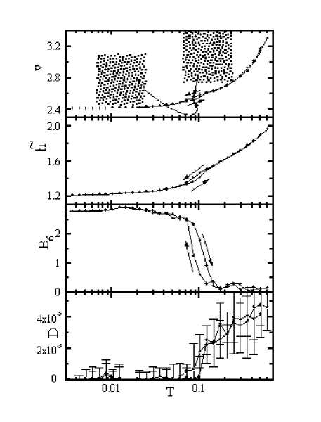
FIG. 4.: Volume $v$, and enthalpy $\widetilde{h}$ ($\equiv E/N+\widetilde{P}v$) per particle, sixfold orientational order parameter $B_{6},$ and diffusion coefficient $D$ of the system as a function of temperature for $\widetilde{P}=0.5$, for a swept decreasing and increasing temperature ($B_{6}$ and $D$ are given in arbitrary units, $T$ is in units of $\varepsilon_{0}$). Note the difference in the snapshots of the system at the same temperature on heating and cooling, within the hysteresis loop.

In the ranges of pressure in which the structures $S_{0}$ and $S_{1}$ are the most stable zero temperature configurations (according to Fig. 2), a sharp solidification transition is obtained when reducing temperature. This can be seen in figures 4,5, and 6 for three different values of pressure within this range. In the first two the solidification is into the $S_{1}$ structure, and for the third one into the $S_{0}$ structure. In the three cases the solidification transition is clearly identifiable by the hysteresis loop in the volume or the enthalpy of the system, which coincides with the vanishing of the diffusion coefficient and the appearance of a finite sixfold symmetry of the diffraction pattern.

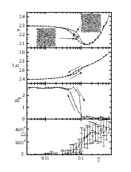
FIG. 5.: Same as Figure 4 for $\widetilde{P}=1.0.$

An additional check of the existence of a sharp solid-fluid transition may be obtained through a long simulation at the equilibrium temperature between solid and fluid. In this case, the volume of the system should fluctuate between two clearly different values corresponding to solid and fluid phases. Results of this simulation are shown for the case $\widetilde{P}=1,$ and $T=0.082$ in Fig. 7. For this simulation the system was initialized in a fluid equilibrium configuration at the corresponding values of $\widetilde{P}$ and $T$. After about 5$\times 10^{5}$ Montecarlo steps the system jumps to the solid phase. After around 2.7$\times 10^{6}$ steps the systems makes a new short transition to the fluid state.

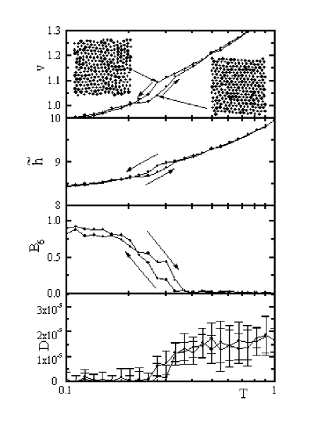
FIG. 6.: Same as Figure 4 for $\widetilde{P}=6.0.$

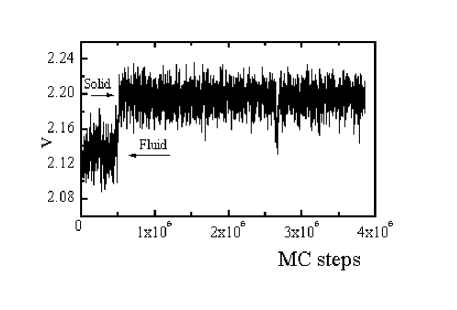
FIG. 7.: Time evolution of the volume per particle $v$ for $\widetilde{P}=1.7$ and $T=0.082,$ close to the fluid-solid transition. After about 5$\times 10^{5}$ Montecarlo steps the system jumps to the solid phase. After around 2.7$\times 10^{6}$ steps the systems makes a new short transition to the fluid state.

The most important characteristic to be noted in Fig.5, is that the melting occurs with a reduction in volume for this value of pressure. In addition, the fluid right after melting has also anomalous thermal expansion up to some temperature at which a density maximum is attained. These characteristics imply a negative slope of the solid-fluid coexistence curve, which is in fact obtained from the simulations as we will see later. The compressive melting of the system in this region has its origin in the fact that the usual volume reduction when temperature is reduced is overcome by the expansion produced when particles diminish their kinetic energy and move out of the soft core of their neighbors. Illustrating this effect, in Fig. 8 we see snapshots of the system at different temperatures passing through the liquid-to-solid transition. In the fluid phase there are particles at distances lower that $r_{1}$ from each other, whereas in the solid phase the minimum distance between particles is $r_{0}$ (except for some defects in the structure, which appear mainly because of the impossibility of accommodate 256 particles in a perfect triangular lattice within a nearly square cage).

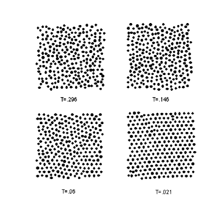
FIG. 8.: Snapshots of the system for $\widetilde{P}=1.7$ when decreasing temperature, through the fluid-solid transition, illustrating the anomalous freezing. In the fluid state there are particles at distance lower than $r_{1},$ whereas in the solid phase all particles (except a few defects) are located at distance $r_{1}$ from their neighbors. The temperature at the second panel corresponds to the maximum density of the system (see Fig. 5).

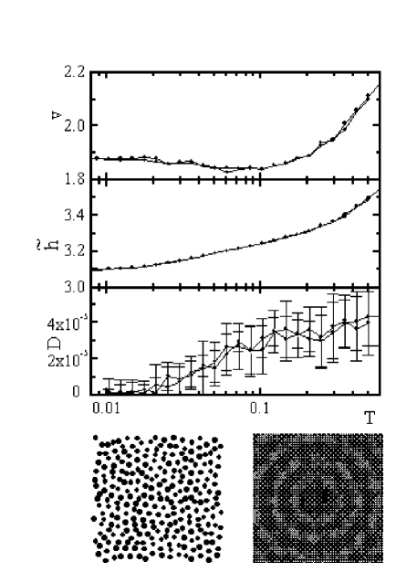
FIG. 9.: Volume per particle $v,$ enthalpy $\widetilde{h}$, and diffusion coefficient $D$ of the system as a function of temperature for $\widetilde{P}=1.3$, for a swept decreasing and increasing temperature. The zero temperature configuration reached and its diffraction pattern are also shown.

The phases $S_{2},$ $S_{3},$ and $S_{4},$ expected to be the ground states of the system at intermediate pressures for $\alpha=1.65$, are not straightforwardly obtained in the simulations. Instead, rather disordered states are obtained. In figures 9, 10, and 11 we can see the magnitudes $v,$ $\widetilde{h},$ and $D$ for pressures $\widetilde{P}=1.3,$ 1.7, and 3.8, together with the zero temperature configuration found and the diffraction pattern of the zero temperature structure. In all the intermediate pressure range ($1.2\lesssim\widetilde{P}\lesssim 4$) the enthalpy at zero temperature obtained in the numerical simulation is never lower than the corresponding to the expected ordered structures of Fig. 2, as it is shown in Fig. 12, indicating that probably the configurations of Fig. 2 are really the fundamental states, but they were not reached in the simulations. The configurations obtained in the simulations reflect the equilibrium states at some finite but small temperature, where entropic contributions to the free energy are important, and they are metastable at zero temperature (note the existence of chains in Fig. 9, and the pentagons and hexagons in Figs. 10 and 11). Looking at the diffraction patterns in Figs. 9, 10, and 11, some of them ($\widetilde{P}=1.3,$ and $\widetilde{P}=3.8$) show no sign of orientational order. Others ($\widetilde{P}=1.7$) clearly indicate a tenfold symmetry, characteristic of a quasicrystal. In the cases where the low temperature state has no orientational order, the volume or enthalpy of the system do not show any abrupt solidification transition. In the cases where the low temperature state has rotational order the volume and enthalpy of the system show a small hysteretic behavior, suggesting an abrupt solidification transition. To confirm this fact, long runs were performed at the expected transition temperature, recording the temporal evolution of volume and enthalpy. An example of the results for the case $\widetilde{P}=1.7$ is shown in Fig. 13. The histogram shows a clear bimodal distribution between two values corresponding precisely to the values of enthalpy expected from Fig. 10 at this temperature.

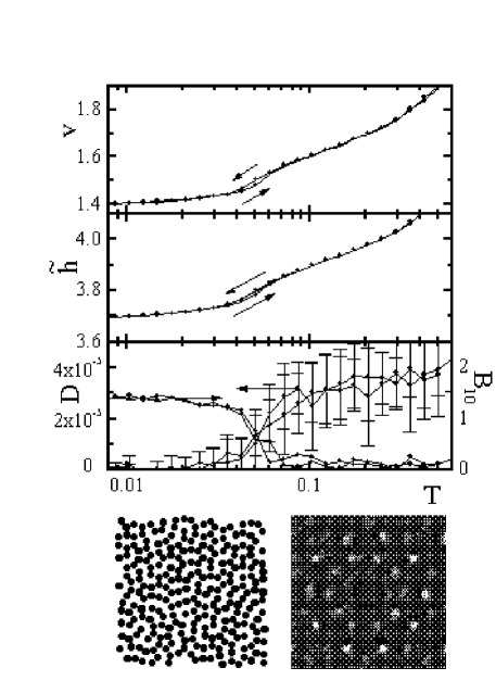
FIG. 10.: Same as Fig. 9 for $\widetilde{P}=1.7$. In this case the tenfold orientational order parameter $B_{10}$ is also shown in the last panel. Note the small histeresis loop in $v$ and $h$.

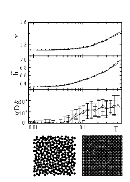
FIG. 11.: Same as Fig. 9 for $\widetilde{P}=3.8$.

We saw in the previous section that at zero temperature the quasicrystalline structure is stable only at a particular value of $\widetilde{P}$ and $\alpha$. At finite temperatures this structure is stabilized due to entropic effects, because there are many ways of construct the random tiling, favoring this structure against the more rigid ones $S_{2}$ and $S_{3}$.[14] A related model of a quasicrystal using two kinds of particles of different sizes has been studied by Strandburg and coworkers.[12, 15] In our case, the quasicrystalline state is obtained in a system of only one kind of particles.

For other values of pressure, the smooth solidification of the system, and the absence of any obvious order in the low temperature structures obtained, suggest that the system freezes into a glassy state. However, more detailed calculations of the diffusion coefficient and other magnitudes in larger systems are needed to confirm this point.

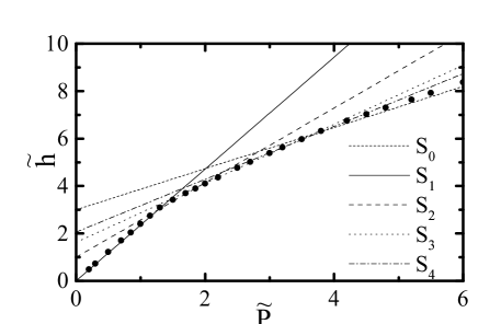
FIG. 12.: Ground state enthalpy per particle as a function of $\widetilde{P}$ from the simulations (black dots) and the analytical expression for the possible ordered structures. All points lie above at least one of the lines corresponding to the ordered structures.

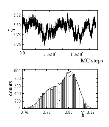
FIG. 13.: Time evolution of the enthalpy per particle for $\widetilde{P}=1.7,$ $T=0.0505,$ close to the fluid-quasicrystal transition. The histogram shows a clear double peak structure, with mean values compatible with those obtained from Fig. 10 for this temperature.

The numerical results are summarized in the phase diagram of Fig. 14. The sharp fluid-solid transition in the case of structures $S_{0}$ and $S_{1}$ are shown, as well as the corresponding to a quasicrystalline state. The error bars in these cases are taken as the width of the hysteresis loop in the enthalpy or the volume of the system. In addition, the approximate temperature where the system freezes in the other cases is also indicates, and in this case the error bars indicate the approximate temperature range in which the diffusion coefficient changes between 10 and 50 % of its value at high temperatures.

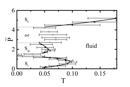
FIG. 14.: Pressure temperature phase diagram from the simulations (dsd stands for disordered). See text for more details.

We know from the results of the previous section that this phase diagram (particularly at intermediate pressures) is metastable at low temperatures. Since the numerical simulations are not able to reach the fundamental state in some cases, the determination of the equilibrium phase diagram at all values of $P$ and $T$ requires the direct comparison of the free energies of the structures found in the simulations and those known to be more stable in some cases (structures $S_{2},$ $S_{3}$, and $S_{4},$ for $\alpha=1.65$). The Gibbs free energy of the system can be obtained from the numerical simulations through the formula

$$\frac{G_{2}}{T_{2}}-\frac{G_{1}}{T_{1}}=\int_{1}^{2}\frac{V}{T}dP-\frac{H}{T^{2}}dT$$ (2)

where 1 and 2 stand for two set of values $P_{1}$, $T_{1}$ and $P_{2},$ $T_{2},$ and the integration is through an arbitrary (reversible) path in the $P$-$T$ plane joining points 1 and 2. This determines the free energy of those structures obtained in the numerical simulations up to an overall constant. Also the free energy of structures $S_{2},$ $S_{3},$ and $S_{4}$ may be determined in this way, by setting up the configuration of the system at zero temperature in these structures, and then performing a numerical simulation increasing temperature. After that, all that remains to be able to compare the free energies is to fix the additive constants. This was done by introducing in the model an additional external potential characterized by a strength $W$, with a periodicity chosen to favor the formation of the required structure. The reversible path from the ordered structure to that obtained in the simulation for a given point $P_{0},$ $T_{0}$ consisted of four steps: increasing $W$ from zero to some large value, increasing $T$ from $T_{0}$ to a large value, decreasing $W$ down to zero, and decreasing $T$ down to $T_{0}.$ The difference in Gibbs free energy $\Delta G$ between the two structures was calculated through this path by a generalization of the formula (2), given by

$$\Delta\left(G/T\right)|_{P_{0},T_{0}}=\oint\left(\frac{V}{T}dP+\frac{E_{W}}{TW}dW-\frac{H+E_{W}}{T^{2}}dT\right),$$ (3)

where $E_{W}$ is the potential energy of the particles in the artificial external potential, and $\oint$ indicates the integration along the above mentioned path. This was done three times with different external potential to fix all arbitrary constants between free energies of structures $S_{2},$ $S_{3},$ $S_{4},$ and the ones obtained in the simulations. After that, the free energies can be compared and the thermodynamical phase diagram constructed.

The complete thermodynamic phase diagram is shown in Fig. 15, where the stability region of each phase is shown. It is seen that the quasicrystalline state is in fact thermodynamically stable in a finite range of $P$ and $T,$ in spite of the value of $\alpha$ ($=1.65$), which is not the optimum value ($\alpha_{\text{qc}}\cong 1.618$) for the quasicrystalline structure. Only in the case $\alpha=\alpha_{\text{qc}}$ the quasicrystal is stable down to zero temperature, at the point $\widetilde{P}\equiv\widetilde{P}_{\text{qc}}\cong 1.7013$.

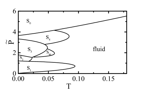
FIG. 15.: Complete pressure-temperature phase diagram for $\alpha=1.65.$ The errors in the limit of structures $S_{2}$, $S_{3}$, and $S_{4}$ are estimated to be $\pm 0.01$ in temperature. See text for discussions.

V Summary and discussion

In this paper I have discussed the phase behavior of a classical model of particles interacting through a particularly chosen isotropic potential. The interaction consists of a hard core plus a linear ramp potential, producing an effective greater size of the particles at low energies. The ground state of the system shows different periodic arrangements of the particles, depending on the values of $P$ and $\alpha$. There is a particular value of $P$ and $\alpha$ at which the ground state is a random quasicrystal. These periodic structures melt when temperature is increased through discontinuous phase transitions. In addition, at finite temperature, the quasicrystalline state is stabilized due to entropic effects.

It is usually believed that “…two-dimensional monoatomic systems interacting with central forces always form a triangular lattice.”[16] Although this is so for power laws and other kinds of interactions, the ground state configurations of our system show that this is not true in general. Even considering only crystalline ground states, there may be more than one atom per unit cell (2 for $S_{3}$ and 5 for $S_{4}$) and unequivalent sites within the structure (2 for $S_{4}$).

Having established the properties of the system for our model interaction, it is of basic importance to identify the conditions that an interaction potential must satisfy in order to obtain the kind of structures we got in our model. Although it is rather difficult to solve the problem in general, something can be said about. It is clear that the non-analyticity of the potential used is not a crucial element, actually, analytic potentials arbitrary close to the one used here may be easily constructed. First of all, let us analyze the necessary condition for the local stability of a triangular structure. Consider particles interacting through a potential $U\left(r\right),$ and distributed in a triangular lattice of lattice parameter $a$. At any lattice site the potential created by all other particles must have a minimum in order for the structure to be (locally) stable. The potential on that site (taken to be ${\bf r}=0$) created by a particle at a generic position ${\bf r}$ is, up to second order, of the form $U^{\prime\prime}\left(r\right)x^{2}+\frac{U^{\prime}\left(r\right)}{r}y^{2}+U^{\prime}\left(r\right)x+U\left(r\right)$, where $x$ ($y$) is the coordinate along (perpendicular to) ${\bf r}$. This potential must be summed up for all particles, and for lattices with rotational symmetry $C_{3}$ or higher it must reduce to a isotropic form. Considering the invariance of the trace of cuadratic forms under rotations, the cuadratic part $U_{2}\left(r\right)$ of the final effective potential can be written as

$$U_{2}\left(r\right)=\sum_{i=1}^{\infty}n_{i}\left[U^{\prime\prime}\left(d_{i}\right)+\frac{U^{\prime}\left(d_{i}\right)}{d_{i}}\right]d_{i}^{2},$$ (4)

where the sum is over all other particles, located at distances $d_{i}$ ($d_{1}=a$), and $n_{i}$ is the number of particles at those distances (for three dimensions the term containing $U^{\prime}$ gets an additional factor 2). The positiveness of this form is the condition for the stability of the lattice under small displacements of a single particle (global stability is more difficult to characterize), supposing the lattice parameter is fixed from outside. For $U\left(r\right)\sim 1/r^{\gamma}$ all terms of the sum in (4) are positive, and the structure is locally stable. For our potential, and analyzing a structure with lattice parameter $a$, $r_{1}>a>r_{0}$ , nearest neighbors have $U^{\prime\prime}\left(r\right)=0$ and $U^{\prime}\left(r\right)<0,$ and the structure is unstable. If the stability condition (4) is not satisfied for some lattice parameter $\widetilde{a}$, then it indicates at least the existence of an isostructural transition as a function of pressure between two triangular structures with lattice parameters $a_{0}<\widetilde{a}$ and $a_{1}>\widetilde{a}$. However, if first neighbors interaction dominate, it is easy to see that a $S_{2}$ kind of structure is more stable. In fact, consider two triangular structures with lattice parameters $a_{0}$ and $a_{1}$ which are degenerate at some pressure $P$. Their enthalpy per particle must be equal. This implies $-$if only first neighbors interaction is important$-$ that

$$Pa_{0}^{2}\sqrt{3}/2+3U(a_{0})=Pa_{1}^{2}\sqrt{3}/2+3U(a_{1}).$$ (5)

Now, the enthalpy of a $S_{2}$ structure with nearest neighbors distance $a_{0}$, and second neighbors distance $a_{1}$ is given by

$$Pa_{0}\sqrt{a_{1}^{2}-a_{0}^{2}/4}+U(a_{0})+2U(a_{1}),$$ (6)

and it is easy to see that this number is lower than the corresponding to the triangular structures. We conclude that stable structures other than the triangular one will occur if the condition

$$U^{\prime\prime}\left(r\right)+\frac{U^{\prime}\left(r\right)}{r}<0$$ (7)

is satisfied for some value of $r$. In cases where next-neighbors interactions cannot be neglected, a case by case analysis based on Eq. (4) is needed.

Our model does not contain an attractive part in the potential, and for this reason it lacks a liquid phase. However a liquid phase can be obtained within a generalized van der Waals approach,[17] in which an attractive interaction is included through an energy term proportional to $-v^{-1}$. In addition to the appearance of a liquid-gas coexistence line, this modification only renormalizes pressure, and does not affect the structure of the phases, nor the nature of the anomalies of the phase diagram that were discussed above.

The qualitative features of the phase diagram in the two-dimensional case have also been obtained in simulations with a three-dimensional system. The minimum value of $\alpha$ necessary to get the volume anomaly at melting is about $1.2$, both for two- and three-dimensional systems.

The results presented here might have importance in another context. The anomaly in the fluid-solid coexistence line, and the negative thermal expansion coefficient in this region remind strongly the same effects occurring in water. Actually, an interaction potential with a double minimum (which is related to the potential considered here) in one dimension has been analyzed recently, and has been suggested to be the origin of the density anomaly in water,[18] but this proposal has been questioned since it seems to give anomalous behaviors only in one dimension. [19] The results presented here show clearly that simple models with anomalous behavior may be constructed in two and three dimensions. A comparison of the phase diagrams of water with the corresponding to our system reveals in fact many coincidences, as the mentioned anomalies and the position of the different crystalline phases in the $P$-$T$ diagram, which occur near the pressure where the melting temperature is minimum. In addition, amorphous structures in ice are well known,[20] and the underlying mechanisms responsible for their formation may be related to those that originate our disordered structures when cooling down at intermediate pressures.

Finally, in order to get a better understanding of the dynamic and thermodynamic properties of the kind of system we dealt with, it would be interesting to find an experimental realization of an interaction potential satisfying condition (4). A colloidal system seems to be the natural candidate where to look for that realization.

VI Acknowledgments

The author thanks J. Simonín and J. Abriata for discussions. This work was financially supported by Consejo Nacional de Investigaciones Científicas y Técnicas (CONICET), Argentina.

REFERENCES

- [1] Electronic address: jagla@cab.cnea.edu.ar
- [2] W. B. Russel, D. A. Saville, and W. R. Schowalter, Colloidal Dispersions (Cambridge University Press, Cambridge, 1991), 2nd ed.
- [3] W. C. K. Poon and P. N. Pusey, in Observation, Prediction and Simulation of Phase Transitions in Complex Fluid, edited by M. Baus, L. F. Rull, and L. P. Ryckaert (Kluwer Academic Publishers, Dordrecht, 1994), pp. 3-44; D. H. Napper, Polymeric Stabilization of Colloidal Dispersions, (Academin Press, London, 1983), ch. 6.
- [4] P. Bolhuis and D. Frenkel, Phys. Rev. Lett. 72, 2211 (1994); P. Bolhuis, M. Hagen, and D. Frenkel, Phys. Rev. E 50, 4880 (1994); C. F. Tejero et al., Phys. Rev. Lett. 73, 752 (1994); ibid., Phys. Rev. E 51, 558 (1995).
- [5] P. C. Hemmer and G. Stell, Phys. Rev. Lett. 24,1284 (1970); Stell and P. C Hemmer, J. Chem. Phys. 56, 4274 (1972); J. M. Kincaid, G. Stell, and C. K. Hall, J. Chem. Phys. 65, 2161 (1976); J. M. Kincaid, G. Stell, and E. Goldmark, J. Chem. Phys. 65, 2172 (1976); J. M. Kincaid and G. Stell, J. Chem. Phys. 67, 420 (1977); J. M. Kincaid and G. Stell, Phys. Letters 65A, 131 (1978).
- [6] P. T. Cummings and G. Stell, Mol. Phys. 43,1267 (1981).
- [7] P. G. Bolhuis and D. Frenkel, J. Phys. Cond. Matter 9, 381 (1997).
- [8] C. Rascón et.al., J. Chem. Phys. 106, 6689 (1997).
- [9] In connection with this point see also P. G. Debenedetti, V. S. Raghavan, and S. S. Borick, J. Phys. Chem. 95, 4540 (1991).
- [10] B. J. Alder and T. E. Wainwright, Phys. Rev. 127, 359 (1962).
- [11] For a general reference on quasicrystals see C. Janot, Quasicrystals (Clarendon Press, Oxford, 1992).
- [12] C. Henley, J. Phys. A 21, 1649 (1988).
- [13] M. Widom, K. J. Strandburg, and R. H. Swendsen, Phys. Rev. Lett. 56, 706 (1987); K. J. Strandburg, Phys. Rev. B 60, 6071 (1989).
- [14] M. Widom, D. P. Peng, and C. L. Henley, Phys. Rev. Lett. 63, 310 (1989).
- [15] K. J. Strandburg, in Bond Orientational Order in Condensed Matter Systems, edited by K. Strandburg (Springer-Verlag, New York, 1992), ch. 2.
- [16] Reference 10, p. 60.
- [17] P. C. Hemmer and J. L. Lebowitz, in Phase Transitions and Critical Phenomena, Vol. 5b, Edited by C. Domb and M. S. Lebowitz (Academic Press, London, 1976).
- [18] C. H. Cho, S. Sing, and W. Robinson, Phys. Rev. Lett. 76, 1651 (1996).
- [19] E. Velasco, L. Mederos, and G. Navascués, Phys. Rev. Lett. 79, 179 (1997); C. H. Cho, S. Sing, and W. Robinson, Phys. Rev. Lett. 79, 180 (1997).
- [20] O. Mishima, L. D. Calvert, and E. Whalley, Nature 210, 393 (1984); P. Jenniskens and D. F. Blake, Science 265, 753 (1994).