PHYSICAL REVIEW B        VOLUME 56, NUMBER 17 1 NOVEMBER 1997-I, 11102$-$11118 Thermally activated resonant magnetization tunneling in molecular magnets:
Mn₁₂Ac and others

I Introduction

In recent years there has been great experimental and theoretical effort to observe and interpret quantum tunneling of magnetization in monodomain particles. The interest in this problem arises from the fact that the magnetization ${\bf M}$ of a particle containing a few thousand atoms is a macroscopic degree of freedom. Thus tunneling of the particle’s magnetization between different equilibrium orientations at low temperatures requires strong coherence between atomic spins and may be very sensitive to the interaction with the environment. A similar problem has been extensively studied in superconductors in the context of macroscopic quantum tunneling, where good agreement has been achieved between theory [1] and experiment. [2] Observation of magnetization tunneling is complicated by the difficulty in preparing identical magnetic particles. Experiments have been performed [3] on particles distributed over sizes and shapes. These experiments revealed temperature-independent magnetic relaxation which was attributed to tunneling. When an effort was made to narrow the distribution, resonance was observed [4, 5] in the absorption of the ac field, similar to the tunneling resonance in the ammonia molecule.

Difficulties in manufacturing identical magnetic particles for tunneling experiments have led to new techniques of measuring individual particles [6, 7] and to the idea of searching for magnetization tunneling in magnetic molecules of large spin. The system that caught the most recent attention is the crystal Mn₁₂ acetate (Mn₁₂Ac) having the chemical formula [Mn₁₂O₁₂(CH₃COO)₁₆(H₂O)₄]$\cdot$2CH₃COOH$\cdot$4H₂O. This compound has been synthesized by Lis,[8] but its physical properties had not received much attention until Sessoli et al. [9] noticed magnetic bistability of this system. In the Mn₁₂Ac molecule the 12 Mn ions are strongly bound ferrimagnetically via the superexchange through oxygen bridges. These molecules behave effectively as magnetic clusters of spin $S=10$, [9] as has been confirmed by the Curie-law temperature dependence of the susceptibility $\chi$. As follows from the very low value of the Curie constant, $\Theta_{C}\approx-0.05$ K, [10] the interaction between the Mn₁₂Ac molecules is very weak, presumably of the dipole-dipole origin. Mn₁₂Ac is characterized by a very strong uniaxial anisotropy ${\cal H}_{\rm A}=-DS_{z}^{2}$, where $D\simeq 0.72$ K from high-field EPR, [11] $D\simeq 0.75$ K from single-crystal magnetic susceptibility [12] measurements, and $D\simeq 0.77$ K from neutron scattering experiments. [13] This leads to a barrier of about $U=DS^{2}\simeq 75$ K between the states $\pm S$. Note, however, that experiments on resonant spin tunneling [14] (see below) suggest a value of $D$ close to 0.6 K and correspondingly the barrier height of 60 K.

The advantage of Mn₁₂Ac and other molecular magnets is that they are rather simple model systems, which facilitates their theoretical consideration and interpretation of experiments. Of course, it should be understood that a cluster of spin 10 cannot be treated macroscopically. The limit of macroscopic quantum tunneling is the one where the quantization of spin levels is irrelevant. On the contrary, in the Mn₁₂Ac cluster the distance between the ground-state and the first excited level is 12–15 K. At low temperature quantization of levels must, therefore, dominate the properties of the system. In this sense Mn₁₂Ac is closer to conventional quantum-mechanical systems where tunneling is of a resonant character. Nevertheless, as we shall see, the high value of spin leads to the macroscopic time scale for the dynamics of the magnetization, which has been tested in macroscopic experiments.

An important feature of Mn₁₂Ac is that if no strong transverse field is applied to the system, the interactions responsible for tunneling are small in comparison to the anisotropy energy ${\cal H}_{\rm A}=-DS_{z}^{2}$ which itself conserves the $S_{z}$ component of the spin. As a result of this and of the large spin of the system, the tunneling between low-lying energy levels should be extraordinary slow, which makes Mn₁₂Ac an excellent candidate for information storage at the molecular level. Another possible application of molecular magnets is that for quantum computing. For that application tunneling between the low-lying states should be made more pronounced, and the interaction with the environment destroying coherent oscillations of the spin between two wells should be kept small. This is hardly the case for Mn₁₂Ac where nuclear spins of manganese atoms strongly suppress the coherence. [15] The example of Mn₁₂Ac is, however, instructive since other systems with similar properties can be developed, which could be better candidates for quantum computation.

The first indications of magnetization tunneling in Mn₁₂Ac were seen in the magnetization relaxation experiments of Paulsen and Park [16] and the dynamic susceptibility measurements of Novak and Sessoli. [10] The measured relaxation rate of Mn₁₂Ac followed the Arrhenius law $\Gamma=\Gamma_{0}\exp(-U_{\rm eff}/T)$ with the peaks at some values of the longitudinal field $H_{z}$. These peaks were interpreted [10] as the resonant thermally assisted tunneling between the levels near the top of the barrier , which decreased the effective barrier height $U_{\rm eff}$. Subsequent dynamic hysteresis experiments [14] have proved that conjecture as they have shown many regularly spaced steps in the hysteresis loop at the values of $H_{z}$ at which the levels on both sides of the barrier come into resonance (see also Refs. [17, 18, 19, 20]). These steps indicate an increased relaxation rate at the corresponding bias fields $H_{z}$. Very recently a similar observation was made on Mn₁₂ phosphat [21] which was described as a magnetic cluster of spin $S=9.5$.

The transverse field $H_{x}$ applied to a uniaxial magnetic system mixes the unperturbed energy levels and enhances tunneling. The search for an increased tunneling in the transverse field has been undertaken in recent hysteresis [22] and dynamic susceptibility [23] measurements. The results show that the speeding up of the relaxation can be explained mostly through the classical effect of the barrier lowering in a transverse field, whereas the resonant tunneling peaks remaining after subtraction of this main effect are nearly independent of $H_{x}$. Actually both effects come from the same source: The classical height of the barrier can be determined quantum mechanically from the condition that the tunneling level splitting becomes comparable with the level spacing, which means strong nonresonant tunneling, i.e., the absense of a barrier at that level. [24]

A large number of experimental observations of magnetization tunneling in molecular magnets has been accumulated to date and the major relevant physical processes have been identified. A theoretical framework for the dynamical description of the combined process of the thermal activationand tunneling in these materials is still lacking, however. In particular, the form and the width of the tunneling peaks measured in experiments has not yet been explained. The aim of this article is to supply an appropriate theory.

The idea of the work is to apply the density matrix formalism in the case when the tunneling is caused by a transverse field $H_{x}$ which is small enough and can be considered as a perturbation. The applicability criterium of this method is $H_{x}\ll H_{\rm A}$, where $H_{\rm A}\equiv(2S-1)D/(g\mu_{B})$ is the anisotropy field. The latter in turn coincides with the critical value of the transverse field at which in the classical case of $S\gg 1$ the double-well structure of the spin energy disappears. For Mn₁₂Ac, the anisotropy field is of order 10 T, so that the condition $H_{x}\ll H_{\rm A}$ allows for rather large $H_{x}$. In this relevant range of the transverse field one can use the physically transparent and technically convenient basis of the eigenfunctions of the anisotropy energy ${\cal H}_{\rm A}=-DS_{z}^{2}$. The slow dynamics of the system driven by the thermal activation and tunneling processes can be described with the help of the adiabatic elimination of the fast degrees of freedom in the density matrix. The latter is a dynamical generalization of the calculation of the tunneling level splittings in the high orders of the perturbation theory. [25]

The remaining part of the paper is organized as follows. In Sec. II the properties of an isolated magnetic cluster in a transverse field are briefly reviewed and the perturbation theory is compared with other approaches to the problem. In Sec. III the density matrix equation (DME) for the uniaxial magnetic system interacting with a phonon bath is formulated and discussed. In Sec. IV the fast degrees of freedom in the DME are eliminated and a simplified system of equations describing the slow spin dynamics in terms of the diagonal and antidiagonal matrix elements connecting resonant pairs of levels in different wells is derived. It is shown that the level broadening due to the interaction with the environment suppresses coherent oscillations and, if strong enough, makes the motion of the spin between two degenerate levels overdamped. In this case, and also in the case of the thermally assisted quantum tunneling, when the relaxation rate is limited by the exponentially slow process of climbing up the energy barrier, the DME further simplifies to the system of kinetic balance equations for the level populations $N_{m}$ only. The latter describes the hopping of particles between adjaicent energy levels and through the barrier. In Sec. V the system of equations for the level populations $N_{m}$ is solved analytically in the Arrhenius regime $T\ll U\approx DS^{2}$. In Sec. VI the transition from the Arrhenius regime to pure quantum tunneling at lower temperatures is discussed. In Sec. VII the numerical results for the dependences of the escape rate on longitudinal and transverse fields in the Arrhenius regime are presented. Here we also analyze the influence of the Mn nuclear spins and a small scatter of the easy-axis directions in the oriented polycrystalls on resonant magnetization tunneling. In Sec. VIII further developments of the theory and suggestions for experiments are discussed.

II Tunneling level splitting and classical barrier lowering

The spin Hamiltonian of an isolated Mn₁₂Ac molecule in magnetic field ${\bf H}$ can be written in the form

$${\cal H}=-DS_{z}^{2}-H_{z}S_{z}-H_{x}S_{x},$$ (1)

where ${\bf H}$ stands for $g\mu_{B}{\bf H}$ with $g\simeq 1.9$. Henceforth we will usually drop the combination $g\mu_{B}$ for better readability of the formulas. The system is described by the $2S+1$ energy levels which in the absense of the transverse field $H_{x}$ are labeled by the spin projection $m$ on the $z$ axis and given by $\varepsilon_{m}=-Dm^{2}-H_{z}m$ (see Fig. 1). It can be easily checked that for the regularly spaced values of the longitudinal field $H_{z}$ satisfying

$$H_{z}=H_{zk}=kD,\qquad k=0,\pm 1,\pm 2,\ldots,$$ (2)

the energy levels on both sides of the barrier are pairwise degenerate

$$\varepsilon_{m}=\varepsilon_{m^{\prime}},\qquad m<0,\qquad m^{\prime}=-m-k.$$ (3)

\begin{picture}(11.0,10.5)\centerline{\hbox{\psfig{angle=0,width=284.52756pt}}} \end{picture}

FIG. 1.: Spin energy levels of a Mn₁₂Ac molecule for $H_{x}=0$ and $H_{z}=D$ corresponding to the first resonance, $k=1$, in Eq. (2).

The latest high-field EPR experiments [26] suggest that there are correction terms of the types $-AS_{z}^{4}$ and $-B(S_{+}^{4}+S_{-}^{4})$ in the spin Hamiltonian (1) of Mn₁₂Ac. This means that the degeneracy of different level pairs $m,m^{\prime}$ is actually achieved at slightly different values of $H_{z}$. We shall, however, ignore this effect in the following since it does not significantly change the results. As we shall see, only one or maximally two pairs of degenerate levels contribute to resonant tunneling, and hence the lack of simultaneous degeneracy of all appropriate level pairs is unimportant.

The model Hamiltonian (1) was a whetstone for different theories of spin tunneling long before its relevance for Mn₁₂Ac and other molecular magnets had been established. In the quasiclassical limit $S\gg 1$, the rate of tunneling from the ground-state for different values of $H_{z}$ was calculated by Chudnovsky and Gunther [27] with an exponential accuracy with the help of the instanton technique. Enz and Schilling [28] developed a more sophisticated version of the instanton approach to spins to obtain the ground-state tunneling level splitting with the prefactor. The latter result was rederived by Zaslavskii [29] by a more simple method based on the mapping onto a particle problem. Also, van Hemmen and Sütő [30, 31] formulated the WKB method for spin systems and calculated the tunneling rates and corresponding level splittings for the excited states of Eq. (1). Scharf, Wreszinski, and van Hemmen [32] proposed an approach based on a particle mapping with subsequent application of the WKB approximation to refine the results for the splittings of excited levels for systems with moderate spin. The applicability of this approach is confined, however, to the limit of small transverse fields $H_{x}$, where it is still possible to label the energy levels of Eq. (1) by the quantum number $m$.

In the case of small $H_{x}$, which, as we shall see, is relevant for magnetic clusters with moderate spin, the level splittings can be calculated in a more direct and simple way using the high-order perturbation theory. An early application of this method is due to Korenblit and Shender [33] who studied ground-state splitting in rare-earth compounds having high spin values (e.g., $S=8$ for Ho). Garanin [25] has derived a formula for the splitting of all levels of the Hamiltonian (1). A recent remake of the method is due to Hartmann-Boutron. [34] Schatzer, Breymann, and Thomas [35] extended the perturbative approach to describe tunneling in a system of two spins.

In the general biased case, the tunneling level splitting of the resonant level pair $m,m^{\prime}$ appears, minimally, in the $|m-m^{\prime}|$th order of a perturbation theory and is given by the shortest chain of matrix elements and energy denominators connecting the states $m$ and $m^{\prime}$,

$$\Delta\varepsilon_{mm^{\prime}}=2V_{m,m+1}\frac{1}{\varepsilon_{m+1}-\varepsilon_{m}}$$ (4)

$$\qquad\times V_{m+1,m+2}\frac{1}{\varepsilon_{m+2}-\varepsilon_{m}}\cdots V_{m^{\prime}-1,m^{\prime}},$$ (5)

where

$$V_{m,m+1}=\langle m|H_{x}S_{x}|m+1\rangle=\frac{1}{2}H_{x}l_{m,m+1},$$ (6)

$l_{m,m+1}\equiv\sqrt{S(S+1)-m(m+1)}$ are the matrix elements of the operator $S_{x}$, which are symmetric functions of their arguments, and $\varepsilon_{m}=-Dm^{2}-H_{z}m$ are the unperturbed energy levels. The calculation in Eq. (4) for the arbitrary resonance number $k$ yields the formula [24]

$$\Delta\varepsilon_{mm^{\prime}}=\frac{2D}{[(m^{\prime}-m-1)!]^{2}}$$ (7)

$$\qquad\times\sqrt{\frac{(S+m^{\prime})!(S-m)!}{(S-m^{\prime})!(S+m)!}}\left(\frac{H_{x}}{2D}\right)^{m^{\prime}-m},$$ (8)

which is the generalization of the zero-bias result of Ref. [25]. Note that here, according to the convention of Eq. (3), $m<0$, $m^{\prime}\equiv-m-k$, and hence $m^{\prime}-m>0$. Equation (4) describes the interaction between the pair of resonant levels $m,m^{\prime}$ through the intermediate levels in the virtual state. As is well known for the two-state problem, the splitting $\Delta\varepsilon_{mm^{\prime}}$ is exactly equal to the tunneling frequency $\Omega_{mm^{\prime}}$ with which the probability of finding the system in one of these states oscillates with time if the initial condition is an unperturbed eigenstate.

\begin{picture}(11.0,7.0)\centerline{\hbox{\psfig{angle=-90,width=341.43306pt}}} \end{picture}

FIG. 2.: Tunneling splittings $\Delta\varepsilon_{mm^{\prime}}$ for $H_{z}=0$ and different values of the transverse field. The results of Scharf, Wreszinski, and van Hemmen [32] are indiscernible from the perturbative ones in this scale and they are shown only for the one value of the transverse field.

The tunneling splittings given by Eq. (7) are represented in Fig. 2 for $H_{z}=0$ and different values of the transverse field, in comparison with the results of other approaches. One can see that the splittings change by orders of magnitude with changing $m$ by 1. If the splitting of the pair $m,m^{\prime}$ becomes comparable to the level spacing in the well, which is of order $2D|m|$, the tunneling becomes strong and of nonresonant character; i.e., the barrier for a particle going into the other well disappears. For this pair of levels the perturbation theory clearly breaks down, but for the next lower pair $m-1,m^{\prime}+1$ (see Fig. 1) it already works well.

The sharp boundary between the levels localized in one of the wells and the delocalized ones, which was observed above, is also characteristic for the classical theory where there is a similar separation between the localized and escape orbits at some energy. Accordingly, as was shown by Friedman, [36] the transverse-field dependence of the classical barrier height,

$$U(h_{x})=DS^{2}(1-h_{x})^{2},\qquad h_{x}\equiv\frac{H_{x}}{2SD},$$ (9)

can be reproduced for small $h_{x}$ with the help of the perturbative formula (7). Indeed, in the quasiclassical limit $1\ll|m|\ll S$ Eq. (7) for $H_{z}=0$ can be simplified to

$$\Delta\varepsilon_{mm^{\prime}}\cong\frac{2D|m|}{\pi}\left(\frac{H_{x}Se^{2}}{8Dm^{2}}\right)^{2|m|}$$ (10)

and compared to the level spacing $D|m|$ to obtain the value $m=m_{b}$ at which the barrier is effectively cut by the tunneling. For $|m|\gg 1$, the value of $m_{b}$ can be found with a good accuracy by equating the fraction in brackets in Eq. (10) to unity. The result has the form

$$m_{b}^{2}\cong 2S^{2}h_{x}\frac{e^{2}}{8},$$ (11)

which leads to the effective barrier height $U\cong DS^{2}-Dm_{b}^{2}\cong DS^{2}[1-2h_{x}(e^{2}/8)]$. This is in accordance with Eq. (9) for $h_{x}\ll 1$, except for the factor $e^{2}/8\approx 0.92$. The nontrivial feature of this derivation is that the resulting classical barrier lowering is of first order in $h_{x}$, although the corrections to the energy levels arise only in the second order of the perturbation theory. The latter have the form

$$\varepsilon_{m}^{(2)}=-Dm^{2}\left\{1+\frac{2S^{2}[S(S+1)+m^{2}]}{m^{2}[4m^{2}-1]}h_{x}^{2}\right\}.$$ (12)

It can be checked that for $m=m_{b}$ and $1\ll m_{b}\ll S$ the correction term in the curly brackets makes up the universal number $8/e^{4}\approx 0.15$. This means that near the renormalized top of the barrier , $m=m_{b}$, the perturbation theory relies on a small numerical parameter rather than on $h_{x}$. The artifact $e^{2}/8$ in Eq. (11) is the consequence of dropping the effect of the level mixing inside the wells described to lowest order by Eq. (12). It should be noted that $e^{2}/8$ also appears in the WKB results [30, 31, 32] for the tunneling level splitting in the case of small transverse field, and it can be attributed to the inaccuracy of the WKB method near the top of the barrier. In this article, we will neglect these effects and study the tunneling transitions between the wells perturbatively in the basis of the eigenstates of the operator $S_{z}$. It should be noted in addition that, as was checked by Chudnovsky and Friedman, [24] the level matching condition (2) remains uneffected by the transverse field at least up to fourth order in $h_{x}$.

Now let us consider the question how the level splitting changes from one level pair to another in more detail. For the pairs of resonant levels shown in Fig. 1, with the use of the basic formula (7) in the unbiased case, one comes to the result

$$\frac{\Delta\varepsilon_{m+1,m^{\prime}-1}}{\Delta\varepsilon_{mm^{\prime}}}=e^{4}\left(\frac{m}{m_{b}}\right)^{4}\frac{\left(1-\frac{1}{2|m|}\right)\left(1-\frac{1}{|m|}\right)}{\left(1+\frac{|m|}{S}\right)\left(1-\frac{|m|}{S}+\frac{1}{S}\right)},$$ (13)

where $m_{b}$ is given by Eq. (11). One striking implication of this formula is that the splitting ratio is large everywhere in the wells: Even near the top of the renormalized barrier, $m\sim m_{b}$, the tunneling splitting changes by a large factor $e^{4}\approx 55$, moving one step up the barrier. This universal behavior, independent of the spin value $S$ for $S\gg 1$, shows that even in the quasiclassical limit the tunneling splitting cannot be treated as a smooth function of the energy. The determination of the level at which the barrier disappears is, therefore, quite precise. Another consequence of Eq. (13) is that resonant tunneling is to the same extent inherent in models of large spin $S$ as in those of moderate spin.

III Spin-bath interactions and the density matrix equation

The thermally activated escape of the Mn₁₂Ac spin over the potential barrier $DS^{2}\simeq 70$ K is accompanied by the transitions between the energy levels with the energy differences ranging from $D(2S-1)\simeq 13$ K near the bottoms of the potential wells to $D\simeq 0.7$ K near the top of the barrier. Such a process requires an energy exchange between ${\bf S}$ and other degrees of freedom of the whole system.

The dipole-dipole interactions between different magnetic clusters contribute to the macroscopic magnetic induction ${\bf B}={\bf H}+4\pi{\bf M}$ which is actually “felt” by the spins and which should replace the external field H in all the formulas for spin tunneling and thermal activation. As was shown in dynamic hysteresis experiments, [14, 19] this internal field correction is quite essential for a careful analysis of the experimental data. The fluctuating part of the dipole-dipole interactions which could cause the spin relaxation has been shown to be inefficient by diluting the sample. [12] Indeed, this interaction is of the order of the dipole-dipole energy of two neighboring clusters, $E_{d}=(g\mu_{B}S)^{2}/v_{0}$, where $v_{0}$ is volume of the unit cell. Using $g=1.9$ and $v_{0}=(17.3{\rm\AA})^{2}\times 12.4{\rm\AA}$, [8] one obtains $E_{d}\simeq 0.06$ K [in accordance with the measured value of the Curie constant $\Theta_{C}=-0.05$ K (Ref. [10])] which is much smaller than the distances between the energy levels. There is also a more subtle argument, [37] based upon energy conservation and the nonequidistant character of the spin energy levels, which rules out the contribution of dipole-dipole interactions to the relaxation in the temperature range $T\ll U$.

The nuclear subsystem also cannot supply energies which would be large enough for the relaxation over the $70$ K barrier. Nevertheless, nuclear spins produce a hyperfine field on the effective electronic spin, which can give rise to tunneling. This mechanism will be considered in detail in Sec. VII. Here we will describe tunneling as caused by the externally applied transverse field $H_{x}$.

The remaining two types of the interaction of a Mn₁₂Ac spin with the environment are those with phonons and photons. Unlike the interactions reviewed above, the phonon and photon subsystems play the role of a thermal bath, rendering the spin subsystem a definite externally controlled temperature. It can be immediately seen that in the presense of phonons the photon processes can be safely neglected, since the light velocity $c$ is much greater than the sound velocity $v$ and, as a result, the photon density of states is smaller than the phonon one. At low temperatures the leading processes are the emission and absorption of phonons, accompanied by the hopping of spin between energy levels. At higher temperatures Raman scattering processes can become dominant. The energies of phonons in Mn₁₂Ac are large enough for the exchange with the spin subsystem: As follows from specific heat measurements, [10] the Debye temperature $\theta_{D}$ corresponding to the phonon energy at the edge of the Brillouin zone is about 36 K.

Spin-phonon interactions in materials with a strong crystal-field anisotropy are mainly due to the modulation of the crystal field by phonons. This mechanism was extensively studied in past years. [38] The possible spin-phonon coupling terms for substances of different symmetries are listed in Ref. [39]. For Mn₁₂Ac and other molecular magnets, the spin-phonon interactions, as well as the (presumably complicated) phonon modes themselves, have not yet been investigated. Moreover, an attempt to describe the interaction with phonons rigorously would lead to a serious complication of the formalism without bringing any new qualitative results. We will resort to various simplifications, assuming, in particular, that the phonon spectra of molecular magnets contain, as for an isotropic elastic body, one longitudinal and two transverse modes. Similar simplifications were also made in Ref. [37], where the pure thermal activation escape rate in Mn₁₂Ac was studied.

The lowest-order spin-phonon interactions allowed by the time-reversal symmetry are linear in phonon operators and bilinear in the spin operator components, containing various combinations $S^{\alpha}S^{\beta}$, where $\alpha,\beta=\pm,z$. The simplest of these interactions is due to the rotation of the anisotropy axis by transverse phonons. [40] We will use this mechanism for the illustration of our method since it does not employ any unknown characteristics of the crystal-field distortions accompanying other types of lattice vibrations.

For the arbitrarily oriented anisotropy axis n, the anisotropy part of the spin Hamiltonian (1) can be written as ${\cal H}_{A}=-D({\bf nS})^{2}$. Transverse phonons change the vector n by $\delta{\bf n}=[\delta\mathchoice{{\hbox{\boldmath$\displaystyle\phi$}}}{{\hbox{\boldmath$\textstyle\phi$}}}{{\hbox{\boldmath$\scriptstyle\phi$}}}{{\hbox{\boldmath$\scriptscriptstyle\phi$}}}\times{\bf n}]$, where $\delta\mathchoice{{\hbox{\boldmath$\displaystyle\phi$}}}{{\hbox{\boldmath$\textstyle\phi$}}}{{\hbox{\boldmath$\scriptstyle\phi$}}}{{\hbox{\boldmath$\scriptscriptstyle\phi$}}}=(1/2)\nabla\times{\bf u}$ is the local rotation of the lattice and u is the lattice displacement. The first order term on $\delta{\bf n}$ in ${\cal H}_{A}$ gives the spin-phonon Hamiltonian which in coordinate form reads

$${\cal H}_{\rm sp}=D\{S_{z},S_{x}\}\omega_{zx}+D\{S_{z},S_{y}\}\omega_{zy},$$ (14)

where

$$\omega_{\alpha\beta}\equiv\frac{1}{2}\left(\frac{\partial u_{\alpha}}{\partial r_{\beta}}-\frac{\partial u_{\beta}}{\partial r_{\alpha}}\right),$$ (15)

and $\{S_{\alpha},S_{\beta}\}$ is the anticommutator. In terms of phonon operators $a_{k\lambda}$ and $a_{k\lambda}^{\dagger}$,

$${\bf u}=\frac{i}{(2MN)^{1/2}}\sum_{{\bf k}\lambda}\frac{{\bf e}_{{\bf k}\lambda}e^{i{\bf kr}}}{(\omega_{k\lambda})^{1/2}}(a_{k\lambda}-a_{k\lambda}^{\dagger}),$$ (16)

where $M$ is the unit cell mass, $N$ is the number of cells in the lattice, ${\bf e}_{{\bf k}\lambda}$ is the phonon polarization vector, $\lambda=t,t,l$ is the polarization, and $\omega_{k\lambda}=v_{\lambda}k$ is the phonon frequency. Performing differentiation in Eq. (15), one can transform Eq. (14) to

$${\cal H}_{\rm sp}=-\frac{1}{N^{1/2}}\sum_{{\bf k}\lambda}V_{k}\{S_{z},(\mathchoice{{\hbox{\boldmath$\displaystyle\eta$}}}{{\hbox{\boldmath$\textstyle\eta$}}}{{\hbox{\boldmath$\scriptstyle\eta$}}}{{\hbox{\boldmath$\scriptscriptstyle\eta$}}}_{{\bf k}\lambda}{\bf S})\}(a_{k\lambda}-a_{k\lambda}^{\dagger}).$$ (17)

Here the spin-phonon amplitide $V_{k}$ is given by

$$V_{k}=\frac{D}{2^{3/2}}\left(\frac{\omega_{k\rm t}}{\Omega_{t}}\right)^{1/2},\qquad\Omega_{t}\equiv Mv_{t}^{2},$$ (18)

and the vector $\mathchoice{{\hbox{\boldmath$\displaystyle\eta$}}}{{\hbox{\boldmath$\textstyle\eta$}}}{{\hbox{\boldmath$\scriptstyle\eta$}}}{{\hbox{\boldmath$\scriptscriptstyle\eta$}}}_{{\bf k}\lambda}$ is determined by

$$\eta_{{\bf k}\lambda}^{z}=0,\qquad\eta_{{\bf k}\lambda}^{x,y}=e_{{\bf k}\lambda}^{z}n_{\bf k}^{x,y}-e_{{\bf k}\lambda}^{x,y}n_{\bf k}^{z},$$ (19)

where ${\bf n}_{\bf k}\equiv{\bf k}/k$. On can see that the coupling to longitudinal phonons in Eq. (17) vanishes, as it should be, since ${\bf e}_{{\bf k}\rm l}={\bf n}_{\bf k}$.

The evolution of a spin system coupled to an equilibrium heat bath can be described by the density matrix equation. The diagonal elements of the density matrix, $\rho_{mm}\equiv N_{m}$, describe the population of the energy levels. In the absense of interactions noncommuting with $S_{z}$ in the spin Hamiltonian $\cal H$, the DME reduces to the closed system of kinetic balance equations, or master equations, for the populations $N_{m}$ in the basis of the eigenstates of the operator $S_{z}$. The latter was applied to describe the thermoactivation process in uniaxial spin systems, as Mn₁₂Ac, in Refs. [37] and [42]. If a transverse field or another level mixing perturbation is applied to the system, the nondiagonal elements of the DME appear, whose slow dynamics describes the tunneling process. The major advantage of the DME is that it provides a natural account of resonant tunneling in systems of moderate spin, which is lost in quasiclassical approaches for truly macroscopic systems.

A common routine for obtaining a system of kinetic balance equations is to calculate the transition probabilities according the Fermi golden rule and then insert them into the equations that are themselves postulated but not derived. Such an approach is methodically insufficient since the transition probabilities are obtained with the help of the time dependent perturbation theory where the probability of finding the system in states differing from the initial fully occupied state are used as a small parameter. In other words, this method describes only the initial stage of the relaxation process for a special type of initial conditions. Although it incidently leads to the correct master equation, the same is not true for the general DME. Indeed, spin-phonon couplings of the type $\sum_{k}\Psi_{k}S_{z}^{2}a_{k}a_{k}^{\dagger}$, corresponding to the elastic scattering of phonons, do not result in transitions between the energy levels and do not contribute to the coefficients of the master equation. On the other hand, such terms modulate the energy levels and contribute to the linewidths, which manifest themselves in the dynamics of the nondiagonal elements of the density matrix.

A rigorous method of the derivation of the density matrix equation valid for all times employs the projection operator technique. [43, 44, 45, 46] For spin systems, the details of calculations are described in Ref. [47]. The resulting DME can be found in Ref. [48], where the model without single-site anisotropy, accounting for both one-phonon and Raman scattering processes, was used to derive the Landau-Lifshitz-Bloch equation for ferromagnets. This DME is written in terms of the Hubbard operators $X^{mn}\equiv|m\rangle\langle n|$ forming the complete basis for the spin subsystem. In the Heisenberg representation the operators $X^{mn}$ are related to the spin density matrix: $\rho_{mn}=\langle X^{mn}(t)\rangle$. For the present model described by Eqs. (1) and (17), the resulting DME reads

$$\dot{X}^{mn}=i\omega_{mn}X^{mn}-\frac{i}{2}H_{x}(l_{m,m+1}X^{m+1,n}+l_{m,m-1}X^{m-1,n}$$ (20)

$$\qquad-l_{n,n+1}X^{m,n+1}-l_{n,n-1}X^{m,n-1})+R_{mn},$$ (21)

where $\omega_{mn}\equiv\varepsilon_{m}-\varepsilon_{n}$ are the frequencies associated with the transition $n\to m$, the unperturbed energy levels $\varepsilon_{m}$ are given by $\varepsilon_{m}=-Dm^{2}-H_{z}m$, the factors $g\mu_{B}$ and $\hbar$ are dropped for convenience, the matrix elements $l_{m,m\pm 1}$ are given by Eq. (6), and $R_{mn}$ is the relaxation term. The latter has the non-Markovian form

$$R_{mn}=-\int_{t_{0}}^{t}dt^{\prime}\frac{1}{N}\sum_{{\bf k}\lambda}V_{k}^{2}\{Af_{k}(t^{\prime}-t)-Bf_{k}(t-t^{\prime})\},$$ (22)

where

$$A=Q_{S}(t^{\prime})[Q_{S}(t),X^{mn}(t)],$$ (23)

$$B=[Q_{S}(t),X^{mn}(t)]Q_{S}(t^{\prime}),$$ (24)

the spin operator combination $Q_{S}\equiv\{S_{z},(\mathchoice{{\hbox{\boldmath$\displaystyle\eta$}}}{{\hbox{\boldmath$\textstyle\eta$}}}{{\hbox{\boldmath$\scriptstyle\eta$}}}{{\hbox{\boldmath$\scriptscriptstyle\eta$}}}_{{\bf k}\lambda}{\bf S})\}$ comes from the spin-phonon Hamiltonian (17), the function $f_{k}(\tau)$ characterizing the bath in the present case of the one-phonon processes is given by

$$f_{k}(\tau)=n_{k}e^{i\omega_{k}\tau}+(n_{k}+1)e^{-i\omega_{k}\tau},$$ (25)

$n_{k}\equiv(e^{\omega_{k}/T}-1)^{-1}$ are the boson occupation numbers, and $\omega_{k}\equiv\omega_{kt}$ are the frequencies of transverse phonons.

In Eq. (23) the spin operators should be expanded over the $X^{mn}$ basis as follows:

$$S_{+}=\sum_{m=-S}^{S-1}l_{m,m+1}X^{m+1,m},\qquad S_{z}=\sum_{m=-S}^{S}mX^{mm},$$ (27)

$$S_{-}=\sum_{m=-S}^{S-1}l_{m,m+1}X^{m,m+1},\qquad S_{\pm}\equiv S_{x}\pm iS_{y}.$$

For the one-phonon processes, the integral over $t^{\prime}$ in Eq. (22) converges on the scale of $1/\omega_{mn}$ which is much shorter than the relaxation time of the spin system. Hence, the lower limit of this integral can be extended to $t_{0}=-\infty$ and the $t^{\prime}$ dependences of the operators $X^{mn}$ in the relaxation term can be considered as governed solely by the conservative part of the DME (20). Finding these time dependences is a matter of numerical work, if the transverse field $H_{x}$ is not small. Here serious complications arise, since the evolution of each operator $X^{mn}$ is a linear combination of all possible types of spin motion. This means simply that the unperturbed basis we have chosen is not suitable in situations with strong level mixing. However, in the case of small $H_{x}$ one can neglect these effects and use the unperturbed time dependences

$$X^{mn}(t^{\prime})=e^{i\omega_{mn}(t^{\prime}-t)}X^{mn}(t).$$ (28)

Now one can calculate combinations $A$ and $B$ in Eq. (23) with the use of the representations (27) and the equal-time relation $X^{mk}X^{ln}=X^{mn}\delta_{kl}$ which replaces the commutation relations for the spin components. The sum over the phonon polarizations $\lambda$ in Eq. (22) can be done using Eq. (19) and the property of the polarization vectors $\sum_{\lambda}e_{\lambda}^{\alpha}e_{\lambda}^{\beta}=\delta_{\alpha\beta}$. Neglecting the imaginary part of the relaxation term $R_{mn}$, corresponding to the renormalization of the spin energy levels due to the coupling to the bath, one arrives at the final form of $R_{mn}$:

$$R_{mn}=\frac{1}{2}\bar{l}_{m,m+1}\bar{l}_{n,n+1}[W_{m,m+1}+W_{n,n+1}]X^{m+1,n+1}$$ (29)

$$\qquad{}-\frac{1}{2}[\bar{l}_{m,m+1}^{2}W_{m+1,m}+\bar{l}_{n,n+1}^{2}W_{n+1,n}]X^{mn}$$ (30)

$$\qquad{}+\frac{1}{2}\bar{l}_{m,m-1}\bar{l}_{n,n-1}[W_{m,m-1}+W_{n,n-1}]X^{m-1,n-1}$$ (31)

$$\qquad{}-\frac{1}{2}[\bar{l}_{m,m-1}^{2}W_{m-1,m}+\bar{l}_{n,n-1}^{2}W_{n-1,n}]X^{mn}.$$ (32)

Here $\bar{l}_{m,m\pm 1}\equiv l_{m,m\pm 1}(2m\pm 1)$ with the factor $2m\pm 1$ coming from the operator $S_{z}$ in Eq. (17), and the universal rate constant $W_{mn}=W(\omega_{mn})$ of the one-phonon processes is given by

$$W(\omega)=\frac{2}{3}v_{0}\!\!\int\!\!\frac{d{\bf k}}{(2\pi)^{3}}V_{k}^{2}\big{\{}(n_{k}+1)\pi\delta(\omega_{k}+\omega)$$ (33)

$$\qquad\qquad\qquad\qquad{}+n_{k}\pi\delta(\omega_{k}-\omega)\big{\}},$$ (34)

where $v_{0}$ is the unit cell volume and the overall factor 2/3 says that only two transverse modes of the total three phonon modes are active in the relaxation mechanism under consideration. One can check that the rate constant satisfies the detailed balance condition $W(\omega)=W(-\omega)\exp(-\omega/T)$. At low temperatures phonons die out and $W(\omega)$ with $\omega>0$, which corresponds to the absorption of a phonon, becomes exponentially small. The result for $W(\omega)$ with $\omega<0$ (the emission of a phonon) calculated with the help of Eqs. (33) and (18) reads

$$W=\frac{D^{2}|\omega|^{3}}{24\pi\Theta^{4}}(n_{|\omega|}+1)\propto\left\{\begin{array}[]{ll}\omega^{2}T,&|\omega|\ll T\\ |\omega|^{3},&T\ll|\omega|\end{array}\right.$$ (35)

(cf. Ref. [49]). Here we have used $\theta_{D}^{3}=(\hbar v_{t})^{3}/v_{0}$ for the Debye temperature $\theta_{D}\sim\hbar\omega_{k_{\rm max}}$. The constant $\Theta$ is defined as $\Theta^{4}\equiv\Omega_{t}\theta_{D}^{3}=\hbar^{3}\rho^{2}v_{t}^{5}$, where $\rho$ is the density and $\Omega_{t}$ is given by Eq. (18).

Note that Eq. (20) with $R_{mn}$ given by Eq. (29) is still an operator equation, and the equation of motion for the density matrix elements, $\rho_{mn}\equiv\langle X^{mn}\rangle$, should be obtained by taking its quantum-statistical average over the initial state of the spin. This is, however, a trivial task, since the equation for $X^{mn}$ is linear.

In the case $H_{x}=0$ the density matrix equation (20) and (29) reduces to a system of kinetic balance equations for the diagonal elements $N_{m}\equiv X^{mm}$, the equilibrium solution of which is given by

$$N_{m}^{(0)}=\frac{1}{Z}e^{-\varepsilon_{m}/T},\qquad Z=\!\!\sum_{m=-S}^{S}\!\!e^{-\varepsilon_{m}/T}.$$ (36)

The thermoactivation relaxation rate $\Gamma$ in the model with $H_{x}=0$ was studied in Ref. [37] and recently in Ref. [42]. In the latter work Raman scattering processes have also been taken into account, and the spin relaxation rate was calculated for arbitrary ratios $U/T$ in terms of the integral relaxation time $\tau_{\rm int}$. It was shown that in systems with larger spin values, even in the Arrhenius regime $U/T\gg 1$, there are several limiting cases for the prefactor $\Gamma_{0}$ in the expression $\Gamma=\Gamma_{0}\exp(-U/T)$ as a result of the interplay between the one-phonon and Raman scattering processes. Here we concentrate on the low-temperature region, and thus only one-phonon processes will be considered.

IV Slow dynamics of the density matrix: coherence and tunneling between resonant levels

The possible frequencies, with which the density matrix elements $X^{mn}$ evolve in time according to the DME (20), range from $\omega_{0S}=DS^{2}$ (for $H_{z}=0$) to very small ones corresponding to overbarrier relaxation and tunneling. In the low-temperature range $T\ll U$, these fast motions decay with the rate corresponding to the relaxation inside one well, which is much larger than the thermoactivation escape rate or the tunneling rates. In the long-time or low-frequency dynamics, the variables $X^{mn}$ corresponding to the large $\omega_{mn}$ play the role of “slave” degrees of freedom, adjusting themselves to the evolution of the slow variables, and hence they can be adiabatically eliminated.

The slow variables of our problem are the diagonal matrix elements $N_{m}=X^{mm}$, as well as the antidiagonal elements $X^{mm^{\prime}}$ whose transition frequency $\omega_{mm^{\prime}}\equiv\varepsilon_{m}-\varepsilon_{m^{\prime}}$ is the detuning of the resonant levels $m$ and $m^{\prime}$

$$\omega_{mm^{\prime}}=(H-H_{k})(m^{\prime}-m)$$ (37)

[cf. Eqs. (2) and (3)]. The equations of motion for these slow variables can be obtained in the following way. In Eq. (20) for $X^{mm}$, the terms containing $X^{m+1,m}$ and $X^{m,m+1}$, which are generated minimally by nonzero $X^{m^{\prime}m}$ and $X^{mm^{\prime}}$, correspondingly, are responsible for tunneling in the lowest approximation. In the dynamical equations for these elements one can neglect the terms $\dot{X}^{m+1,m}$ and $\dot{X}^{m,m+1}$, as well as the relaxation terms, since the frequencies $\omega_{m+1,m}$ and $\omega_{m,m+1}$ are large on the scale of relaxational and tunneling processes. Then, in the case of $X^{m+1,m}$, this element can be expressed with the help of its dynamical equation through $X^{m+2,m}$ as

$$X^{m+1,m}=\frac{\frac{1}{2}H_{x}l_{m,m+1}}{\omega_{m+1,m}}X^{m+2,m}.$$ (38)

In the right part of this equation the terms containing $X^{mm}$, $X^{m+1,m+1}$, and $X^{m+1,m-1}$ have been dropped because retaining them would be against our strategy of going across the barrier along the shortest path to $X^{m^{\prime}m}$. For the same reason we have also dropped the terms $X^{m-1,m}$ and $X^{m,m-1}$ in the equation for $X^{mm}$. Retaining all these terms would imply taking into account the level mixing inside the wells, which we neglect for small transverse fields. Now, Eq. (38) can be iterated until $X^{m+1,m}$ is expressed through $X^{m^{\prime}m}$, and similar can be performed on $X^{m,m+1}$. Substituting their expressions into the equation for $X^{mm}$, one arrives at the slow equation

$$\dot{X}^{mm}=\frac{i}{2}\Omega_{mm^{\prime}}(X^{mm^{\prime}}-X^{m^{\prime}m})+R_{mm},$$ (39)

where $\Omega_{mm^{\prime}}$ is the tunneling frequency coinciding with the tunneling level splitting $\Delta\varepsilon_{mm^{\prime}}$ of Eq. (7). One can see now that the algorithm used here for the adiabatic elimination of the fast degrees of freedom in the density matrix equation is the dynamic counterpart of the perturbative approach leading to the chain formula (4). The antidiagonal matrix elements $X^{mm^{\prime}}$ and $X^{m^{\prime}m}$ are generated, in turn, by the diagonal elements $X^{mm}$ and $X^{m^{\prime}m^{\prime}}$, and the dynamical equations for them can be obtained in a similar way. The result for $X^{mm^{\prime}}$ reads

$$\dot{X}^{mm^{\prime}}=i\omega_{mm^{\prime}}X^{mm^{\prime}}-\frac{i}{2}\Omega_{mm^{\prime}}(X^{m^{\prime}m^{\prime}}-X^{mm})+R_{mm^{\prime}}.$$ (40)

For the matrix elements $X^{m^{\prime}m^{\prime}}$ and $X^{m^{\prime}m}$ one obtains equations similar to Eqs. (39) and (40).

To formulate the resulting system of slow equations in a more convenient form, we introduce

$$Z_{mm^{\prime}}\equiv N_{m^{\prime}}-N_{m},$$ (41)

$$Y_{mm^{\prime}}\equiv i(X^{mm^{\prime}}-X^{m^{\prime}m}),$$ (42)

$$X_{mm^{\prime}}\equiv X^{mm^{\prime}}+X^{m^{\prime}m}.$$ (43)

These variables satisfy the system of equations

$$\dot{N}_{m}=\frac{1}{2}\Omega_{mm^{\prime}}Y_{mm^{\prime}}+R_{mm},$$ (44)

$$\dot{N}_{m^{\prime}}=-\frac{1}{2}\Omega_{mm^{\prime}}Y_{mm^{\prime}}+R_{m^{\prime}m^{\prime}}$$ (45)

[cf. Eq. (39)] and

$$\dot{Z}_{mm^{\prime}}=-\Omega_{mm^{\prime}}Y_{mm^{\prime}}+R_{m^{\prime}m^{\prime}}-R_{mm},$$ (46)

$$\dot{Y}_{mm^{\prime}}=\Omega_{mm^{\prime}}Z_{mm^{\prime}}-\omega_{mm^{\prime}}X_{mm^{\prime}}-\Gamma_{mm^{\prime}}Y_{mm^{\prime}},$$ (47)

$$\dot{X}_{mm^{\prime}}=\omega_{mm^{\prime}}Y_{mm^{\prime}}-\Gamma_{mm^{\prime}}X_{mm^{\prime}},$$ (48)

where the equation first of Eqs. (46) is a consequence of Eqs. (44). The conservative part of Eqs. (46) describes the precession of the pseudospin $\mathchoice{{\hbox{\boldmath$\displaystyle\sigma$}}}{{\hbox{\boldmath$\textstyle\sigma$}}}{{\hbox{\boldmath$\scriptstyle\sigma$}}}{{\hbox{\boldmath$\scriptscriptstyle\sigma$}}}_{mm^{\prime}}\equiv\{X_{mm^{\prime}},Y_{mm^{\prime}},Z_{mm^{\prime}}\}$ in the pseudofield ${\bf H}_{mm^{\prime}}\equiv\{\Omega_{mm^{\prime}},0,\omega_{mm^{\prime}}\}$. In the absense of dissipation, in resonance ($\omega_{mm^{\prime}}=0$), the pseudospin rotates in the $y,z$ plane, and the difference of the level populations $Z_{mm^{\prime}}$ oscillates with time. Note, however, that the $Y$ and $X$ components of the pseudospin have nothing to do with the actual spin components $S_{y}$ and $S_{x}$ which remain zero, see Eq. (27). The only exclusion is the resonance between the two neighboring levels $m$ and $m+1$ near the top of the barrier , which is realized, e.g., for $S$ odd and $H_{z}=0$. In this case, which is actually no longer the tunneling case since $\Omega_{m,m+1}\propto H_{x}$ is not suppressed by the anisotropy, the rotation of the pseudospin couples to the rotation of the real spin.

Since the tunneling frequency $\Omega_{mm^{\prime}}$ is typically very small, the correspondingly small detuning $\omega_{mm^{\prime}}\geq\Omega_{mm^{\prime}}$ [see Eq. (37)] is sufficient to suppress the resonance. On the other hand, a small ac field $H_{z}(t)$ with a frequency about $\Omega_{mm^{\prime}}$ giving rise to the corresponding $z$ component of the pseudofield $\omega_{mm^{\prime}}(t)$ [see Eq. (37)] can excite the tunneling resonance. The latter, however, can only happen under two rather severe conditions:

$$H_{z}(t)\ll\frac{\hbar\Omega_{mm^{\prime}}}{(m^{\prime}-m)},\qquad T\ll\hbar\Omega_{mm^{\prime}}.$$ (49)

The former is the condition of the linear resonance, whereas the latter requires that the pseudospin have a strong preference along the $x$ axis, in other words, that only the lower of the tunneling-splitted states (the even one) is thermally populated. The temperatures required by the second condition are so small that only the resonance between the ground-state levels $m=\pm S$ can be discussed.

The small value of the pseudofield $\Omega_{mm^{\prime}}$ in resonant tunneling equations (46) suggests an important role of the relaxation terms. The diagonal relaxation term $R_{mm}$ following from Eq. (29) has the form

$$R_{mm}=\bar{l}_{m,m+1}^{2}(W_{m,m+1}N_{m+1}-W_{m+1,m}N_{m})$$ (50)

$$\qquad{}+\bar{l}_{m,m-1}^{2}(W_{m,m-1}N_{m-1}-W_{m-1,m}N_{m}),$$ (51)

describing the exchange of particles with the levels $m\pm 1$. For the antidiagonal matrix elements, the relaxation term $R_{mm^{\prime}}$ in Eq. (29) contains $X^{mm^{\prime}}$ itself, as well as the matrix elements $X^{m\pm 1,m^{\prime}\pm 1}$. These matrix elements do not belong, however, to the antidiagonal ones (see Fig. 1); they are small slave variables that have been eliminated above. Dropping them leads to

$$\Gamma_{mm^{\prime}}=\Gamma_{m}+\Gamma_{m^{\prime}},$$ (52)

$$\Gamma_{m}=\frac{1}{2}(\bar{l}_{m,m+1}^{2}W_{m+1,m}+\bar{l}_{m,m-1}^{2}W_{m-1,m}).$$ (53)

Here the terms $\Gamma_{m}$ and the analogous $\Gamma_{m^{\prime}}$ are the linewidths of the levels $m$ and $m^{\prime}$ arising from the transitions to the levels $m\pm 1$ and $m^{\prime}\pm 1$ with the absorption or emission of an energy quantum.

At temperatures $T\ll\omega_{\rm A}=(2S-1)D$, which is about 13 K for Mn₁₂Ac, most of the particles are in the ground states $m=\pm S$. The linewidths of these states are much smaller than that of excited ones since in Eq. (52) the emission term is absent and the absorption term is small as $\exp(-\omega_{\rm A}/T)$. Further lowering of the temperature leads to the suppression of the thermoactivation relaxation mechanism and, simultaneously, to the vanishing of dissipation in the ground state. Thus, the spin of the magnetic cluster behaves like an undamped two-level system (TLS). It is, however, well known (see, e.g., Ref. [50]) that the coupling of the TLS to the bath strongly changes its dynamics, and one can ask where this coupling was lost in our calculations. The answer is that treating the non-Markovian relaxation term (22) we have used the simplest unperturbed $t^{\prime}$ dependences (28) for the spin operators of Eqs. (23) and (27), which do not describe the tunneling motion. This tunneling motion couples, however, to a very small number of extremely-long-wavelength phonons, and their contribution to the relaxation terms is smaller by a factor of order $(\Omega_{-S,S}/\omega_{\rm A})^{3}\exp(\omega_{\rm A}/T)$ [see Eq. (35)] than that of the regular phonon processes. Thus, the coupling of the tunneling mode to the bath becomes important only at very low temperatures. In this range serious complications arise (see, e.g., Ref. [50]) since the pseudospin part of the effective TLS Hamiltonian, ${\cal H}_{\rm TLS}=-\mathchoice{{\hbox{\boldmath$\displaystyle\sigma\Omega$}}}{{\hbox{\boldmath$\textstyle\sigma\Omega$}}}{{\hbox{\boldmath$\scriptstyle\sigma\Omega$}}}{{\hbox{\boldmath$\scriptscriptstyle\sigma\Omega$}}}$, is no longer large in comparison to the coupling to the bath and the perturbation theory breaks down.

The equation of motion for the pseudospin, Eq. (46), is not closed because the relaxation term in the first line couples it to other levels. If we neglect this coupling for a moment, then the eigenvalues $\lambda$ of Eq. (46) determined as $X,Y,Z\propto e^{-\lambda t}$ are given by the roots of the cubic equation $(\lambda-\Gamma)^{2}\lambda+\Omega^{2}(\lambda-\Gamma)+\omega^{2}\lambda=0$, where we have dropped the index $mm^{\prime}$. This equation can be solved only in limiting cases. In particular, in resonance ($\omega=0$) the last equation of Eqs. (46) decouples from the first two ones, which describe now a damped harmonic oscillator with $\lambda_{1,2}=(1/2)(\Gamma\pm\sqrt{\Gamma^{2}-4\Omega^{2}})$. One can see that the tunneling oscillations of the particle between the two levels become overdamped for $\Gamma>2\Omega$. In the small damping case, the solution of Eq. (46) with the initial condition $Z(0)=1$ has an interesting two-scale-relaxation form

$$Z(t)=\frac{\Omega^{2}}{\Omega^{2}+\omega^{2}}\exp\left(-\frac{\Omega^{2}/2+\omega^{2}}{\Omega^{2}+\omega^{2}}\Gamma t\right)\cos(\sqrt{\Omega^{2}+\omega^{2}}t)$$ (54)

$${}+\frac{\omega^{2}}{\Omega^{2}+\omega^{2}}\exp\left(-\frac{\Omega^{2}}{\Omega^{2}+\omega^{2}}\Gamma t\right).$$ (55)

These results should not be overstated for the present model because in the underdamped case the neglected relaxation terms in the equation for $Z$ can be of the same order of magnitude as the accounted ones in the equations for $X$ and $Y$. In this case the pseudospin concept breaks down and one should use the two equations (44) instead of the first equation of Eqs. (46). But in the case of strong damping the level populations cannot deviate substantially from their equilibrium values because of the slow tunneling motion, and the different terms in the diagonal relaxation terms $R_{mm}$ given by Eq. (50) nearly cancel each other. Here the concept of the independent pseudospin is justified, and one can see that its motion is indeed overdamped. Neglecting the terms $\dot{X}$ and $\dot{Y}$ in Eqs. (46), one eliminates $X$ and $Y$ and comes to the simple relaxational equation for $Z$ with $\lambda=\Omega^{2}\Gamma/(\omega^{2}+\Gamma^{2})$.

The argument in favor of the pseudospin model is that there can be other relaxation mechanisms, such as those due to spin-spin interactions, which contribute only to the linewidths (i.e., to the transverse relaxation rate) and not to the transition probabilities (i.e., to the longitudinal relaxation rate). In this typical for the magnetic resonance situation the term $R_{m^{\prime}m^{\prime}}-R_{mm}$ in the first equation of Eqs. (46) can be neglected on the relatively short scale of the transverse relaxation time. In our model the dipole-dipole interactions could play such a role, but for Mn₁₂Ac the main effect of such a type comes from nuclear spins (see Sec. VII).

The possibility of the overdamping of the coherent spin oscillations was pointed out by Garg, [51] who considered resonant tunneling with the help of a phenomenological damped Schrödinger equation in the matrix representation in the unperturbed basis. Although the qualitative conclusions of Garg are the same as the present ones, there are some discrepancies between the two approaches in treating the relaxation. In particular, the eigenvalues for the two-level problem satisfy in Garg’s approach a quadratic equation instead of the cubic or quartic ones in our method. Garg’s solution for the splitted energy levels $\tilde{\varepsilon}_{1,2}$ is explicitly given by $\tilde{\varepsilon}_{1,2}=(1/2)[E_{1}+E_{2}\pm\sqrt{(E_{1}-E_{2})^{2}+\Omega^{2}}]$, where $E_{i}\equiv\varepsilon_{i}-i\Gamma_{i}$ are the damped “unperturbed” energy levels. Here the well-known deficiency of the damped Schrödinger equation can be seen: The linewidths of the two levels cancel each other under the square root which is responsible for the tunneling. In the symmetric (unbiased) case this cancellation is complete, and the tunneling resonance cannot be overdamped, in contrast to the results of the density matrix formalism where the linewidths are added [see Eq. (52)]. This problem was avoided by Garg by considering the resonance between the zero-width ground-state level in one well with an excited one in the other well in the low-temperature biased case, which allowed him to obtain plausible results. In our model in this case one should use Eqs. (44) with $R_{mm}=0$ and $R_{m^{\prime}m^{\prime}}=-2\Gamma_{m^{\prime}}N_{m^{\prime}}$, as well as the second and the third equations of Eqs. (46) with $\Gamma_{mm^{\prime}}=\Gamma_{m^{\prime}}$, which leads to a quartic secular equation for $\lambda$. In fact, however, such tunneling resonances are typically overdamped, and both methods give the same results. The coherent tunneling oscillations should be looked for between the two ground-state levels whose damping is very small. For this situation, as well as for the description of thermally activated tunneling, the damped Schrödinger equation is inappropriate even as a qualitative tool.

In the Arrhenius regime the rate of the process is controlled by the climbing of particles up the barrier, which is small in comparison to $\Gamma_{mm^{\prime}}$ of Eqs. (52). In this case, again, one can neglect the time derivatives $\dot{X}$ and $\dot{Y}$ in Eqs. (46), which leads to the system of balance equations

$$\dot{N}_{m}=\frac{\Omega_{mm^{\prime}}^{2}}{2}\frac{\Gamma_{mm^{\prime}}}{\omega_{mm^{\prime}}^{2}+\Gamma_{mm^{\prime}}^{2}}(N_{m^{\prime}}-N_{m})+R_{mm},$$ (56)

where the rate coefficient for the transition across the barrier is the same as in the overdamped case and $R_{mm}$ is given by Eq. (50). The form of these equations is quite plausible and resembling of the Fermi golden rule: The tunneling frequency $\Omega$ is the transition amplitude [cf. Eq. (7)], whereas $\Gamma_{mm^{\prime}}/(\omega_{mm^{\prime}}^{2}+\Gamma_{mm^{\prime}}^{2})$ plays the role of the $\delta$ function selecting the allowed resonant level partners. In our case of the discrete spectrum, one cannot set the latter to the $\delta$ function, which causes a small problem: If the two levels are not exactly in resonance, the tunneling term prevents establishing the equilibrium Boltzmann distribution (36). The corresponding deviations from the equilibrium are, however, small and they can be neglected, especially as we ignore all the effects of the level renormalization due to the transverse field. More important is that the tunneling term in Eq. (56) allows the establishing of the equilibrium between the two wells by crossing the barrier, and this process is of resonant character. One can speculate how the form of this term manifests itself in the escape rate $\Gamma$ and what will be the shape of the corresponding resonances. These questions will be answered in the next section.

V Escape rate in the thermally activated regime

As was said at the end of the previous section, in the low-temperature range $T\ll U$ the rate of thermal activation to the top of the barrier is much lower than that of the relaxation between the neighboring levels. In this situation quasiequilibrium is promptly established in each of the wells, and the subsequent relaxation changes only the collective variables — the numbers of particles in the wells, $N_{\pm}$. On this stage the problem can be solved analytically, and the solution shows that deviations from quasiequilibrium are localized to the narrow region near the top of the barrier. For the thermal activation of particles described by the Fokker-Plank equation, this problem was solved in the pioneering work of Kramers. [52] The same method was applied later to classical magnetic particles by Brown. [53] For the spin system with a discrete spectrum the generalization was given in Ref. [37]. Another method applicable in the whole temperature range, for small deviations from equilibrium, was suggested in Refs. [54] and [55] for classical magnetic particles and in Ref. [42] for discrete spin systems.

In our low-temperature case, the time derivatives in Eq. (56) can be neglected for all values of $m$ except for those near the bottom of the wells, practically except for $m=\pm S$. This is because the thermal activation process is exponentially slow and, in addition, the level populations away from the bottoms are exponentially small. Now let us represent $N_{m}$ in Eq. (56) as

$$N_{m}\equiv N_{m}^{(0)}u_{m},$$ (57)

where $N_{m}^{(0)}$ is the equilibrium population of the level $m$ given by Eq. (36) and $u_{m}$ describes deviations from equilibrium. In terms of $u_{m}$ the kinetic equation (56) can be with the use of Eq. (50) rewritten as

$$0=j_{mm^{\prime}}+j_{m,m+1}+j_{m,m-1},$$ (58)

$$j_{mn}=\sigma_{mn}(u_{n}-u_{m}),$$ (59)

where $j_{mn}$ has the meaning of the particle’s current from the $n$th to the $m$th level, $u_{m}$ plays the role of a potential, and the conductances $\sigma_{mn}$ are given by

$$\sigma_{mm^{\prime}}\equiv\frac{\Omega_{mm^{\prime}}^{2}}{2}\frac{\Gamma_{mm^{\prime}}}{\omega_{mm^{\prime}}^{2}+\Gamma_{mm^{\prime}}^{2}}\frac{N_{m}^{(0)}+N_{m^{\prime}}^{(0)}}{2},$$ (60)

$$\sigma_{m,m+1}\equiv\bar{l}_{m,m+1}^{2}W_{m+1,m}N_{m}^{(0)},$$ (61)

where for the tunneling process we have dropped the small terms violating the equilibrium Boltzmann distribution and symmetrized the rest. One can check that $\sigma_{m,m+1}=\sigma_{m+1,m}$ due to the symmetry of $\bar{l}_{m,m+1}$ and the detailed balance condition $W_{m+1,m}N_{m}^{(0)}=W_{m,m+1}N_{m+1}^{(0)}$. In the high-barrier limit $T\ll U$ the quantities $\sigma_{m,m+1}$ are determined mainly by the Boltzmann factors and they become very small near the top of the barrier. On the contrary, for not too low temperatures the tunneling conductances $\sigma_{mm^{\prime}}$ are extremely small near the bottom and increase by a giant factor [see Eq. (13)] with each step to the top of the barrier. As a result, $\sigma_{mm^{\prime}}$ is essential only near the top of the barrier , where it competes with $\sigma_{m,m+1}$ and shunts the equivalent resistor circuit.

In a broad range of $m$ not close to either the top or the bottom the particle’s currents $j_{m,m-1}$ in both wells are practically constant and equal to each other; let us denote them $j_{m,m-1}\equiv j_{+-}$, the current from the left ($-$) to the right (+) well. Then one can write

$$\dot{N}_{+}=j_{+-},\qquad\dot{N}_{-}=-j_{+-},$$ (62)

for the numbers of particles in both wells. The potential $u_{m}$ is also constant in the main part of the wells and changes near the top of the barrier where $\sigma_{m,m+1}$ are especially small, in accordance with the concept of quasiequilibrium described above. Denoting the values of $u$ in the wells as $u_{+}$ and $u_{-}$, one can relate the difference $u_{+}-u_{-}$ to the particle’s current $j_{+-}$ by the linear relation

$$j_{+-}=\tilde{\sigma}_{+-}(u_{-}-u_{+}),$$ (63)

where $\tilde{\sigma}_{+-}$ is the effective barrier conductance to be determined.

The numbers of particles in the wells, $N_{\pm}$, calculated according to Eq. (57) are given by

$$N_{\pm}=N_{\pm}^{(0)}u_{\pm},\qquad N_{\pm}^{(0)}=Z_{\pm}/Z,$$ (64)

where $Z=Z_{+}+Z_{-}$ is the spin partition function and $Z_{\pm}$ are the partition functions in each of the wells. For the latter it is convenient to introduce the reduced variables

$$\xi\equiv\frac{SH_{z}}{T},\qquad\alpha\equiv\frac{S^{2}D}{T},\qquad h_{z}\equiv\frac{\xi}{2\alpha}=\frac{H_{z}}{2SD},$$ (65)

which are equivalent to those used for the description of classical single-domain magnetic particles. [53, 54] Then in the case of not too strong bias $h_{z}\ll 1$, at low temperatures the partition functions have the forms

$$Z_{\pm}\cong\frac{e^{\alpha\pm\xi}}{1-e^{-2\alpha/S}},\qquad Z\cong\frac{2\cosh\xi e^{\alpha}}{1-e^{-2\alpha/S}}.$$ (66)

Combining now Eqs. (62), (63), and (64) one comes to the rate equations

$$\dot{N}_{\pm}=\tilde{\sigma}_{+-}\left(\frac{N_{\mp}}{N_{\mp}^{(0)}}-\frac{N_{\pm}}{N_{\pm}^{(0)}}\right).$$ (67)

For the average spin polarization

$$m_{z}\equiv\langle S_{z}\rangle\cong S(N_{+}-N_{-})$$ (68)

the latter result in

$$\dot{m}_{z}=-\Gamma(m_{z}-m_{z}^{(0)}),\qquad\Gamma=\frac{\tilde{\sigma}_{+-}}{N_{+}^{(0)}N_{-}^{(0)}},$$ (69)

where, according to Eqs. (64) and (66), $N_{+}^{(0)}N_{-}^{(0)}=(4\cosh^{2}\xi)^{-1}$.

Finding the effective barrier conductance $\tilde{\sigma}_{+-}$ determined by Eq. (63) is the easiest task in the case without a transverse field where $\sigma_{mm^{\prime}}=0$. Here the elementary resistances $\sigma_{m,m+1}^{-1}$ of Eq. (60) add with the result

$$\tilde{\sigma}_{+-}^{-1}=\sum_{m=-S}^{S-1}\sigma_{m,m+1}^{-1}.$$ (70)

For the thermoactivation rate $\Gamma$ this yields

$$\Gamma\cong\frac{4\cosh^{2}\xi}{Z(\xi,\alpha)}\left[\sum_{m=-S}^{S-1}\frac{\exp(\varepsilon_{m}/T)}{\bar{l}_{m+1,m}^{2}W_{m+1,m}}\right]^{-1}.$$ (71)

One can see that the main contribution to this expression comes from the top region, so that $\Gamma\propto\exp[-\alpha(1-h_{z})^{2}]$ and the exact limits of summation in Eqs. (70) and Eq. (71) are irrelevant. Formula (71) is the microscopic generalization of the Brown’s result [53] on systems with a discrete spectrum. For $S=1$ a similar result was obtained in early work by Orbach, [49] and for a general spin generalizations were given in Refs. [37] and [42] in the unbiased and biased cases, correspondingly. In Ref. [42] different limiting forms of the prefactor in Eq. (71) were analyzed. The most striking of its features is its dependence on the bias field $H_{z}$ with a strong decrease in the region where two levels at the top of the barrier come into resonance. The latter is due to the frequency dependence (35) of the one-phonon transition rate between these levels, $W_{m+1,m}$.

In the case of a nonzero transverse field the barrier conductance $\tilde{\sigma}_{+-}$ can be calculated by a well-known recurrence procedure starting from the top of the barrier. Introducing $\tilde{\sigma}_{mm^{\prime}}$ as the total conductance due to the part of the barrier between the “points” $m$ and $m^{\prime}$ (see Fig. 1) one obtains

$$\tilde{\sigma}_{mm^{\prime}}=\sigma_{mm^{\prime}}+\frac{1}{\tilde{\sigma}_{m+1,m^{\prime}-1}^{-1}+\sigma_{m,m+1}^{-1}+\sigma_{m^{\prime},m^{\prime}-1}^{-1}}$$ (72)

with a proper initial condition at the unperturbed top of the barrier , $m_{\rm max}\sim H_{z}/(2D)$. If the spin is large and the transverse field $H_{x}$ is not too small, the level pair $m_{b},m^{\prime}_{b}$ corresponding to the actual renormalized top of the barrier is situated many “steps” below $m_{\rm max}$ [see Eq. (11)]. In this case the starting point $m_{\rm max}$ becomes unimportant, and the recurrence algorithm (72) generates a continued fraction. In the Arrhenius regime $T\ll U$, the quantity $\tilde{\sigma}_{mm^{\prime}}$ rapidly converges to $\tilde{\sigma}_{+-}$ down from the renormalized top of the barrier $m_{b},m^{\prime}_{b}$. The role of different terms in Eq. (72) can be made clear if one considers the ratio

$$\frac{\sigma_{mm^{\prime}}}{\sigma_{m+1,m}}\sim\left\{\begin{array}[]{ll}\displaystyle\frac{\Omega_{mm^{\prime}}^{2}}{\omega_{m+1,m}^{2}},&|\omega_{mm^{\prime}}|\sim|\omega_{m+1,m}|,\\ \displaystyle\frac{\Omega_{mm^{\prime}}^{2}}{\Gamma_{mm^{\prime}}^{2}},&|\omega_{mm^{\prime}}|\ll\Gamma_{mm^{\prime}},\end{array}\right.$$ (73)

corresponding to the nonresonant and resonant situations. If this ratio is of order unity for some pair $m_{b},m^{\prime}_{b}$, one can consider all the tunneling conductances $\omega_{mm^{\prime}}$ above this level as infinite and below this level as zero [see Eq. (13)]. In the resonant situation, one also can speak about conducting and blocked resonances. Since at the level $m_{b}+1,m^{\prime}_{b}-1$ the circuit is completely shunted, one concludes that renormalized by the transverse field the top of the barrier is localized at $m=m_{b}$, with an uncertainty of one level. In the nonresonant situation for $1\ll|m|\ll S$ this leads to the previously obtained classical result of Eq. (11). At resonance, for $H_{z}=0$, the corresponding value of $m_{b}$ is determined by the equation

$$2S^{2}h_{x}=m_{b}^{2}\left(\frac{\pi\Gamma_{m_{b},m^{\prime}_{b}}}{2D|m_{b}|}\right)^{\frac{1}{2|m_{b}|}}.$$ (74)

Since the level linewidths are small, $\Gamma_{mm^{\prime}}\ll D$, this value of $m_{b}$ is greater than that off resonance, which thus leads to the resonant dips in the effective barrier height. Note, however, that the magnitude of these dips is strongly reduced by the exponent $1/(2|m_{b}|)$ in Eq. (74), so that they become small in systems of large spin. The shape of resonances in the escape rate $\Gamma$ of Eq. (69) can be visualized, if one considers resonant transitions between only one pair of levels $m_{b},m^{\prime}_{b}$. Neglecting transitions above this level, one writes

$$\tilde{\sigma}_{+-}=\frac{1}{\sigma_{-,m_{b}}^{-1}+\sigma_{m_{b},m^{\prime}_{b}}^{-1}+\sigma_{m^{\prime}_{b},+}^{-1},}$$ (75)

where $\sigma_{-,m_{b}}^{-1}$ is the conductance between the bottom of the left well and the point $m_{b}$, etc. This expression can be rewritten with the use of Eq. (60), and for the escape rate $\Gamma$ one obtains

$$\Gamma\cong\frac{\Omega_{m_{b},m^{\prime}_{b}}^{2}}{2N_{+}^{(0)}N_{-}^{(0)}}\;\frac{\Gamma_{m_{b},m^{\prime}_{b}}N_{m_{b}}^{(0)}}{\omega_{m_{b},m^{\prime}_{b}}^{2}+\Gamma_{m_{b},m^{\prime}_{b}}^{2}+A\Omega_{m_{b},m^{\prime}_{b}}^{2}},$$ (76)

where $A=\Gamma_{m_{b},m^{\prime}_{b}}N_{m_{b}}^{(0)}(\sigma_{-,m_{b}}^{-1}+\sigma_{m^{\prime}_{b},+}^{-1})$. From Eqs. (60) and (52) it follows that $A\sim 1$, if the resonant transitions through the lower-lying pairs of levels are neglected. Thus, contrary to what could be naively expected, the linewidth of the resonance in the escape rate $\Gamma$ is insensitive to the level linewidth $\Gamma_{m_{b},m^{\prime}_{b}}$ which is smaller than the tunneling frequency $\Omega_{m_{b},m^{\prime}_{b}}$ for conducting resonances. This frequency grows rapidly with the transverse field. When it reaches the level spacing $|\omega_{m+1,m}|$, the resonance broadens away. But there are tunneling resonances between lower pairs of levels for which the same formula (76) can be written. The width of these peaks $\Omega_{m,m^{\prime}}$ is much smaller, but their height at resonance $\sim\Gamma_{m,m^{\prime}}N_{m}^{(0)}$ increases with the level depth as the Arrhenius factor $N_{m}^{(0)}\sim\exp(-\varepsilon_{m}/T)$ and is maximal for the deepest unblocked pair of resonant levels. In fact, in the low-damping case the line shape of $\Gamma$ described by the continued fraction (72) consists of many peaks of stepwise decreasing width $\sim\Omega_{m,m^{\prime}}$ mounting on top of each other and forming a self-similar structure.

An illustration of the behavior of the escape rate $\Gamma$ in the Arrhenius regime based on numerical calculations of the barrier conductance $\tilde{\sigma}_{+-}$ will be given in Sec. VII. In the next section we briefly discuss the range of lower temperatures where a “more quantum” behavior of $\Gamma$ is to be expected.

VI Tunneling versus thermal activation

In the Arrhenius regime above, the product $\Omega_{mm^{\prime}}^{2}N_{m}^{(0)}$ in the tunneling conductance $\sigma_{mm^{\prime}}$ of Eq. (60) increases unlimitedly up the barrier and $\sigma_{mm^{\prime}}$ shunts the effective circuit at some level $m_{b}$ determining the renormalized position of the top of the barrier. This mechanism is of resonant character, but the temperature dependence of the escape rate remains classical. With lowering temperature the question arises, of which group of levels the tunneling conductance $\sigma_{mm^{\prime}}$ has a maximum. The analysis of the function $f(m)=\Omega_{mm^{\prime}}^{2}\exp(-\varepsilon_{m}/T)$ shows that there are two more regimes in addition to the Arrhenius one — ground-state tunneling and thermally assisted tunneling. The temperature of the crossover between these two regimes, $T_{00}$, is determined from the condition $f(-S)=f(-S+1)$; i.e., the rate of tunneling from the first and other excited states falls below the ground-state tunneling rate. The value of $T_{00}$ calculated with the help of Eq. (13) has the form

$$T_{00}=\frac{SD}{\ln(e^{2}S/h_{x}^{2})},\qquad h_{x}\equiv\frac{H_{x}}{2SD}.$$ (77)

In theories of tunneling using continuous level models the quantity $T_{00}$ does not appear. For models with discrete levels one should keep in mind that the linewidth of the ground states is much smaller than that of excited ones, and this should make the analysis more subtle, but we will not further pursue this topic here.

For $T\geq T_{00}$ tunneling goes through the group of levels between the bottom and the top for which $f(m)$ has a maximum; if the position of this group does not coincide with the top of the barrier $m=m_{b}$, this regime is called thermally assisted tunneling. There are different scenarios for the temperature dependence of this group of levels, $m\sim m_{\rm TAT}$. It can shift continuously from the bottom to the top with a crossover to the Arrhenius regime at some temperature $T_{0}$. The other type of behavior is realized if the function $f(m)$ has two maxima, say, at the top and near the bottom of the barrier. In this case there are two competing channels of relaxation which go from one into the other at the crossover temperature $T_{0}$. Both of these scenarios were studied for the models with continuous spectra, and the analogy with the second- and first-order phase transitions was pointed out. [56]

\begin{picture}(11.0,7.0)\centerline{\hbox{\psfig{angle=-90,width=341.43306pt}}} \end{picture}

FIG. 3.: Temperature dependence of the group of levels, $m_{\rm TAT}$, making the dominant contribution into the thermally assisted tunneling, determined from the maximum of $f(m)=\Omega_{mm^{\prime}}^{2}\exp(-\varepsilon_{m}/T)$ in the unbiased case.

For the uniaxial spin model both types of thermally assisted tunneling can be realized, and the situation can be controlled by the transverse field. In particular, for the second-order transition the crossover temperature $T_{0}$ obtained with the help of Eq. (13) is given by

$$T_{0}^{(2)}=SDh_{x}^{1/2}\frac{e}{8}\left(1-\frac{e^{2}}{8}\frac{h_{x}}{2}\right).$$ (78)

For low transverse fields $T_{0}^{(2)}$ becomes too small, and the first-order transition to the regime of thermally assisted tunneling occurs when the temperature is lowered before $T_{0}^{(2)}$ is reached. Details of the analysis will be presented elsewhere; here we illustrate the temperature dependence of $m\sim m_{\rm TAT}$ in Fig. 3. It can be seen that the higher values of $h_{x}$ favor the second-order transition: The curve $m_{\rm TAT}(T)$ goes “continuously” through each value of $m$ and merges at $T_{0}$ with the horizontal line $m=m_{b}$ characterizing the Arrhenius regime. On the contrary, in lower fields $h_{x}$ large jumps of $m_{\rm TAT}$ at $T_{0}$ can be seen. For smaller spins the low-temperature tail of the curve $m_{\rm TAT}(T)$ becomes shorter. The value of $T_{00}$ is in all cases well described by formula (77).

In the thermally assisted tunneling regime, the ratio of the tunneling and intrawell conductances, Eq. (73) is a very small number in the relevant region $m\sim m_{\rm TAT}$. Thus the slow tunneling process controls the escape rate $\Gamma$, and the distribution of particles in the wells does not deviate from quasiequilibrium. In this case $\Gamma$ is simply given by

$$\Gamma=\frac{\tilde{\sigma}_{+-}}{N_{+}^{(0)}N_{-}^{(0)}},\qquad\tilde{\sigma}_{+-}=\sum_{m=-S}^{m_{\rm max}}\sigma_{mm^{\prime}},$$ (79)

i.e., it is the tunneling probability weighed with the Boltzmann factor [see Eq. (60)]. Expressions similar to Eq. (79) were taken as a starting point in many investigations of the escape rate of particles from a metastable well at nonzero temperatures (see, e.g., Ref. [57]). An efficient method of treating this problem for continuous spectra, including the dissipative case, is based on the instanton technique. [1, 58] For our spin model, however, the spectrum cannot be made continuous by a reasonable variation of some physical parameter; the tunneling frequency changes abruptly from one level to another, and this situation persists in the limit $S\to\infty$ (see the end of Sec. II). This situation seems to be pertinent not only to spin systems, which can be, in fact, mapped onto the particles, [32, 29] but for double-well models in general. Resonant tunneling between the discrete levels in a low-damped SQUID was observed recently in Ref. [59]. The numerically calculated tunneling level splittings for the SQUID Hamiltonian [59] also change abruptly from one level pair to another.

The advantage of our more general approach to finding the barrier conductance $\sigma_{+-}$ based on the recurrence relations (72) in comparison to the simplified formula (79) is its ability to handle the case of very small coupling to the bath. In this case the relaxation rates for the exchange between the neighboring levels $\sigma_{m,m+1}$ of Eq. (60) become very small, as well as the tunneling conductances $\sigma_{mm^{\prime}}$ off resonance, and so does the resulting escape rate $\Gamma$. If one sets the system on resonance to increase tunneling, then the system does not come to quasiequilibrium in each of the wells and formula (79) breaks down.

VII Numerical results for the escape rate; role of nuclear spins and the axis misalignment

In this section we present the results of numerical simulations for the escape rate $\Gamma$ obtained with the methods of the previous section in the Arrhenius regime. The region below the crossover temperature $T_{0}$ is not further considered in this paper. For systems of moderate spin the range of thermally assisted tunneling is rather narrow, and at temperatures $T\leq T_{00}$ in the unbiased case tunneling should go between the ground states. Since the linewidths of the ground-state levels are exponentially small at such temperatures, even a small detuning is sufficient to suppress the resonance. In this case we face a strongly nonresonant situation, and our theoretical methods of Sec. IV should be modified. Even in the Arrhenius regime, there is a problem with nonresonant processes — the escape rate calculated with the help of Eq. (72) shows discontinuities at values of the bias field, at which we switch from one resonant partner level to another in the calculation routine. In fact, the resonance of each level with several partners in the other well should be considered, but a rigorous treatment of this problem would lead to serious complications. For this reason we simply extend the applicability of the kinetic equation (56) by considering, for each level $m$, the tunneling resonances with the two partners $m^{\prime}$ and $m^{\prime}-1$ satisfying $\varepsilon_{m^{\prime}}<\varepsilon_{m}<\varepsilon_{m^{\prime}-1}$. In this symmetric approach the switching between partners occurs in resonance and no discontinuity in $\Gamma$ appears. The calculations in this case can be performed with the help of the modification of the recurrence relation (72). The resonance of one level with all other partners was considered by Garg [51] using the damped Schrödinger equation.

Treating the relaxation terms we replace $\bar{l}_{m,m+1}$ by $l_{m,m+1}$ [see Eq. (22)], which amounts to dropping the operator $S_{z}$ in Eq. (17). Then we fit the strength of the spin-phonon coupling to the measured for Mn₁₂Ac value of the prefactor $\Gamma_{0}=5\times 10^{6}{\rm s}^{-1}$ in the escape rate $\Gamma=\Gamma_{0}\exp(-U_{\rm eff}/T)$. Since the experimental temperatures about several kelvin exceed the level spacing near the top of the barier, $\omega_{m+1,m}\sim 2Dm\sim 1$ K, the prefactor depends linearly on temperature; see the first line of Eq. (35). This dependence is, however, difficult to see in the limited temperature interval.

\begin{picture}(11.0,7.0)\centerline{\hbox{\psfig{angle=-90,width=341.43306pt}}} \end{picture}

FIG. 4.: Bias-field dependence of the resonant tunneling escape rate of the uniaxial spin model.

The results for the escape rate as a function of the bias field $H_{z}$ are represented on Fig. 4 for different values of the transverse field $H_{x}$. One can see the superpositions of broad and narrow peaks at the resonant values of the bias field $H_{zk}=Dk$, which correspond to the tunneling via the shallower and deeper resonant levels, respectively. The width of peaks alternates as a function of the resonance number $k$, since the tunneling transitions between different pairs of levels appear in even or odd orders of the perturbation theory in $H_{x}/D$; see Sec. II. In particular, in the unbiased case $k=0$, the tunneling between the level pair $-1,1$ appears in second order, $\Omega_{-1,1}\propto H_{x}^{2}/D$. As a result, a very narrow peak in $\Gamma$ emerges at $H_{z}=0$ for $h_{x}=10^{-4}$. This peak broadens with the increase of $H_{x}$, and at $h_{x}=5\times 10^{-3}$ a new narrow peak corresponding to the resonance $-2,2$ with $\Omega_{-2,2}\propto H_{x}^{4}/D^{3}$ is seen. A similar picture holds for $k=2$ and other even resonances.

For the odd resonances, as $k=1$, the escape rate in zero transverse field becomes small due to the frequency dependence of one-phonon processes discussed above. The same result was obtained for the tunneling assisted one-phonon processes between the deep levels in the wells. [41] In Fig. 4 we have included a small frequency-independent contribution from the Raman scattering processes to obtain a nonzero value of the escape rate. [42] This feature is, however, completely suppressed already in very small transverse fields because of the opening of a new transition channel: the tunneling between the topmost resonant pair $-1,0$ that appears in the first order, $\Omega_{-1,0}\propto H_{x}$. The latter is, in fact, a kind of a free precession around ${\bf H}_{x}$ rather than tunneling. The rate of this precession competes with the small relaxation rate [see the second line of Eq. (73)]; that is, the purely dynamical transition between the levels $-1,0$ competes with the dissipative one. As a result, the dip in $\Gamma$ yields to the massive peak already for $h_{x}=10^{-4}$ for the damping parameters appropriate for Mn₁₂Ac.

For higher values of the transverse field $h_{x}$, the behavior of the even and odd resonance peaks is the same. As $h_{x}$ is growing, the condition $\Omega_{mm^{\prime}}(h_{x})\geq\Gamma_{mm^{\prime}}$ of Eq. (73) for a given pair of levels $m,m^{\prime}$ is satisfied at a certain value of the transverse field $h_{xb}$. At that value the $m,m^{\prime}$ resonance becomes unblocked. This results in a new narrow peak, of width about $\Omega_{mm^{\prime}}(h_{x})$, which appears on the top of the $m+1,m^{\prime}-1$ resonant peak (see Fig 4). This situation is quite universal in the sense that the $m+1,m^{\prime}-1$ resonant peak can itself be a narrow peak on the top of the $m+2,m^{\prime}-2$ resonant peak. In general, each resonance consists of a few peaks mounting on top of each other. The width of two consequent peaks within one resonance differs by a factor about $e^{4}\sim 55$, in accordance with Eq. (13). The magnification of the $H_{z}$ interval around the resonant values $H_{zk}$ shows the self-similar multitower structure of the resonance. In that structure the total number of peaks depends on the strength of the dissipation, while their height is determined by temperature. The lower the damping, the greater is the number of the peaks. The lower the temperature, the greater is the difference in the height of the peaks mounting on top of each other.

\begin{picture}(11.0,7.0)\centerline{\hbox{\psfig{angle=-90,width=341.43306pt}}} \end{picture}

FIG. 5.: Transverse-field dependence of the resonant tunneling escape rate of the uniaxial spin model.

The dependences of $\Gamma$ on the transverse field $H_{x}$ for the resonant and slightly off-resonance values of the bias field are shown in Fig. 5. The steps on the resonant $H_{x}$ dependences of $\Gamma$ correspond to the values of $H_{x}$ at which the value of $m_{b}$ determined from Eq. (74) takes an integer value (or a half-integer value for systems of half-integer spin $S$). For these values of $H_{x}$ a resonant shunting of the barrier at the next deeper level occurs. The flat regions correspond to the situation when one pair of resonant levels is already completely shunted and the following (the lower) one is yet completely unshunted. The step values of $H_{x}$ are sensitive to the sum of the level linewidths $\Gamma_{m_{b},m^{\prime}_{b}}$ given by Eq. (52), and thus such experiments are conceivable as a kind of spectroscopy measuring the relaxation characteristics of separate levels. The 3$d$ plot of $\Gamma(H_{x},H_{z})$ summarizing the features of resonant tunneling process discussed above is presented in Fig. 6.

\begin{picture}(11.0,8.0)\centerline{\hbox{\psfig{angle=-90,width=426.79134pt}}} \end{picture}

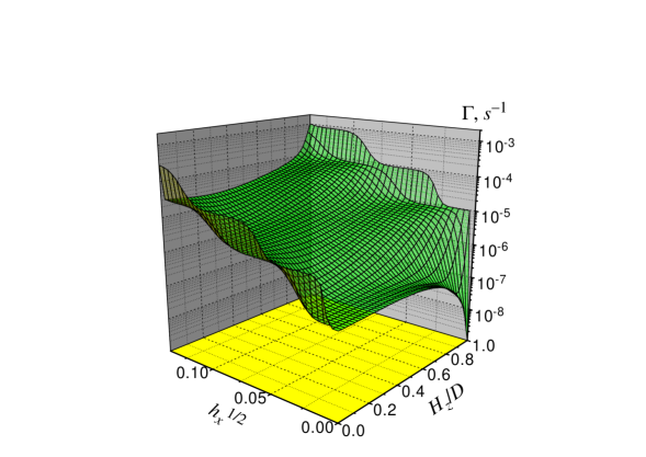
FIG. 6.: Dependence of the escape rate of the uniaxial spin model on the field components $H_{x}$ and $H_{z}$ (parameters are appropriate for Mn₁₂Ac).

\begin{picture}(11.0,7.0)\centerline{\hbox{\psfig{angle=-90,width=341.43306pt}}} \end{picture}

FIG. 7.: Longitudinal field dependence of the escape rate of a large-spin uniaxial model in the fixed transverse field. The curve 1 was obtained from the pure thermoactivation curve $h_{x}=0$ using Eq. (80) for the barrier lowering in the transverse field $h_{x}=0.1$.

Apart from resonant tunneling, the overall shape of $\Gamma(H_{x},H_{z})$ follows approximately the Arrhenius law with the classical barrier height $U(H_{x},H_{z})$. This can be seen especially clear for systems with large spin, frequency-independent relaxation rates and low temperatures. The last condition is needed to reduce the relative role of the field dependence of the prefactor $\Gamma_{0}=\Gamma_{0}(H_{x})$ in the classical expression for $\Gamma$, which is not yet well established (see Refs. [60] and [61]). The comparison of our calculation with the classical result accounting only for the dependence

$$U(H_{x},H_{z})\cong DS^{2}(1-h_{z})^{2}\left[1-2h_{x}\frac{(1-h_{z}^{2})^{1/2}}{(1-h_{z})^{2}}\right]$$ (80)

for $h_{x}\ll 1$ is presented in Fig. 7. The rather good accordance between the classical and quantum results illustrates the conjectures of Sec. II in a more general biased case.

The resonant tunneling curves obtained above do not fully explain the experimental observations [14, 17, 18, 19, 20] showing that all peaks have approximately the same form. The latter can be the consequence of the averaging effect due to the misalignment of the particle’s axes in not perfectly oriented polycrystalline samples. A similar effect can be caused in Mn₁₂Ac by nuclear spins whose fluctuating transverse components can, in addition, induce tunneling even in the absense of an externally applied field $H_{x}$. The corresponding adjustments of our method will be made below.

\begin{picture}(11.0,7.0)\centerline{\hbox{\psfig{angle=-90,width=341.43306pt}}} \end{picture}

FIG. 8.: Resonant tunneling escape rate in Mn₁₂Ac due to nuclear spins and the crystallite misalignments.

In a Mn₁₂Ac molecule each of 12 Mn atoms interacts with its own nuclear spin ${\bf I}_{i}$, $I=5/2$, via the hyperfine (HF) interaction. For the total cluster spin this interaction can be approximately written as

$${\cal H}_{\rm HF}\simeq-A_{\rm eff}{\bf S}{\bf I}_{\rm tot},\qquad{\bf I}_{\rm tot}\equiv\sum_{i}{\bf I}_{i}.$$ (81)

In fact, the hyperfine interactions are somewhat different for different Mn atoms, and their extensive discussion can be found in Ref. [40]. If all the nuclear spins are aligned in the same direction, the energy of the HF interaction $E_{\rm HF,max}\simeq 12ISA_{\rm eff}\simeq 0.6$ K is comparable to the level spacing near the top of the barrier $|\omega_{m+1,m}|\sim 2Dm\sim 1$ K and is much greater than the dipole-dipole energy $E_{d}\simeq 0.06$ K. The effective HF field produced by the nuclei on the cluster spin is in this case about $H_{\rm HF,max}\simeq E_{\rm HF,max}/(g\mu_{B}S)\simeq 0.05$ T. If this HF field is perpendicular to the easy axis $z$, the corresponding dimensionless transverse field $h_{x,{\rm HF}}=g\mu_{B}H_{\rm HF,max}/(2SD)\simeq 3.7\times 10^{-3}$ should result in strong resonant (as well as nonresonant) tunneling; see Fig. 4. On the other hand, the role of the $z$ component of the HF field in resonant tunneling is determined by the dimensionless parameter $g\mu_{B}H_{\rm HF,max}/D\simeq 0.075$. This shows that the narrow resonance lines in Fig. 4 should be averaged away by the fluctuating $z$ component of the hyperfine field; i.e., the hyperfine interaction suppresses the coherence. This second effect was discussed by several authors; [15] here we will take into account both effects of nuclear spins with the help of simplified qualitative arguments.

The subtlety of the hyperfine interaction is that it conserves the total projection $S_{z}+\sum_{i}I_{iz}$, and, strictly speaking, the coupled equations of motion for the tunneling cluster spin and rotating nuclear spins should be solved. In the Arrhenius regime, however, tunneling occurs near the top of the barrier where it is rather fast — it ranges from $\Omega_{mm^{\prime}}\sim|\omega_{m+1,m}|$ off resonance to $\Omega_{mm^{\prime}}\sim\Gamma_{mm^{\prime}}$ at resonance. This is much faster than the nuclear relaxation rate which is due to the fluctuating magnetic fields and is determined by the small nuclear magnetic moment. Further, tunneling of the cluster spin near the top of the barrier leads to a relatively small change of its $z$-projection: $\Delta S_{z}\simeq 2m_{b}\ll 2S$. This is not a large part of the whole integral of motion $S_{z}+\sum_{i}I_{iz}$. Indeed, for the randomly oriented nuclear spins the second term of this sum is on average of order $\sqrt{12}I\simeq 8.7$, and thus tunneling of the cluster spin can be compensated by the corresponding rotation of the nuclear spins. (On the contrary, for tunneling from the ground state at $T\leq T_{0}$ the $z$ projection change is $\Delta S_{z}=2S=20$, and this process cannot go via the interaction with the nuclear spins — it is blocked by the conservation law.) Thus, in the Arrhenius regime one can qualitatively consider nuclear spins as frozen — they do not change their state as a result of the tunneling of the cluster spin. The distribution function of the HF field on the cluster spin can be easily found. As the energy of the interaction of one nuclear spin with the cluster spin $ISA_{\rm eff}\simeq 0.05$ K is much smaller than temperature, one can use the infinite-temperature distribution function for the individual nuclear spins. Then, for a large number of nuclear spins, $N=12\gg 1$, the quantum-statistical averages of the total nuclear spin ${\bf I}_{\rm tot}$ in Eq. (81) are given by the Gaussian distribution function

$$F({\bf I}_{\rm tot})=\frac{1}{(2\pi\sigma_{I})^{3/2}}\exp\left(-\frac{I_{\rm tot}^{2}}{2\sigma_{I}}\right),$$ (82)

where the dispersion $\sigma_{I}=(N/3)I(I+1)$ can be checked calculating the average $\langle I_{{\rm tot},z}^{2}\rangle$ directly and from Eq. (82) and comparing the results. Now, all the previously obtained expressions for the escape rate $\Gamma$, as well as such quantities as the time dependence of magnetization and dynamic susceptibility, should be averaged with the distribution function $F$. In the absense of an externally applied field $H_{x}$, the averaging of each quantity $A(H_{x},H_{z})$ is done explicitly as

$$\bar{A}(H_{x},H_{z})=\!\int\limits_{0}^{\infty}\!\!dx\;2xe^{-x^{2}}\!\!\!\int\limits_{-\infty}^{\infty}\!\!\!dz\;\frac{e^{-z^{2}}}{\pi^{1/2}}A(x\bar{H}_{\rm HF},H_{z}\!+\!z\bar{H}_{\rm HF}),$$ (83)

$$\bar{H}_{\rm HF}=H_{\rm HF,max}\frac{(2\sigma_{I})^{1/2}}{NI},\qquad H_{\rm HF,max}=\frac{NIA_{\rm eff}}{g\mu_{B}}.$$ (84)

The results of this averaging for the escape rate $\Gamma$ are presented in Fig. 8. The role of nuclear spins in inducing resonant tunneling and suppressing the narrow resonance lines is clearly seen. In addition, we have taken into account small fluctuations of the directions of the anisotropy axes of Mn₁₂Ac molecules in polycrystalline samples with the dispersion of only $\Delta\theta=3^{\circ}$. These misalignments also produce a static fluctuating components of the transverse field, and their role becomes progressively more important with the increase of the bias field $H_{z}$. One can see that when all these effects are taken into account, all the resonant tunneling peaks become approximately of the same form, as observed in experiments.

VIII Discussion

We have presented the theory of thermally activated resonant spin tunneling. The bulk of the theory applies to any molecular magnet, while particular numerical illustrations were made for Mn₁₂Ac. Quantization of spin levels, which is the key to explaining experimental results, has dictated our choice of theoretical apparatus. Rather than employing instanton methods, suitable for models with continuous spectra, we have used the density matrix description of the spin interacting with thermal bath.

In continuous models three regimes for the escape rate $\Gamma$ are usually studied. At high temperatures quantum-mechanical effects are not important, and the escape over the barrier is due to pure thermal activation described by the Arrhenius law. In the limit of zero temperature only tunneling out of the ground state is important. There is also an intermediate regime which combines thermal activation to excited levels with tunneling across the barrier, which is called thermally assisted tunneling. In that regime the position of the narrow group of levels which dominate the escape rate depends on temperature, moving continuously from the ground state at $T=0$ to the top of the barrier at the temperature called the crossover temperature. This situation describes a conventional, smooth, second-order transition from quantum tunneling to thermal activation. [57] In principle that transition can also be first order, which would correspond to the sharp crossover from quantum tunneling to thermal Arrhenius-type behavior. [56] We have demonstrated that this is exactly what happens for a spin system in low transverse field. Correspondingly, the experimental study of the escape rate should find the evolution from sharp to smooth crossover between thermally assisted tunneling and the Arrhenius regime on the transverse field.

In systems of moderate spin, such as Mn₁₂Ac, thermally assisted tunneling occurs in a rather narrow temperature range. In experiments the Arrhenius law that occurs in a wider temperature range has been observed. Despite the purely classical temperature dependence of the relaxation in the Arrhenius regime, the field dependence of $\Gamma$ shows quantum effects due to the discrete nature of spin ignored in continuous models. Contrary to these models, which start with a given barrier, a well-defined barrier does not exist for a mesoscopic spin; its effective value depends on the bias field $H_{z}$ in a nonmonotonic manner. The observed minima of the effective barrier are due to the crossing of the spin levels, which results in resonant tunneling between the wells. This is different from a classical spin system where the barrier monotonically decreases with increasing $H_{z}$. This regime can be called thermally activated tunneling, as different from the regime of thermally assisted tunneling. The difference between the two regimes is that in the first regime tunneling always occurs at the top of the barrier, while in the second regime it occurs from excited levels between the bottom and the top of the barrier.

The theory predicts that each resonance in the escape rate $\Gamma$ has a multitower structure with peaks of decreasing width mounting on top of each other. This effect is due to resonant spin tunneling between different matching levels. All peaks are centered at the same field, if the corresponding pair of levels match at the same value of the bias field. Note that this assumpion relies on the simple form of the Hamiltonian used in our calculations. Additional terms of different symmetry would violate this assumtion. If these terms are small, as they are in Mn₁₂Ac, the resonances on $H_{z}$ will not be exactly equidistant and the centers of peaks towering in each resonance must be slightly displaced with respect to each other. The number of peaks in each resonance increases with decreasing dissipation.

Depending on the number $k$ of the resonance [see Eq. (2)], the leading contribution to the rate appears in even or odd orders of the perturbation theory on the transverse field $H_{x}$. This results in the alternation of the shape of resonances on $H_{z}$. Another effect predicted by the theory is the stepwise dependence of the rate on the transverse field when the longitudinal field is tuned to the resonance.

The origin of the terms in the Hamiltonian responsible for tunneling is different for different molecular magnets. The absense of any selection rules for resonances in Mn₁₂Ac unambiguously points to transverse fields causing the transitions. These fields originate from the hyperfine and, to a smaller degree, from the dipole-dipole interactions. In Fe₈ the hyperfine interactions are negligible, and the transitions are presumably caused by the transverse anisotropy.

Our theory for Mn₁₂Ac can pretend to the quantitative description of the magnetic relaxation in this system, as it takes into account all major contributions to the effect. However, observation of more subtle effects, such as the multitower structure of resonances, the alternating shape, stepwise dependence on the transverse field, etc., is less likely in Mn₁₂Ac. This is because of the smearing of these effects by strong fluctuations of the hyperfine field. Fe₈ (see, e.g., Ref. [62]) seems to be a better candidate for observing these effects.

REFERENCES

- [1] A. O. Caldeira and A. J. Leggett, Ann. Phys. (N.Y.) 149, 374 (1983).
- [2] J. Clarke, A. N. Clelend, M. H. Devoret, D. Esteve, and J. M. Martinis, Science 239, 992 (1988).
- [3] See, e.g., J. Tejada and X. X. Zhang, in Quantum Tunneling of Magnetization, edited by L. Gunther and B. Barbara (Kluwer, Dordrecht, 1995).
- [4] D. D. Awshalom, J. F. Smyth, G. Grinstein, D. P. DiVincenzo, and D. Loss, Phys. Rev. Lett. 68, 3092 (1992).
- [5] S. Gider, D. D. Awshalom, T. Douglas, S. Mann, and M. Chaprala, Science 268, 77 (1995).
- [6] W. Wernsdorfer, B. Doudin, D. Mailly, K. Hasselbach, A. Benoit, J. Meier, J.-Ph. Ansermet, and B. Barbara, Phys. Rev. Lett. 77, 1873 (1996).
- [7] W. Wernsdorfer, E. Bonet Orozco, K. Hasselbach, A. Benoit, B. Barbara, N. Demoncy, A. Loiseau, and D. Mailly, Phys. Rev. Lett. 78, 1791 (1997).
- [8] T. Lis, Acta Crystallogr. B 36, 2042 (1980).
- [9] R. Sessoli, D. Gatteschi, A. Caneschi, and M. A. Novak, Nature 365, 141 (1993).
- [10] M. A. Novak and R. Sessoli, in Quantum Tunneling of Magnetization, edited by L. Gunther and B. Barbara (Kluwer, Dordrecht, 1995).
- [11] A. Caneschi, D. Gatteschi, R. Sessoli, A. L. Barra, L. C. Brunel, and M. Guillot, J. Am. Chem. Soc. 117, 301 (1991).
- [12] R. Sessoli, Mol. Cryst. Liq. Crist. 274, [801]/145 (1995).
- [13] M. Hennion, L. Pardi, I. Mirebeau, E. Suard, R. Sessoli, and A. Caneschi, Phys. Rev. B (to be published 1 September 1997).
- [14] J. R. Friedman, M. P. Sarachik, J. Tejada, and R. Ziolo, Phys. Rev. Lett. 76, 3830 (1996).
- [15] A. Garg, Phys. Rev. Lett. 74, 1458 (1995).
- [16] C. Paulsen and J.-G. Park, in Quantum Tunneling of Magnetization, edited by L. Gunther and B. Barbara (Kluwer, Dordrecht, 1995).
- [17] J. M. Hernández, X. X. Zhang, F. Luis, J. Bartolomé, J. Tejada, and R. Ziolo, Europhys. Lett. 35, 301 (1996).
- [18] L. Thomas, F. Lionti, R. Ballou, D. Gatteschi, R. Sessoli, and B. Barbara, Nature 383, 145 (1996).
- [19] J. M. Hernández, X. X. Zhang, F. Luis, J. Tejada, J. R. Friedman, M. P. Sarachik, and R. Ziolo, Phys. Rev. B 55, 5858 (1997).
- [20] F. Lionti, L. Thomas, R. Ballou, B. Barbara, A. Sulpice, R. Sessoli, and D. Gatteschi, J. Appl. Phys. 81, 4608 (1997).
- [21] S. M. J. Aubin, D. N. Hendrickson, S. Spagna, R. E. Sager, H. J. Eppley, and G. Christou, (unpublished).
- [22] J. R. Friedman, M. P. Sarachik, J. M. Hernández, X. X. Zhang, J. Tejada, E. Molins, and R. Ziolo, J. Appl. Phys. 81, 3978 (1997).
- [23] F. Luis, J. Bartolomé, J. F. Fernández, J. Tejada, J. M. Hernández, X. X. Zhang, and R. Ziolo, Phys. Rev. B 55, 11448 (1997).
- [24] E. M. Chudnovsky and J. R. Friedman (unpublished).
- [25] D. A. Garanin, J. Phys. A 24, L61 (1991).
- [26] A. L. Barra, D. Gatteschi, and R. Sessoli, Phys. Rev. B (to be published 1 October 1997).
- [27] E. M. Chudnovsky and L. Gunther, Phys. Rev. Lett. 60, 661 (1988).
- [28] M. Enz and R. Schilling, J. Phys. C 19, L711 (1986).
- [29] O. B. Zaslavskii, Phys. Lett. A 145, 471 (1990).
- [30] J. L. van Hemmen and A. Sütő, Europhys. Lett. 1, 481 (1986).
- [31] J. L. van Hemmen and A. Sütő, Physica B 141, 37 (1986).
- [32] G. Scharf, W. F. Wreszinski, and J. L. van Hemmen, J. Phys. A 20, 4309 (1987).
- [33] I. Ya. Korenblit and E. F. Shender, Zh. Eksp. Teor. Fiz. 75, 1862 (1978) [JETP 48, 937 (1978)].
- [34] F. Hartmann-Boutron, J. Phys. I 5, 1281 (1995).
- [35] L. Schatzer, W. Breymann, and H. Thomas, Z. Phys. B 101, 131 (1996).
- [36] J. R. Friedman, Ph. D. thesis, City University of New York, 1996.
- [37] J. Villain, F. Hartmann-Boutron, R. Sessoli, and A. Rettori, Europhys. Lett. 27, 159 (1994).
- [38] A. Abragam and A. Bleaney, Electron Paramagnetic Resonance of Transition Ions (Clarendon Press, Oxford, 1970).
- [39] N. G. Koloskova, in Spin Lattice Relaxation in Ionic Solids, edited by A. A. Manenkov and R. Orbach (Harper and Row, New York, 1966), p. 232.
- [40] F. Hartmann-Boutron, P. Politi, and J. Villain, Int. J. Mod. Phys. B 10, 2577 (1996).
- [41] P. Politi, A. Rettori, F. Hartmann-Boutron, and J. Villain, Phys. Rev. Lett. 75, 537 (1995).
- [42] D. A. Garanin, Phys. Rev. E 55, 2569 (1997).
- [43] S. Nakajima, Prog. Theor. Phys. 20, 948 (1958).
- [44] R. Zwanzig, J. Chem Phys. 33, 1338 (1960).
- [45] R. Zwanzig, Phys. Rev. 124, 983 (1961).
- [46] H. Grabert, Projection Operator Techniques in Nonequilibrium Statistical Mechanics (Springer, Berlin, 1982).
- [47] V. Romero-Rochin, A. Orsky, and I. Oppenheim, Physica A 156, 244 (1989).
- [48] D. A. Garanin, Physica A 172, 470 (1991).
- [49] R. Orbach, Proc. Roy. Soc. London, Ser. A 264, 458 (1961).
- [50] A. J. Leggett, S. Chakravarty, A. T. Dorsey, M. P. A. Fisher, A. Garg, and W. Zwerger, Rev. Mod. Phys. 59, 1 (1987).
- [51] A. Garg, Phys. Rev. B 51, 15161 (1995).
- [52] H. A. Kramers, Physica 7, 284 (1940).
- [53] W. F. Brown, Jr., Phys. Rev. 130, 1677 (1963).
- [54] D. A. Garanin, V. V. Ishchenko, and L. V. Panina, Teor. Mat. Fiz. 82, 242 (1990) [Theor. Math. Phys. 82, 169 (1990)].
- [55] D. A. Garanin, Phys. Rev. E 54, 3250 (1996).
- [56] E. M. Chudnovsky, Phys. Rev. A 46, 8011 (1992).
- [57] I. Affleck, Phys. Rev. Lett. 46, 388 (1980).
- [58] A. I. Larkin and Yu. N. Ovchinnikov, Pis’ma Zh. Eksp. Teor. Fiz. 37, 322 (1983) [JETP Lett., 37 382 (1983)].
- [59] R. Rose, S. Han, and J. E. Lukens, Phys. Rev. Lett. 75, 1614 (1995).
- [60] W. F. Brown, Jr., IEEE Trans. Magn. MAG-15, 1196 (1979).
- [61] W. T. Coffey, D. S. F. Crothers, J. L. Dormann, L. J. Geoghegan, Yu. P. Kalmykov, J. T. Waldron, and A. W. Wickstead, Phys. Rev. B 52, 15951 (1995).
- [62] C. Sangregorio, T. Ohm, C. Paulsen, R. Sessoli, and D. Gatteschi, Phys. Rev. Lett. 78, 4645 (1997).