Phase-Disorder Effects in a Cellular Automaton Model of Epidemic Propagation

Abstract

A deterministic cellular automaton rule defined on the Moore neighbourhood is studied as a model of epidemic propagation. The directed nature of the interaction between cells allows one to introduce the dependence on a disorder parameter that determines the fraction of “in-phase” cells. Phase-disorder is shown to produce peculiar changes in the dynamical and statistical properties of the different evolution regimes obtained by varying the infection and the immunization periods. In particular, the finite-velocity spreading of perturbations, characterizing chaotic evolution, can be prevented by localization effects induced by phase-disorder, that may also yield spatial isotropy of the infection propagation as a statistical effect. Analogously, the structure of phase-synchronous ordered patterns is rapidly lost as soon as phase-disorder is increased, yielding a defect-mediated turbulent regime .

PACS numbers: 87.10.+e; 63.10.+a

I Introduction

Deterministic Cellular Automata (DCA) have revealed very useful tools for characterizing some basic complex behaviours emerging from simple, local evolution rules. On the other hand, they are not particularly suitable for applications, mainly because they are independent of some tunable parameter. This is why the mechanisms of front propagation in epidemics, forest fires and chemical oscillations are usually modelled on the basis of probabilistic CA rules (see, for instance [1, 2]). Probability plays the role of a control parameter, that may yield interesting phenomena like phase transitions between different dynamical regimes (e.g., spiral-wave versus fully developed turbulence or extinction versus ordered front propagation).

A similar and equally interesting scenario has been recently obtained for a 3-state DCA rule of directed epidemic propagation in 2d [3] . In this model the state-space of each cell is extended to a phase variable that allows for introducing a “quenched-disorder” parameter.

The complete definition of the model introduced in [3] and a summary of the main results therein obtained is contained in Section 2. The extension of the model to nearest- and next-to-nearest neighbour interaction is discussed in Section 3, where the different dynamical regimes, characterizing the “phase-synchronous” case, are also enlisted. The main difference with respect to the model considered in[3], where the interaction was limited to nearest-neighbour cells, is that the mechanism of infection propagation in the chaotic regime is characterized by two typical speeds, associated to the anysotropy of the interaction induced by the lattice. Section 4 is devoted to a detailed account of the effects induced by quenched phase-disorder on both chaotic and ordered dynamical regimes. In particular, we show that there are chaotic regimes where sufficiently small values of the phase-disorder paramter can inhibit the spreading of perturbations at finite velocity. If this localization effect is absent, one obtains that, at some finite value of the phase-disorder parameter, the isotropy of the infection mechanism can be restored as a statistical effect. Moreover, we find that the structure of phase-synchronous ordered patterns is rapidly lost as soon as $p$ is decreased. Such a phenomenon is strongly reminiscent of the transition from a weakly-turbulent regime to a strongly-turbulent one, already abserved in lattices of coupled stable maps [4].

Conclusions are drawn in Section 5.

II The Model

The DCA model is defined on a square lattice of size $L\times L$ with periodic boundary conditions. Each cell can assume three different states : infected ($I$), susceptible ($S$) and immunized, or quiescent ($Q$). Its neighbourhood is made of ${\cal N}$ cells. The model depends on two main parameters: $T_{I}$ and $T_{Q}$, the infection and immunization periods, respectively. As we have already pointed out in the introduction, each cell depends also on a phase variable $\theta=1,\cdots,{\cal N}$. At each instant of time $t$, any cell interacts with only one of the cells in its neighbourhood, that is selected by the value of $\theta(t)$.

The deterministic updating rule is defined as follows :

• If the phase variable of an $I$-cell selects a $S$-cell, this becomes an $I$-cell at the following time step.

• The infection (immunization) time of an $I$- ($Q$) -cell is increased by a unit time step, so that after a period of $T_{I}$ ($T_{Q}$) steps an $I$- ($Q$)-cell becomes a $Q$- ($S$)-cell.

• Independently of the state of the cell, its phase variable is increased by one unit. Accordingly, as time flows $\theta$ spans sequentially all the cells in the neighbourhood, turning back to its initial value after ${\cal N}$ time steps.

The presence of the phase variable $\theta$ allows one to introduce the quenched-disorder parameter $p$, measuring the fraction of cells sharing the same initial phase value $\theta(0)$. According to R3, these cells will then share the same phase value at each instant of time. In the “phase-synchronous” case, $p\,=\,1$, all cells have the same phase value. For $1/{\cal N}\leq p\leq 1$, a fraction of $p$ randomly chosen cells have the same phase value, while the remaining cells equally and randomly share the other ${\cal N}-1$ phase values.

This 2-d epidemic propagation model was studied for ${\cal N}=4$ (Von Neumann neighbourhood) by Giorgini et al. [3]. Let us summarize the main results, introducing the same symbolic notations used in the quoted reference.

First of all the authors classified the different dynamical regimes characterizing the phase-synchronous case ($p=1$), when both $T_{I}$ and $T_{Q}$ are varied. To this aim, they considered a specific initial condition with a single $I$-cell in a “sea” of $S$-cells. For small values of $T_{I}$ (smaller than or equal to ${\cal N}/2$) and for $T_{Q}$ large enough (at least larger or equal to ${\cal N}/2$), the epidemy, after a transient period of time, dies out (extinction regime, symbolically denoted by E). Actually, a cluster of $I$-cells develops quite soon, but its further propagation is inhibited by the $Q$-cells that, after a sufficient time span, form at its boundary. For smaller values of $T_{Q}$, the infection remains confined inside a finite lattice region centered around the initially infected cell: the cluster of $I$-cells is characterized by a localized periodic evolution (symbol P). Note that now the extinction of the infection does not occur, because the periodicity of the phase variable allows for the re-infection of previously infected cells, that had already turned to $Q$-cells, according to R2. For large values of $T_{I}$ and $T_{Q}$, the propagation of ordered fronts sets in (symbol F). The re-infection effect is absent and $I$-cells propagate indefinitely as an ordered front, preserving the lattice square symmetry. It is straightforward to realize that in a finite size lattice such a front propagation dies out after reaching the boundaries.

The interference of propagating fronts yields a seemingly chaotic evolution (symbol D), in which both the basic mechanism (front propagation and re-contamination) are present and produce space time patterns that do not exhibit any regularity. Note that such an outcome cannot be considered as totally unexpected, since it has been shown that, according to very general hypotheses, DCA rules with a state space larger than boolean may give rise to such non-trivial behaviours [5].

The quantity used in [3] for obtaining a first characterization of the statistical properties associated to the D-regime was

$$b(t)\,=\,{{\delta(t)}\over{I(t)\,S(t)}}$$ (1)

where $\delta(t)$ is the number (normalized to the lattice size $L^{2}$) of $I$-cells interacting at time $t$ with $S$-cells according to R1, while $I(t)$ and $S(t)$ represent the ratios of infected and susceptible cells at the same time, respectively. In practice, $b(t)$ can be interpreted as a measure of the rate of propagation of information through the lattice, or, equivalently, of the inhomogeinity of the cell-state distribution. It was found to exhibit robust statistical properties in the D regime (self-averaging): the hystogram of the frequency of occurrence of $b$ values vs. $b$ (i.e., the normalized probability distribution $P(b)$ ) is a gaussian-like function.

It is worth stressing that any DCA rule must eventually yield a periodic evolution on a finite-size lattice. Nonetheless, one can conjecture that the “transient” chaotic evolution typical of the D-regime would last forever in the thermodynamic limit ($L\rightarrow\infty$). Following [6], this could be directly verified by measuring how the average duration of the D-regime increases with $L$. Since such a strategy is practically impossible to be worked out satisfactorily for large enough 2-d samples, the effective unpredictability of the D-regime can be detected indirectly by measuring a finite average damage spreading velocity $\langle v_{d}\rangle$. A reliable determination of its value can be obtained by the following procedure. One can start from a randomly seeded initial condition, obtained by assigning to all cells some normalized probabilities of being in the states $S$, $I$ and $Q$. After a sufficiently long transient time, any initial condition evolves to an irregular space-time pattern whose statistical features (e.g., $P(b)$) are found to be independent of the initial condition. A spatially localized perturbation of finite amplitude is introduced in one of these patterns and the evolution of the difference field with respect to the unpertubed pattern is then determined by measuring at each instant of time $t$ the radius $R(t)$ of the smallest circle where the difference field is non-zero. The averaging over a suitable set of initial conditions yield a reliable determination of

$$\langle v_{d}\rangle={{d\langle R(t)\rangle}\over{dt}}$$ (2)

For $p=1$ one observes $\langle v_{d}\rangle\not=0$ in the D-regime; decreasing $p$, $\langle v_{d}\rangle$ is found to approach zero at some finite value $p_{c}$, indicating the occurrence of a continuous transition to a dynamical phase, where, as an effect of the phase-disorder, perturbations remains localized.

III The Moore-neighbourhood case

We have extended the model described above to next-to-nearest neighbour interaction (${\cal N}=8$).

Let us point out the main differences of this model with respect to the case studied in [3]:

• - two velocities of propagation of the infection mechanism along the main axes (nearest neighbour interaction) and along the diagonals (next-to-nearest neighbour interaction) of the square lattice are present;

• - the commensurability relations of ${\cal N}$ with $T_{I}$ and $T_{Q}$ have changed.

As we shall see, such features introduce some peculiar changes. On the other hand, the basic mechanisms of re-contamination (infection of a previously infected cell) and front propagation are found to play the crucial role also in this case.

This is confirmed by the study of the dynamical regimes characterizing this DCA rule for $p=1$, when $T_{I}$ and $T_{Q}$ are varied. Numerical simulations have been performed for $L=400$, starting from the initial condition of one $I$-cell in a “sea” of $S$-cells . The various dynamical regimes and the phase diagram are reminiscent of those observed in the 4-neighbours case, although, as expected, they occur at different values of the parameters. They are summarized in Table 1 .

	$T_{I}$
$T_{Q}$	2	3	4	5	6	7	8	9	10	11
1	P	P	P	D	P	P	D	P	P	P
2	P	P	P	D	P	D	D	P	P	F
3	P	P	P	P	D	D	D	D	F	F
4	P	P	P	E	D	D	D	F	F	F
5	P	P	E	E	D	D	F	F	F	F
6	P	E	E	E	D	F	F	F	F	F
7	E	E	E	E	P	F	F	F	F	F
8	E	E	E	E	P	F	F	F	F	F
9	E	E	E	E	P	F	F	F	F	F
10	E	E	E	E	F	F	F	F	F	F

Table 1 - D: disordered evolution, E: extinction, F: ordered front propagation, P: periodic evolution.

As shown for the ${\cal N}=4$ case, we have characterized the D-regime by computing the damage-spreading velocity (2), that is found to be a positive constant for $t$ large enough (e.g, see Figure 1).

FIG. 1.: $\langle R\rangle$ as a function of $t$ for $p=1$ and $T_{I}=8$, $T_{Q}=1$ (dotted line), $T_{I}=7$ ,$T_{Q}=5$ (full line); averages are made over 100 initial conditions.

When starting from a randomly seeded initial condition, also in the dynamical regimes different from D the initial randomness may be apparently maintained during the evolution (apart some cases observed in the P regime, where the space-time pattern can be seen to rapidly “freeze” into a periodic evolution). On the other hand, in all of these cases one finds $\langle v_{d}\rangle=0$. This shows that this quantity is a reliable order parameter and confirms that the propagation of information is the main non-linear mechanism yielding unpredictable evolution in DCA.

In the following section we are going to describe in some detail the effects of variyng $p$ in the different regimes, while taking into account in this perspective measurements of both $\langle v_{d}\rangle$ and $b(t)$.

IV The Effects of Quenched Phase-Disorder

A Chaotic Evolution for small $T_{Q}$

For small values of the immunization period $T_{Q}$ one expects that phase-disorder may not affect the main features of a D-regime. In fact, this guess is confirmed by numerical simulations. Here we consider just the case $T_{I}=8$ and $T_{Q}=1$ as a typical example. For what concerns the initial state of the cells we have considered both kinds of initial condition described in the previous section, verifying that they yield the same asymptotic evolution. In particular, the time-averaged values of the density of $I$-cells and of $Q$-cells are found to approach asymptotic values independent of the chosen initial condition.

We have measured the damage spreading velocity $\langle v_{d}\rangle$ for different values of $p$.

FIG. 2.: The average damage spreading velocity $\langle v_{d}\rangle$ of the difference pattern for $T_{I}=8$, $T_{Q}=1$ (dotted lines), $T_{I}=7$ ,$T_{Q}=5$ (full lines); the different lines correspond to ensemble averages performed over 100 initial conditions and time averages performed over the last 500 points for t=500, 1000 and 2000 (from top to bottom).

Fig.2 shows that $\langle v_{d}\rangle$ has a finite value, that does not vary significantly in the whole range of $p$. This indicates that phase-disorder, in this case, is unable to compete with the mechanism of infection propagation. Conversely, it is found to progressively remove the anisotropy of the interaction when $p$ is decreased, thus increasing the efficiency of the epidemic propagation. This conclusion can be drawn by measuring $b(t)$. Specifically, the hystogram of the frequency of occurrence of $b$ values vs. $b$ (i.e., the normalized probability distribution $P(b)$ ) averaged over an hundred of initial conditions is shown in Fig.3.

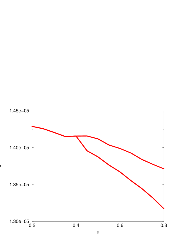
FIG. 3.: At the top: the probability distribution $P(b)$ for $T_{I}=8$ and $T_{Q}=1$ and for three different values of $p$; it has been obtained averaging over 100 initial conditions. At the bottom: the position of the maxima is reported as a function of $p$, showing that collapse occurs at $p\approx 0.4$ .

For high values of $p$, including the case $p=1$, $P(b)$ exhibits two separated peaks. We have verified that they are in correspondence with infection propagation along the lattice axis ( the right one ) and along the diagonal (the left one ). Decreasing $p$ the two peaks of the distribution approach one another, until they merge in a unique distribution at $p\approx 0.4$.

This is definitely the main outcome of our analysis of the D-regime for small values of $T_{Q}$: the restoration of the isostropy of the epidemic propagation due to phase-disorder occurs at a finite value of $p$ through an inverse-bifurcation mechanism concerning the probability distribution $P(b)$. This is highly non trivial, since the bifurcation applies to a ”statistical” observable and not just to a single dynamical variable. Upon these results, one is led to conclude that small immunization times prevent the possibility of estinghuishing the epidemy, while disorder can make the mechanism even more efficient by restoration of isotropy. Actually, when $p$ is lowered the unique peak of the distribution displaces towards larger values of $b$.

B Chaotic Evolution for large $T_{Q}$

A different scenario, similar to the one associated to the phase transition described in [3] when $p$ varies, is expected to be observed in the D-regime for larger values of $T_{Q}$. As an example, we discuss here the case $T_{I}=7$ and $T_{Q}=5$. The numerical measurements of $\langle v_{d}\rangle$ versus $p$ (see Fig. 2) allow us to locate a critical values at $p_{c}\approx 0.5$ . Below $p_{c}$ the damage spreading velocity $\langle v_{d}\rangle$ vanishes, thus indicating that, at variance with the previous case, now there is a dynamical phase, where disorder is able to localize the infection in some lattice region. A similar feature is not peculiar of DCA, but it was found also, for instance, in coupled map lattices, where quenched disorder is able to inhibit chaotic diffusion [7].

The shape of the curve reported in Fig. 2 gives evidence of a continuous transition. Note that a numerical determination of the critical exponents is practically unfeasible, due to finite size effects that would demand exceedingly large values of $L$.

On the other hand, in this case the hystogram of $P(b)$ exhibits a two-peak structure that is maintained up to $p_{min}=0.125$. Nonetheless, when $p$ is decreased the two peaks tend to approach each other, still shifting towards higher average values of $b(t)$. Accordingly, the anisotropy of the epidemic propagation is intrinsic to this dynamical regime, although the propagation of finite amplitude perturbations for $p<p_{c}$ is prevented by localization effects induced by the phase-disorder.

C Ordered Evolution for $T_{I}\approx T_{Q}$

Phase-disorder is expected to modify also the dynamical features of the ordered regimes. For the sake of space, let us consider here just the interesting case $T_{I}=7$ and $T_{Q}=6$, where the evolution is front-like (F) for $p=1$. The remarkable result is that disorder, now, yields a qualitative change in the dynamics passing from a front-propagation scenario to a spatially disordered evolution as soon as $p$ is decreased below 1. The average damage spreading velocity $\langle v_{d}\rangle$ remains null for any value of $p$. Nonetheless, phase-disorder is able to prevent the extinction of the epidemy, that , due to boundary effects, occurs for $p=1$ . In Fig. 4 we show a snapshot of a typical spatial pattern of this dynamics for $p=0.2$ .

     

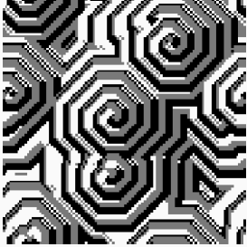
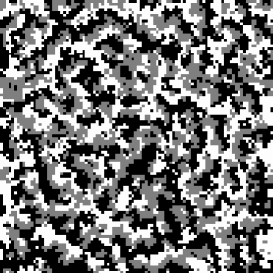
FIG. 4.: Snapshot of the pattern for $T_{I}=7$ and $T_{Q}=6$, $p=1.0$ (left) and $p=0.2$ (right) with random initial conditions

FIG. 5.: Probability distributions $P(b)$ for $p=1$ and $p=0.2$. It exhibits a peculiar peaked structure for $p=0.2$.

When random initial conditions are imposed the system evolves towards ordered structures for $p=1$ (Fig. 4, left) and the propagation mechanism is described by a broad probability distribution $P(b)$ (Fig. 5, full line). For $p=0.2$ random initial conditions yield disordered evolution quite similar to one-infected-site initial conditions (Fig. 4, right) while $P(b)$ mantains multi-peaked structure (Fig.5, dotted line). This can be interpreted as an indication of different propagation mechanisms characterized by different space-time periodicities.

V Conclusions and perspectives

In this paper we have analyzed the effect of disorder over some typical dynamical regimes occurring in an epidemic propagation 8-neighbour DCA model.

In analogy to what already observed in [3], different dynamical regimes including periodic evolution, front propagation and chaotic patterns are observed when the infection and the immunization periods are varied. Here we have performed a more refined analysis of these regimes, while pointing out new features of suh a class of DCA.

In particular, in Sec. 4 we have described three chaotic regimes characterized by different dynamical and statistical properties. Two of them are found to correspond to a D-regime in the phase-synchronous case. In such cases the presence of quenched phase-disorder may yield very different consequences: either a localization transition for the damage spreading velocity or an inverse bifurcation in the probability distribution of the infection rate.

Conversely, the third case occurs just as an effect of increasing phase-disorder applied to the front-propagation regime. A sort of weakly turbulent phase mediated by defects in the form of spiral waves is observed for sufficiently small values of $p$. It is worth stressing that this regime is charecterized neither by propagation of damage nor by a bifurcation-transition in the shape of of $P(b)$. In this sense it could not be interpreted as a truly chaotic case, indicating that it occurs as a complex regime located at the border (in the $(T_{I},T_{Q})$-parameter space) between chaotic and regular evolution. This scenario is definitely reminiscent of what has been observed in coupled stable-map models [4, 8].

REFERENCES

- [1] B. Schönfisch, Physica D 80, 433 (1995).
- [2] N. Boccara, K. Cheong, J. of Phys. A 25, 2447 (1992).
- [3] G. Rousseau, B. Giorgini, R. Livi and H. Chaté, Physica D 103, 554 (1997).
- [4] Y. Cuche, R. Livi ans A. Politi, Physica D 103, 369 (1997).
- [5] C.H. Bennet, G. Grinstein, Y. He, C. Jayaprakash and D. Mukamel, Phys. Rev. A 41, 1932 (1990).
- [6] A. Politi, R. Kapral, R. Livi and G.-L. Oppo, Europhys. Lett. 22, 571 (1993).
- [7] G. Radons, Physical Review Lett. 77, 4748 (1996).
- [8] F. Cecconi, R. Livi and A. Politi, Phys.Rev. E 57, 2703 (1998).