Inhibition of spontaneous emission in Fermi gases

Abstract

Fermi inhibition is a quantum statistical analogue for the inhibition of spontaneous emission by an excited atom in a cavity. This is achieved when the relevant motional states are already occupied by a cloud of cold atoms in the internal ground state. We exhibit non-trivial effects at finite temperature and in anisotropic traps, and briefly consider a possible experimental realization.

5 May 1998

The inhibition and enhancement of spontaneous emission of an atom by embedding it in a cavity has been one of the most striking predictions in the field of cavity QED [1, 2]. Several experiments have and are currently being carried out to test this prediction. The explanation of this phenomenon is very simple: according to Fermi’s golden rule, the spontaneous emission rate $\Gamma$ is proportional to the density of modes of the electro-magnetic field available at the atomic transition frequency; the cavity modifies the mode structure, and therefore this rate. In particular, if all the normal modes of the cavity are far off resonance with respect to the atomic transition frequency, there are no modes available where a photon can be emitted, and therefore spontaneous emission is inhibited.

In this paper we analyze how the spontaneous emission rate $\Gamma$ of an atom can be inhibited by using quantum statistical principles. The idea is to surround a fermionic atom in an internal excited state $|e\rangle$ by a gas formed by identical particles in an internal ground state $|g\rangle$. According to Fermi’s golden rule, $\Gamma$ depends on the occupation number of the different motional states to which the atom can be transferred after spontaneous emission. In particular, if they are already occupied then the atom cannot decay. This can be viewed as well as a simple consequence of Pauli’s exclusion principle. Thus, in analogy to cavity QED one can say that spontaneous emission can be inhibited by reducing the motional “modes” available to the excited atom.

From a qualitative point of view, the inhibition of spontaneous emission can be easily understood. Consider a set of $N$ fermions in the state $|g\rangle$ and one fermion in an excited state $|e\rangle$ that can only decay into $|g\rangle$. Assume, for simplicity, that all the atoms are trapped in a harmonic potential at a given temperature. In this problem there are three energies scales which determine the properties of $\Gamma$. First, $k_{B}T$, the thermal energy of the particles. Second, the Fermi energy $E_{F}$ of the ground state atoms, which is the maximum energy of the fermions at zero temperature. Finally, the recoil energy $E_{R}=\hbar^{2}k_{0}^{2}/2m$ (where $k_{0}$ is the wavevector corresponding to the transition $|e\rangle\rightarrow|g\rangle$ and $m$ is the atom mass), which is the averaged motional energy acquired by the excited atom in the emission process. Typically, the motional states with energies $E\leq E_{F}-k_{B}T$ are occupied, whereas those with $E\geq E_{F}+k_{B}T$ are basically available. Thus, if the initial motional energy of the excited atom plus the one gained in the emission process $\sim k_{B}T+E_{R}\leq E_{F}-k_{B}T$, spontaneous emission will be inhibited. As the temperature decreases or the Fermi energy increases (equivalently, the number of ground state atoms increases) this phenomenon becomes more pronounced. A quantitative analysis of this phenomenon, on the other hand, is much more complicated since in order to evaluate the results given by Fermi’s golden rule one needs to perform heavy numerical calculations. In this paper we have performed these numerical calculations, as well as obtained simple analytical formulas for some interesting regimes. In particular, we have studied the inhibition of spontaneous emission of photons along different spatial directions both for isotropic and cylindrically symmetric traps as a function of the temperature, Fermi energy and anisotropy parameter. We have also analyzed a situation which we think it is closer to the foreseeable experimental possibilities.

We consider an excited atom confined in a harmonic potential at some given temperature $T$. Let us denote by $\Gamma_{0}(\Omega)d\Omega$ the spontaneous emission rate of photons in the solid angle $d\Omega$ around the direction defined by $\Omega$ for a single atom, and by $\Gamma(\Omega)d\Omega$ the corresponding value in the presence of $N$ ground state fermions confined in the same potential at the same temperature $T$. We are interested in the “modification factor” $M_{f}(\Omega)\equiv\Gamma(\Omega)/\Gamma_{0}(\Omega)$ which gives us information about the modification of spontaneous emission along a given direction $\Omega$. Using Fermi’s golden rule we obtain

$$M_{f}(\Omega)=\sum_{\vec{m},\vec{n}=0}^{\infty}P_{\vec{m}}(1-F_{\vec{n}})|\langle\vec{n}|e^{-i\vec{k}(\Omega)\cdot\hat{\vec{r}}}|\vec{m}\rangle|^{2}$$ (1)

Here, $F_{\vec{n}}=(e^{(\hbar\omega/k_{B}T)(\vec{\nu}\cdot\vec{n}-\mu)}+1)^{-1}$ are the Fermi-Dirac and $P_{\vec{m}}=P_{0}e^{-(\hbar\omega/k_{B}T)\vec{\nu}\cdot\vec{m}}$ the Boltzmann distribution for the ground and excited state atoms; $|\vec{n}\rangle=|n_{x}\rangle|n_{y}\rangle|n_{z}\rangle$ denote the eigenstates of the harmonic oscillator with frequencies $(\omega_{x},\omega_{y},\omega_{z})\equiv\omega\vec{\nu}$ along the principal axis [3]. The chemical potential $\mu$ and the number of atoms $N$ can be expressed in terms of $E_{F}$ and $\omega$ in the usual way. Finally, $\vec{k}(\Omega)/k_{0}$ is a unit vector along the direction given by $\Omega$. The interpretation of this formula is very simple. The probability density that the excited atom is transferred from $|\vec{m}\rangle$ to $|\vec{n}\rangle$ by emitting a photon along the direction $\Omega$ is $|\langle\vec{n}|e^{-i\vec{k}(\Omega)\cdot\hat{\vec{r}}}|\vec{m}\rangle|^{2}$. This matrix elements has to be multiplied by the probability that the initial state and the final state are occupied $[P_{\vec{m}}$ and $(1-F_{\vec{n}})]$ and summed over. Note that, in order to determine $M_{f}$, one has to perform six infinite summations for each value of $\Omega$, which in general cannot be evaluated even using a supercomputer. In the following we will consider that $\omega_{z}/\lambda=\omega_{x}=\omega_{y}$, in which case $M_{f}(\Omega)=M_{f}(\theta)$ only depends on the polar angle $\theta$ and the problem becomes tractable numerically. Furthermore, we will also derive some analytical approximations to this formula.

To begin we consider an isotropic trap ($\lambda=1$). In this case, using the spherical symmetry one can show that the emission rate becomes independent of the photon direction and Eq. (1) reduces to

$$M_{f}=\frac{\Gamma}{\Gamma_{0}} = \sum_{n,m=0}^{\infty}P_{m}(1-F_{n})\times$$ (3)

$$\sum_{l=0}^{\min[n,m]}(l+1)|\langle n-l|e^{ik_{0}\hat{x}}|m-l\rangle|^{2}\;,$$

where $\Gamma_{0}$ and $\Gamma$ are the spontaneous emission rates in free space and in the presence of quantum statistical effects, respectively. Now, the states $|n\rangle$ denote one dimensional eigenstates of the harmonic oscillator and $P_{m}$ and $F_{n}$ are the Boltzmann and Fermi distributions at a given energy $n\hbar\omega$. These sums can be performed numerically; the results are shown in Fig. 1 as a function of temperature and Fermi energy. One can see clearly that, as predicted by the simple arguments given above, Fermi inhibition is strongest at low temperatures and large Fermi energies, but does persist at relatively higher temperatures.

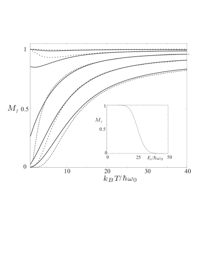
FIG. 1.: $M_{f}$ as a function of temperature, for a trap with $E_{R}=25\hbar\omega$. The solid curves represent Fermi energies ranging in steps of ten from $E_{F}=10\hbar\omega$ (top) to $E_{F}=50\hbar\omega$ (bottom); the dotted curves are the semi-classical approximation. The inset shows $M_{f}$ at $T=0$ as a function of Fermi energy.

At zero temperature the Fermi-Dirac distribution becomes a step function, and the sums in Eq. (3) may be evaluated explicitly. The result is an incomplete Gamma function $M_{f}=\Gamma[E_{F}/(\hbar\omega),E_{R}/(\hbar\omega)]$, whose integral representation expresses the basic competition between Fermi energy and recoil energy [4] We have plotted this result in the inset of Fig. 1. As long as the Fermi energy is much smaller than the recoil energy, the spontaneous emission rate of the atom is not substantially different from the free case; this is because the matrix element in Eq. (3) is concentrated around $n-m=\pm(E_{R}/\hbar\omega)$ (partial conservation of momentum due to the finite strength of the confining potential). So Fermi inhibition at zero temperature is negligible as long as levels around $E_{R}/(\hbar\omega)$ are still unoccupied. Once the Fermi sphere expands beyond these levels, however, the probability of emission drops sharply, since to emit an optical photon and move into an available motional state then requires an improbably large impulse from the trapping potential.

At high temperatures, the sharp edge of the Fermi-Dirac distribution erodes; eventually this means that we can analyze Eq. (3) semi–classically. The matrix element for the $m\to n$ transition is concentrated around the values satisfying $\hbar\omega(n-m)=\pm E_{R}$ with width $\delta E\sim 2(\hbar\omega E_{R})^{1/2}\sqrt{2m}$, where $m\hbar\omega$ is typically $\leq 2k_{B}T$ (otherwise $P_{m}\simeq 0$). On the other hand, the Fermi-Dirac distribution changes appreciably only at energy scales $k_{B}T$, i.e, $F_{n}\simeq F_{n^{\prime}}$ for $\hbar\omega|n-n^{\prime}|\ll k_{B}T$. Thus, if $\delta E\ll k_{B}T$, i.e. $E_{R}\ll k_{B}T$ we can replace $F_{n}\to F_{m\pm E_{R}/(\hbar\omega)}$ in Eq. (1). The sum over $n$ then equals one; and at high temperature we can also approximate the sums over $m$ by integrals, obtaining

$$M_{f}=\frac{\Gamma}{\Gamma_{0}}\doteq e^{\beta(\eta^{2}-E_{F})}\log(1+e^{-\beta(\eta^{2}-E_{F})})$$ (4)

As can be seen from Fig. 1, this approximation is actually quite good even for moderately high temperatures. As $T\to\infty$ the semi-classical result becomes exact, and shows that Fermi inhibition disappears in the classical limit, when the chance of any particular level being occupied becomes infinitesimal. By combining this observation with the fact that for $E_{F}<E_{R}$ Fermi inhibition requires temperatures sufficient to populate the levels near $E_{R}$, we can explain why the upper curves in Fig. 1 actually show local minima at finite temperatures.

We now consider the anisotropic case, $\lambda\not=1$. It is remarkable that for an atom in free space spontaneous emission does not depend at all on the shape of the trap [5]. The presence of ground state fermions in an anisotropic trap changes this fact: the spontaneous emission rate does depend on the polar angle $\theta$ between the emission direction and the trap $z$-axis. We emphasize that this is a specific consequence of quantum statistics.

Returning to Eq. (1) for $\lambda\not=1$, we can again begin by considering its simplified form at zero temperature. Because of the remaining cylindrical symmetry of our trap, sums over the three components of $\vec{n}$ reduce trivially to sums over $n_{x}$ and $n_{z}$ only. We find

$$M_{f}(\theta) = e^{-\eta^{2}(\sin^{2}\theta+\lambda^{-1}\cos^{2}\theta)}\times$$ (6)

$$\sum_{n_{x}=0}^{\infty}\sum_{n_{z}=\tilde{n}}^{\infty}\frac{\eta^{2(n_{x}+n_{z})}\lambda^{-n_{z}}}{n_{x}!n_{z}!}[\sin\theta]^{2n_{x}}[\cos\theta]^{2n_{z}}\;,$$

where $\tilde{n}\equiv\max(0,{E_{F}-Nn_{x}\over\lambda})$, and we have used $\eta^{2}=E_{R}/(\hbar\omega)$, where $\eta$ is the so–called Lamb–Dicke parameter.

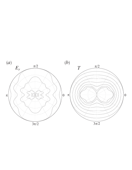
FIG. 2.: $M_{f}(\theta)$ in a trap with $E_{R}=25\hbar\omega$ and $\lambda=11$, for $(a)$ $T=0$, for $E_{F}/(\hbar\omega)$ ranging from $1$ (outermost) to $45$ (innermost) in increments of 11; and $(b)$ $E_{F}=45\hbar\omega$ for $T/(\hbar\omega)$ ranging from 0.5 (innermost) to 3.5 (outermost) in increments of 0.5. The radial scale is linear, and the same for all curves; the radius of the circular frames is one.

The results of evaluating numerically Eq. (6) are displayed in Fig. 2. Examining these results reveals, in addition to fine structure for which no simple, qualitative explanation is apparent, a rather surprising general feature. As $E_{F}$ rises from zero, Fermi inhibition is initially strongest in the direction in which the trap is stiffer; but at high $E_{F}$, it is emission in the soft direction which is most inhibited. One might think to explain the greater initial inhibition in the stiff direction by reference to the lower density of states into which the emitting atom must recoil, if it recoils in the stiff direction. This tempting explanation is incorrect, however, because the larger trap force in the stiff direction allows greater violation of momentum conservation, and consequently the range of energy levels into which the atom may recoil is also greater. It is actually trivial to show that the greater width of $|\langle n|e^{ik\hat{x}}|m\rangle|^{2}$ exactly compensates for the lower density of states, if all final states $|n\rangle$ are available (which is why emission by a single atom is independent of the trap shape). And this reveals the true explanation for the crossover from soft to stiff directions. While $|\langle n|e^{ik\hat{x}}|m\rangle|^{2}$ is peaked at the same energy $E_{R}$ regardless of $\lambda$, the wider distribution for the stiff direction is first to be encroached on by the rising Fermi level, which prevents recoil into occupied states. The wider distribution is also last to be completely submerged as $E_{F}$ rises past $E_{R}$, so for large $E_{F}$ spontaneous emission is preferentially in the stiff direction. And the crossover point is once again $E_{F}=E_{R}$.

While Fig. 2 presents results for a prolate (‘cigar-shaped’) trap, so that ‘the soft direction’ is actually the equatorial plane, to describe an oblate (‘pancake-shaped’) trap one need merely rotate the circular plots by ninety degrees. One piece of curious structure in $M_{f}(\theta)$ as a function of $E_{F}$ which is not shown in Fig. 2(a) is that if $\lambda$ is an integer, $M_{f}(0)$ and $M_{f}(\pi)$ are $\lambda$-fold degenerate as functions of integer $E_{F}/(\hbar\omega)$. If $\lambda$ is the inverse of an integer, $M_{f}(\pm\pi/2)$ are similarly degenerate. Fig. 2(b) shows that at finite temperatures $M_{f}(\theta)$ becomes more isotropic. Indeed, at very high temperature complete isotropy is restored, as Pauli exclusion becomes insignificant in the classical limit. Therefore the occurrence of the spatial anisotropy of the spectrum can also be used signaling the onset of the degenerate regime in the cooling process of the gas.

So far we have assumed that the one excited atom had initially been brought into the trap without any disturbance of the equilibrium population of ground state atoms. But let us now consider the experimentally more straightforward scenario in which the excited atom has been created by applying a laser pulse to a ground state cloud. To ensure that no more than one excited atom is involved, we suppose a weak pulse. On the other hand, we will assume that the pulse is short compared to the internal and external dynamics of the atoms, so that we can consider it instantaneous. Taking the excited atom from the ground state cloud introduces two significant changes. Firstly, even at zero temperature there is a significant probability of the excited atom having energy above $E_{F}$, because it may have been excited from a motional state near the Fermi level. And secondly, the excitation of one atom leaves behind a hole in the Fermi sea, into which the atom can always recoil.

Recalculating the rate of spontaneous emission in an isotropic trap, from the initial state with one atom excited from the cloud as we have described, we obtain

$$\tilde{M_{f}}(\Omega)=1+\frac{1}{N}\left[|\sum_{\vec{l}}\langle n_{\vec{l}}\rangle C_{\vec{l}\vec{l}}(\Omega)|^{2}-\sum_{\vec{l}\vec{l}^{\prime}}\langle n_{\vec{l}}\rangle\langle n_{\vec{l}^{\prime}}\rangle|C_{\vec{l}\vec{l}^{\prime}}(\Omega)|^{2}\right]\;,$$ (7)

where $\tilde{M_{f}}(\Omega)=\Gamma(\Omega)/[N\Omega_{R}^{2}t_{0}^{2}\Gamma_{0}(\Omega)]$ is the emission rate in the direction $\Omega$ given that an atom has indeed been excited. $\Omega_{R}$ is the Rabi frequency and $t_{0}$ the duration of the applied laser pulse. The $C_{\vec{l}\vec{l}^{\prime}}(\Omega)$ are the transition matrix elements between the states $|\vec{l}^{\prime}\rangle$ and $|\vec{l}\rangle$. The direction $\Omega$ is specified by the polar an azimuthal angles $(\theta,\phi)$ with respect to the propagation direction of the exciting laser pulse. Obviously, the results for the isotropic trap depend only on $\theta$.

The first term within the large brackets in Eq. (7) represents processes in which an atom is excited by the laser pulse, then spontaneously emits a photon and recoils back into the ‘hole’ from which it came. Because the final state of the gas is the same no matter which atom undergoes this process, absorption and re-emission by all $N$ atoms interfere constructively, and so this term is of order $N^{2}$; but since the atom recoils back into the state from which it was kicked by the laser pulse, the re-emitted photon is overwhelmingly likely to be in the same direction as the pulse [6]. The second term in the brackets of Eq. (6) describes Fermi-inhibited spontaneous emission just as we have discussed in the first part of this Letter, but with the more complicated initial state for the excited atom. It is this term that is of interest, but since it is only proportional to $N$, it is dominated by the first term within a cone around the forward direction. Evaluating the two terms for small angles from the laser direction, one finds the width of this cone to be $|\delta\theta|\sim(\eta N^{1/6})^{-1}\sim 1/(k_{0}L)$, where $L$ denotes the atomic cloud size (see Fig. 3). This is the familiar results of diffraction of light by a transparent object of size $L$.

We have plotted in Fig. 3 $\tilde{M_{f}}(\theta)$ as function of $\theta$. For $\theta>\delta\theta$, Fermi inhibition is indeed significant, though it is nowhere close to the near-total suppression found in the cases where the excited atom is initially thermal. This is because there is always a significant fraction of the ground state atoms within two recoil energies of $E_{F}$, and these can be excited and spontaneously emit without much hindrance.

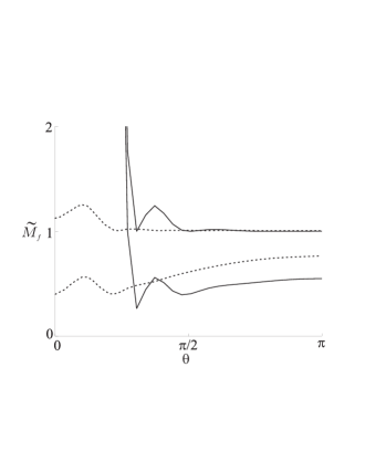
FIG. 3.: $\tilde{M_{f}}$ at $T=0$ for a trap with $E_{R}=\hbar\omega$ and $E_{F}=10\hbar\omega$. The solid line corresponds to Eq. 7 and the dashed line to the case where forward scattering is suppressed by a Raman pulse excitation. In both cases the above lying curve is missing the Fermi-inhibition term (the last one in Eq. 7).

To see Fermi inhibition without simply waiting for rare emissions outside the forward cone, one possibility is to make the exciting pulse a Raman pulse, so that the recoil momentum when the atom emits one photon is different from its recoil on absorbing the two Raman photons. By this means one can ensure that recoil back into the hole the excited atom came from is strongly suppressed by momentum conservation, and the order $N^{2}$ term in Eq. (6) can be essentially eliminated. This effect is shown by the dotted curves in Fig. 3. We emphasize, however, that the Raman laser should involve a dipole forbidden transition in order for the $|e\rangle\to|g\rangle$ to be allowed, which makes the experiment more challenging.

Finally, we would like to mention that in the calculations presented here we have neglected atom–atom collisions, which is a good approximation since s–wave scattering is suppressed for spin polarized Fermions. On the other hand, Fermi’s golden rule neglects the effects of dipole–dipole interactions and reabsorption, and therefore our model assumes that the atomic gas is optically thin, meaning that the probability of reabsorbtion of the emitted photon $P_{reab}=\frac{\sigma_{E}}{4\pi}\langle\frac{1}{r_{12}^{2}}\rangle$ [7] is negligible. Some straightforward calculations show that this implies the condition $0.15E_{f}^{2}/(E_{R}\hbar\omega)\ll 1$, which for stiff traps will still allow significant Fermi inhibition.

In conclusion, we have analyzed the possibility of observing Fermi inhibition of spontaneous emission in an atomic gas. We have derived simple analytical formulas for the modification factor $M_{f}$ and compared with numerical results for both isotropic and cylindrically symmetric traps. We have also studied the situation in which an atom is excited by a weak short laser.

This work was supported by the European Union under the TMR Network ERBFMRX-CT96-0002 and by the Austrian Fond zur Förderung der wissenschaftlichen Forschung. We thank W. Ketterle for pointing us out that Fermi inhibition was already predicted in [8].

REFERENCES

- [1] E. M. Purcell, Phys. Rev. 69, 681 (1946)
- [2] D. Kleppner, Phys. Rev. Lett. 47, 233 (1981)
- [3] For recent work on trapped Fermi gases see for example: D. A. Butts and D. S. Rokhsar, Phys. Rev. A 55, 4346 (1997); J. Schneider and H. Wallis, Phys. Rev. A 57, 1253 (1998); F. Brosens, J. T. Devreese, and L. F. Lemmens, cond-mat/9710126; M. Houbiers, R. Ferwerda, H.T.C. Stoof, W.I. McAlexander, C.A. Sackett, and R.G. Hulet, Phys. Rev A 56, 4846 (1997); M. A. Baranov, Yu. Kagan, and M. Yu. Kagan, JETP Letters 64, 301 (1996)
- [4] M. Abramowitz and I. A. Stegun, Handbook of Mathematical Functions (Dover Publications Inc. New York, 1972)
- [5] C. Cohen Tannoudji, J. Dupont-Roc, and G. Grynberg, Atom-Photon Interactions (John Wiley & Sons, Inc, 1992)
- [6] In the limit where the time-scale for this forward re-emission is as short as the laser pulse itself, it is of course necessary to re-interpret forward spontaneous emission as coherent forward scattering. Re-summing these terms to all orders would then reveal how the propagation of the pulse through the cloud is modified by the index of refraction of the gas. But we will assume that the pulse is so short compared to that we are far from this limit.
- [7] Y. Castin, J.I. Cirac, and M. Lewenstein, submitted
- [8] K. Helmerson, M. Xiao, and D. Pritchard, IQEC’90 book of abstracts, QTHH4