Finite Temperature Perturbation Theory for a Spatially Inhomogeneous Bose-condensed Gas

Abstract

We develop a finite temperature perturbation theory (beyond the mean field) for a Bose-condensed gas and calculate temperature-dependent damping rates and energy shifts for Bogolyubov excitations of any energy. The theory is generalized for the case of excitations in a spatially inhomogeneous (trapped) Bose-condensed gas, where we emphasize the principal importance of inhomogeneity of the condensate density profile and develop the method of calculating the self-energy functions. The use of the theory is demonstrated by calculating the damping rates and energy shifts of low-energy quasiclassical excitations, i.e. the quasiclassical excitations with energies much smaller than the mean field interaction between particles. In this case the boundary region of the condensate plays a crucial role, and the result for the damping rates and energy shifts is completely different from that in spatially homogeneous gases. We also analyze the frequency shifts and damping of sound waves in cylindrical Bose condensates and discuss the role of damping in the recent MIT experiment on the sound propagation.

I Introduction

Recent developments in the physics of ultra-cold gases have led to the discovery of Bose-Einstein condensation (BEC) in trapped clouds of alkali atoms [1, 2, 3] and stimulated a tremendous boost in theoretical studies of weakly interacting Bose gases. As in previous years, these studies rely on the binary approximation for the interparticle interaction. The latter is characterized by the 2-body scattering length $a$, which assumes the presence of a small gaseous parameter $na^{3}\ll 1$ (n is the gas density). Especially intensive are the attempts to reach beyond the ordinary mean field approach and to develop a theory which can properly describe the behavior of finite temperature elementary excitations of a trapped Bose-condensed gas and in particular, explain the JILA [4] and MIT [5] experiments on energy shifts and damping rates of the excitations.

The commonly used mean field theory (for $a>0$) is based on the Bogolyubov quasiparticle approach developed originally for a spatially homogeneous Bose-condensed gas at $T\rightarrow 0$ [6] and employed by Lee and Yang [7] (see also [8]) at finite temperatures. The generalization of the Bogolyubov method for spatially inhomogeneous systems has been described by De Gennes [9]. In the case of a Bose-condensed gas it should be completed by the equation for the wavefunction of the spatially inhomogeneous condensate, derived by Pitaevskii [10] and Gross [11].

For spatially homogeneous gases the theory beyond the mean field approach was also developed. Beliaev [12] constructed the zero-temperature diagram technique which allows one to find corrections to the energies of Bogolyubov excitations, proportional to $(n_{0}a^{3})^{1/2}$, where $n_{0}$ is the condensate density. The corrections are provided by the interaction between the excitations (in particular, through the condensate) and contain both real (energy shift) and imaginary (damping rate) parts. At $T=0$ the latter originates from spontaneous decay of a given excitation ($\nu$) to two other excitations ($\gamma$ and $\gamma^{\prime}$), with smaller energies and momenta: $\nu\rightarrow\gamma+\gamma^{\prime}$. A universal expression for the chemical potential in terms of the self-energy functions has been found by Pines and Hugenholtz [13]. It should be emphasized that the corrections proportional to $n_{0}a^{3}$ already depend on the contribution of 3-body interactions and, hence, can not be obtained within the binary approximation.

The Beliaev approach was employed by Popov [14] at finite temperatures. In this case the corrections to the Beliaev self-energies contain infra-red singularities, i.e. they tend to infinity for momenta $p\rightarrow 0$. This prompted Popov to make a renormalization of the theory, which links the microscopic approach with phenomenological Landau hydrodynamics [15]. The Popov theory eliminates the infra-red singularities and allows one to describe the behavior of low-energy excitations (phonons) at temperatures much smaller than the mean field interparticle interaction $n_{0}\tilde{U}$ ($\tilde{U}=4\pi\hbar^{2}a/m$, with $m$ being the atom mass). The damping of phonons in this temperature range is determined by the Beliaev damping processes and has also been calculated by Hohenberg and Martin [16]. A simplified approach within the dielectric formalism was used by Szepfalusy and Kondor [17] for calculating the damping rates of excitations in the phonon branch of the spectrum. They found that at temperatures $T\gg n_{0}\tilde{U}$ the damping rate of a given excitation ($\nu$) originates from the scattering of thermal excitations ($\gamma$ and $\gamma^{\prime}$) on the excitation $\nu$ through the processes $\nu+\gamma\leftrightarrow\gamma^{\prime}$. Since the characteristic energies of the thermal excitations $\gamma$, $\gamma^{\prime}$ turn out to be much larger than the energy of the excitation $\nu$, this damping channel can be treated as Landau damping. It should be noted that the damping rates can be simply found by considering the interaction between the excitations as a small perturbation and using Fermi’s golden rule. This allows one to properly take into account the Bogolyubov nature of the thermal excitations. The damping rates of phonons in a spatially homogeneous Bose-condensed gas, in particular for the Szepfalusy-Kondor mechanism, have been calculated in the recent contributions [18, 19, 20, 21, 22].

In order to reach beyond the mean field theory at $T\gtrsim n_{0}\tilde{U}$ one should further develop the Popov approach. One can also proceed along the lines of the Beliaev theory, since any physical quantity should be determined by combinations of the Beliaev self-energies, which do not contain the infrared singularities. In this paper we choose the latter way and construct the perturbation theory for a Bose-condensed gas, which allows us to find the next to leading order terms (the terms proportional to $(n_{0}a^{3})^{1/2}$) in the energy spectrum of the elementary excitations. As in [17, 18, 19, 20, 21, 22], we consider the excitations in the so-called collisionless regime, where their De Broglie wavelength is much smaller than the mean free path of the thermal excitations.

We start with the case of a spatially homogeneous Bose-condensed gas and find temperature-dependent energy shifts and damping rates for Bogolyubov excitations of any energy. At temperatures $T\gg n_{0}\tilde{U}$ the small parameter of the theory proves to be

$$\frac{T}{n_{0}\tilde{U}}(n_{0}a^{3})^{1/2}\ll 1,$$ (1)

in contrast to $n_{0}a^{3}\ll 1$ for $T=0$. The appearance of the extra factor ($T/n_{0}\tilde{U}$) originates from the Bose occupation numbers of thermal excitations with energies of order $n_{0}\tilde{U}$, which are the most important in the perturbation theory. As shown below, the damping of excitations with energies $\varepsilon_{\nu}\sim n_{0}\tilde{U}$ is determined by both the Szepfalusy-Kondor ($\nu+\gamma\leftrightarrow\gamma^{\prime}$) and Beliaev ($\nu\leftrightarrow\gamma+\gamma^{\prime}$) processes, and can no longer be treated as Landau damping.

The theory is generalized for the case of excitations in a spatially inhomogeneous (trapped) Bose-condensed gas. A new ingredient here is related to the inhomogeneous density profile of the condensate and the discrete structure of the excitation spectrum. We develop the method of calculating the self-energy functions and derive the equations for finding the wavefunctions and energies of the excitations (generalized Bogolyubov-De Gennes equations).

The use of the theory is demonstrated by two examples. The first one concerns quasiclassical low-energy excitations of a trapped Bose-condensed gas in the Thomas-Fermi regime. The term ”low-energy” assumes that the excitation energy $\varepsilon_{\nu}$ is much smaller than the mean field interparticle interaction $n_{0m}\widetilde{U}$ ($n_{0m}$ is the maximum condensate density), and the quasiclassical character of the excitations requires the condition $\varepsilon_{\nu}\gg\hbar\omega$, where $\omega$ is the characteristic trap frequency. We consider anisotropic harmonic traps, where the discrete structure of the excitation spectrum is not important (see below and in [21]). On the contrary, the inhomogeneity of the condensate density profile has a crucial consequence for the damping rates and energy shifts of quasiclassical low-energy excitations. The most important turns out to be the boundary region of the condensate, where $n_{0}({\bf r})\tilde{U}\sim\varepsilon_{\nu}$ [21]. Therefore, the result for the damping rates and energy shifts is completely different from that in spatially homogeneous gases.

Finally, we analyze the frequency shifts and damping of axially propagating sound waves in cylindrical Bose condensates. As found, the nature of damping is similar to that in the case of phonons in spatially homogeneous Bose condensates. We show that the attenuation of axially propagating sound wave packets in the recent MIT experiment [23] can be well explained as a consequence of this damping.

II General equations

We consider a weakly interacting Bose-condensed gas confined in an external potential $V({\bf r})$. The grand canonical Hamiltonian of the gas can be written as $\hat{H}=\hat{H}_{0}+\hat{H}_{1\text{ }}$, where (hereinafter $m=\hbar=1$)

$$\hat{H}_{0}=\int d^{3}r\hat{\Psi}^{\dagger}({\bf r})\left(-\frac{\Delta}{2}+V({\bf r})-\mu\right)\hat{\Psi}({\bf r}),$$ (2)

and the term

$$\hat{H}_{1}=\frac{\widetilde{U}}{2}\int d^{3}r\hat{\Psi}^{\dagger}({\bf r})\hat{\Psi}^{\dagger}({\bf r})\hat{\Psi}({\bf r})\hat{\Psi}({\bf r}),$$ (3)

assumes a point interaction between atoms. The field operator of atoms $\hat{\Psi}({\bf r})$ can be represented as the sum of the above-condensate part $\hat{\Psi}^{\prime}$ and the condensate wavefunction $\Psi_{0}\!=\!\langle\hat{\Psi}\rangle$ which is a c-number. As the interparticle interaction $\hat{H}_{1}$ contains both terms conserving the number of above-condensate particles and terms transferring two above-condensate particles to the condensate (or two condensate particles to the above-condensate part), the diagram technique should include both the normal Green function ${\cal G}$ and the anomalous Green function ${\cal F}$ (see, e.g. [12]).

FIG. 1.: The set of diagrams contributing to the normal self-energy $\Sigma$. Here a solid line with an arrow represents the normal Green function ${\cal G}$, solid line without an arrow corresponds to the anomalous Green function ${\cal F}$, white circle stands for the interaction vertex $\tilde{U}$ and the black circle represents a sum of two white circles, one being a direct interaction and the other an exchange interaction. Dashed lines stand for the condensate wave function $\sqrt{n_{0}}$. The self-energy part $\Sigma^{+}$ can be obtained by a time-reversal(i.e. the change $t\rightarrow-t$ and ${\bf p}\rightarrow-{\bf p}$) of the graphs shown above.

FIG. 2.: The set of graphs contributing to the anomalous self-energy $\Sigma_{a}$. The notations are the same as for the Fig.1.

The sums of the contributions of all irreducible diagrams will be represented by the normal ($\Sigma$) and anomalous ($\Sigma_{a}$) self-energies (see Fig.1 and Fig.2). The former corresponds to the processes conserving the number of above-condensate particles, and the latter describes absorption (or emission) of two particles to (out of) the condensate. The Green function and self-energy operators satisfy Beliaev-Dyson equations [12, 14]

$${\cal\,G} = G+G\Sigma{\cal G}+G\Sigma_{a}{\cal F},$$ (4)

$${\cal F} = G^{+}\Sigma^{+}{\cal F}+G^{+}\Sigma_{a}{\cal G},$$ (5)

where the Green functions $G$ and $G^{+}$ describe forward and backward propagation of a particle characterized by the Hamiltonian $\hat{H}_{0}$.

We confine ourselves to the case of repulsive interaction between the atoms ($a>0$). To develop the finite temperature perturbation theory for calculating dynamic properties and finding the excitation spectrum of a weakly interacting Bose-condensed gas we will use the non-equilibrium generalization [24] of the Matsubara diagram technique. In Eqs. (4),(5) we perform an analytical continuation of the Matsubara frequencies $\zeta_{j}=2\pi Tj$ ($j$ is an integer number) to the upper half-plane, which corresponds to the replacement $i\zeta_{j}\rightarrow\varepsilon+i0$. Then, multiplying both sides of Eqs. (4) and (5) by $G^{-1}$ and $(G^{+})^{-1}$, respectively, we arrive at the system of equations in the frequency-coordinate representation:

$$\varepsilon{\cal G}(\varepsilon;{\bf r},{\bf r}^{\prime}) = \left[-\frac{\Delta}{2}+V({\bf r})-\mu+\Sigma(\varepsilon)\right]{\cal G}(\varepsilon;{\bf r},{\bf r}^{\prime})+\Sigma_{a}(\varepsilon){\cal F}(\varepsilon;{\bf r},{\bf r}^{\prime})+\delta({\bf r}-{\bf r}^{\prime}),$$ (6)

$$-\varepsilon{\cal F}(\varepsilon;{\bf r},{\bf r}^{\prime}) = \left[-\frac{\Delta}{2}+V({\bf r})-\mu+\Sigma^{+}(\varepsilon)\right]{\cal F}(\varepsilon;{\bf r},{\bf r}^{\prime})+\Sigma_{a}(\varepsilon){\cal G}(\varepsilon;{\bf r},{\bf r}^{\prime}).$$ (7)

Here the action of the integral self-energy operators on the Green functions is written in a compact form $\int d^{3}r^{\prime\prime}\Sigma(\varepsilon;{\bf r},{\bf r}^{\prime\prime}){\cal G}(\varepsilon;{\bf r}^{\prime\prime},{\bf r}^{\prime})\equiv\Sigma(\varepsilon){\cal G}(\varepsilon;{\bf r},{\bf r}^{\prime})$ (and similar relations for the other combinations). Eqs. (6),(7) should be completed by a generalized Gross-Pitaevskii equation for the condensate wavefunction:

$$\left[-\frac{\Delta}{2}+V({\bf r})-\mu+(\Sigma-\Sigma_{a})|_{\varepsilon\rightarrow 0}\right]\Psi_{0}({\bf r})=0$$ (8)

and by the normalization condition

$\displaystyle\int d^{3}r\left(n_{0}({\bf r})+n^{\prime}({\bf r})\right)=N,$where $n_{0}({\bf r})=|\Psi_{0}({\bf r})|^{2}$ is the condensate density, $n^{\prime}({\bf r})=\left\langle\Psi^{\prime\dagger}({\bf r})\Psi^{\prime}({\bf r})\right\rangle$ is the density of above-condensate particles, and $N$ the total number of particles in the gas.

Eqs. (6),(7) can be solved by using the Bogolyubov transformation for the Green functions:

$${\cal G}(\varepsilon_{\nu};{\bf r},{\bf r}^{\prime}) = u_{\nu}({\bf r})u_{\nu}^{*}({\bf r}^{\prime})+v_{\nu}({\bf r})v_{\nu}^{*}({\bf r}^{\prime}),$$ (9)

$${\cal F}(\varepsilon_{\nu};{\bf r},{\bf r}^{\prime}) = -u_{\nu}({\bf r})v_{\nu}^{*}({\bf r}^{\prime})-v_{\nu}({\bf r})u_{\nu}^{*}({\bf r}^{\prime}),$$ (10)

where the index $\nu$ stands for the set of quantum numbers, and the functions $u_{\nu}$, $v_{\nu}$ satisfy generalized Bogolyubov-De Gennes equations

$$\varepsilon_{\nu}u_{\nu}({\bf r})\! \!=\! \!\left[\!-\frac{\Delta}{2}\!+\!V({\bf r})\!-\!\mu\!+\!\!\Sigma(\!\varepsilon_{\nu}\!)\!\right]\!\!u_{\nu}({\bf r})\!-\!\!\Sigma_{a}(\!\varepsilon_{\nu}\!)v_{\nu}({\bf r}),\!\!\!$$ (11)

$$\!-\varepsilon_{\nu}v_{\nu}({\bf r})\! \!=\! \!\left[\!-\frac{\Delta}{2}\!+\!V({\bf r})\!-\!\mu\!+\!\!\Sigma^{+}\!(\!\varepsilon_{\nu}\!)\!\right]\!\!v_{\nu}({\bf r})\!-\!\!\Sigma_{a}(\!\varepsilon_{\nu}\!)u_{\nu}({\bf r}).\!\!\!$$ (12)

In the Bogolyubov-De Gennes approach only the terms bilinear in $\widehat{\Psi}^{\prime}$ operators are retained in the interaction Hamiltonian $\hat{H}_{1}$, which assumes that the condensate density is much larger than the density of above-condensate particles. Then, the self-energy operators take the form

$$\Sigma(\varepsilon,{\bf r},{\bf r}^{\prime}) = 2n_{0}\widetilde{U}\delta({\bf r}-{\bf r}^{\prime}),$$ (13)

$$\Sigma_{a}(\varepsilon,{\bf r},{\bf r}^{\prime}) = n_{0}\widetilde{U}\delta({\bf r}-{\bf r}^{\prime}).$$ (14)

The result of their action on the condensate wavefunction $\Psi_{0}({\bf r})$ and the functions $u_{\nu}({\bf r})$, $v_{\nu}({\bf r})$ is reduced to

$\displaystyle\Sigma(\varepsilon_{\nu})\Psi_{0}({\bf r})=\int d^{3}r^{\prime}\Sigma(\varepsilon_{\nu},{\bf r},{\bf r}^{\prime})\Psi_{0}({\bf r}^{\prime})=2n_{0}({\bf r})\widetilde{U}\Psi_{0}({\bf r})$and similar relations for the other combinations. Then, Eq.(8) becomes the ordinary Gross-Pitaevskii equation

$$\left[-\frac{\Delta}{2}+V({\bf r})-\mu+n_{0}({\bf r})\widetilde{U}\right]\Psi_{0}({\bf r})=0,$$ (15)

and Eqs. (6),(7) are transformed to the ordinary Bogolyubov-De Gennes equations

$$\varepsilon_{\nu}u_{\nu}({\bf r}) = \left[-\frac{\Delta}{2}+V({\bf r})-\mu+2n_{0}({\bf r})\widetilde{U}\right]u_{\nu}({\bf r})-n_{0}({\bf r})\widetilde{U}v_{\nu}({\bf r}),$$ (16)

$$-\varepsilon_{\nu}v_{\nu}({\bf r}) = \left[-\frac{\Delta}{2}+V({\bf r})-\mu+2n_{0}({\bf r})\widetilde{U}\right]v_{\nu}({\bf r})-n_{0}({\bf r})\widetilde{U}u_{\nu}({\bf r}).$$ (17)

Taking into account Eq.(15), in terms of the functions $f_{\nu}^{\pm}=u_{\nu}\pm v_{\nu}$ these equations can be rewritten as

$$\varepsilon_{\nu}f^{-}_{\nu}({\bf r}) = \left(-\frac{\Delta}{2}+\frac{\Delta\Psi_{0}}{2\Psi_{0}}\right)f^{+}_{\nu}({\bf r})$$ (18)

$$\varepsilon_{\nu}f^{+}_{\nu}({\bf r}) = \left(-\frac{\Delta}{2}+\frac{\Delta\Psi_{0}}{2\Psi_{0}}+2|\Psi_{0}|^{2}\widetilde{U}\right)f^{-}_{\nu}({\bf r}).$$ (19)

For a trapped Bose-condensed gas in the Thomas-Fermi regime, where $\mu\approx n_{0\max}\widetilde{U}$ is much larger then the spacing between the trap levels, the kinetic energy term in Eq. (15) can be omitted and one has [25]

$$\Psi_{0}=\sqrt{\frac{\mu-V({\bf r})}{\widetilde{U}}},$$ (20)

if the argument of the square root is positive and zero otherwise. For the low-energy excitations ($\varepsilon_{\nu}\ll n_{0m}\widetilde{U}$) of Thomas-Fermi condensates Eqs. (18),(19) can be reduced to hydrodynamic equations obtained by Stringari [26] and solved in the case of spherically symmetric harmonic potential $V(r)$ and for some excitations in a cylindrically symmetric potential. An analytical method of solving Eqs. (18),(19) (or the corresponding hydrodynamic equations) for the low-energy excitations of Thomas-Fermi condensates in an anisotropic harmonic potential $V({\bf r})$ has been developed in [27, 28].

For a spatially homogeneous gas the generalized Gross-Pitaevskii equation (8) is equivalent to the Pines-Hugenholtz identity [13]. In the Bogolyubov approach it simply gives $\mu=n_{0}\widetilde{U}$, and Eqs. (16),(17) lead to the Bogolyubov spectrum

$$\varepsilon_{p}=\sqrt{(p^{2}/2)^{2}+n_{0}\widetilde{U}p^{2}},$$ (21)

where ${\bf p}$ is the momentum of the excitation.

Under the condition $n_{0}\gg n^{\prime}$, for which the Bogolyubov approach was originally developed, one can simply put $n_{0}$ equal to the total density $n$ in Eq.(21). For $n^{\prime}\gtrsim n_{0}$, which can be the case at $T\gg\mu$, the dispersion law becomes essentially temperature dependent [7, 8]. In a spatially homogeneous gas the temperature dependence predominantly originates just from the presence of above condensate particles, with $n^{\prime}\approx n(T/T_{c})^{3/2}$ where $T_{c}=3.31n^{2/3}$ is the BEC transition temperature. This leads to the replacement $n_{0}\rightarrow n_{0}+n^{\prime}$ in Eq.(13) and gives $\mu=(n_{0}+2n^{\prime})\widetilde{U}$. The dispersion law will be still given by Eq.(21) in which the condensate density is now temperature dependent: $n_{0}=n\left[1-(T/T_{c})^{3/2}\right]$.

III Spatially homogeneous Bose-condensed gas

In this section we present the results for the damping rates and energy shifts of elementary excitations in an infinitely large spatially homogeneous Bose-condensed gas. As one can see from Eqs.(16),(17), for finding the energy spectrum and wavefunctions of the excitations it is sufficient to calculate the self-energies $\Sigma$, $\Sigma^{+}$ and $\Sigma_{a}$. We will perform the calculations in the frequency-momentum representation and for physical transparency consider temperatures

$$T\gg n_{0}\tilde{U}$$ (22)

(the opposite limiting case has been discussed by Popov [14] with regard to the phonon branch of the excitation spectrum). In the zero order approximation in the parameter $\left(n_{0}a^{3}\right)^{1/2}$ we have the well-known mean field result: $\Sigma^{(0)}=\Sigma^{(0)+}=2(n_{0}+n^{\prime(0)})\widetilde{U}$, $\Sigma_{a}^{(0)}=n_{0}\widetilde{U}$, with $n^{\prime(0)}=n(T/T_{c})^{3/2}$ (see above). In this approach we obtain the Bogolyubov quasiparticle excitations with the spectrum (21), which we use in order to calculate the next order in $\left(n_{0}a^{3}\right)^{1/2}$. The latter is determined by the contribution of diagrams containing one quasiparticle loop [14] (see Figures 1 and 2). Actually in this approach we represent the Hamiltonian as the sum of the (diagonalized) Bogolyubov Hamiltonian and the perturbation $\widehat{H}_{{\rm int}}$ originating from $\widehat{H}_{1}$ (3) and containing the terms proportional to $\Psi_{0}\hat{\Psi}^{\prime 3}$ and $\hat{\Psi}^{\prime 4}$:

$$\hat{H}_{{\rm int}}=\tilde{U}\int d^{3}r[\Psi_{0}({\bf r})\hat{\Psi}^{\prime\dagger}({\bf r})\{\hat{\Psi}^{\prime\dagger}({\bf r})+\hat{\Psi}^{\prime}({\bf r})\}\hat{\Psi}^{\prime}({\bf r})+(1/2)\hat{\Psi}^{\prime\dagger}({\bf r})\hat{\Psi}^{\prime\dagger}({\bf r})\hat{\Psi}^{\prime}({\bf r})\hat{\Psi}^{\prime}({\bf r})].$$ (23)

Retaining only the temperature-dependent contributions, after laborious calculations for the normal self-energy we obtain $\Sigma=\Sigma^{(0)}+\Sigma^{(1)}$, where

$$\Sigma^{(1)}(P) =\Sigma^{n}(P)+\Sigma^{r}(P),$$ (24)

$$\Sigma^{n}(P) =2\widetilde{U}^{2}n_{0}\int\frac{d^{3}q}{(2\pi)^{3}}(n_{q}+n_{k})\left(\frac{2A_{k}B_{q}+A_{q}A_{k}-4A_{k}C_{q}+2C_{q}C_{k}}{\varepsilon-\varepsilon_{q}-\varepsilon_{k}}-\right.$$ (26)

$$\left.\frac{2A_{q}B_{k}+B_{q}B_{k}-4B_{k}C_{q}+2C_{q}C_{k}}{\varepsilon+\varepsilon_{k}+\varepsilon_{q}}\right)-8(\pi n_{0}a^{3})^{1/2}T,$$

$$\Sigma^{r}(\!P)\!\! =2\widetilde{U}^{\!2}\!n_{\!0}\!\!\int\!\!\!\frac{d^{3}q}{(2\pi)^{3}}\!\frac{\!n_{\!q}\!-\!n_{\!k}}{\varepsilon\!+\!\varepsilon_{\!q}\!-\!\varepsilon_{\!k}}(2A_{q}A_{k}\!+\!2A_{k}B_{q}\!+\!2B_{k}B_{q}\!+\!4C_{k}C_{q}\!-\!4A_{k}C_{q}\!-\!4B_{q}C_{k}).$$ (27)

Here $P=\{\varepsilon,{\bf p}\}$, ${\bf k}={\bf q}+{\bf p}$, $E_{p}=p^{2}/2$, $\varepsilon_{p}$ is given by Eq.(21), $n_{q}$ is the equilibrium occupation number, $C_{p}=n_{0}\widetilde{U}/2\varepsilon_{p}$ and $A_{p},B_{p}=(\pm\varepsilon_{p}+E_{p}+n_{0}\widetilde{U})/2\varepsilon_{p}$. Similarly, the correction to the anomalous self-energy is given by

$$\Sigma_{a}^{(1)}(P) = \Sigma_{a}^{n}(P)+\Sigma_{a}^{r}(P),$$ (28)

$$\Sigma_{a}^{n}(P) = 2\widetilde{U}^{2}n_{0}\int\frac{d^{3}q}{(2\pi)^{3}}(n_{k}+n_{q})\left(\frac{2A_{k}B_{q}-2A_{k}C_{q}-2B_{q}C_{k}+3C_{q}C_{k}}{\varepsilon-\varepsilon_{q}-\varepsilon_{k}}-\right.$$ (30)

$$\left.\frac{2A_{q}B_{k}-2B_{k}C_{q}-2A_{q}C_{k}+3C_{k}C_{q}}{\varepsilon+\varepsilon_{k}+\varepsilon_{q}}\right)-4(\pi n_{0}a^{3})^{1/2}T,$$

$$\Sigma_{a}^{r}(P)\! =\!\! \!2\widetilde{U}^{2}n_{0}\int\!\!\!\frac{d^{3}q}{(2\pi)^{3}}\frac{n_{q}-n_{k}}{\varepsilon+\varepsilon_{q}-\varepsilon_{k}}(2A_{\!k}A_{\!q}\!+\!2B_{\!k}B_{\!q}\!+\!6C_{\!k}C_{\!q}\!-\!2A_{\!k}C_{\!q}\!-\!2A_{\!q}C_{\!k}\!-\!2B_{\!q}C_{\!k}\!-\!2B_{\!k}C_{\!q}).$$ (31)

The resonant parts $\Sigma^{r},\Sigma_{a}^{r}$ originate from the terms where one of the intermediate quasiparticles is created and another one annihilated, and the non-resonant parts $\Sigma^{n},\Sigma_{a}^{n}$ from the terms where both intermediate quasiparticles are created (annihilated). Temperature independent terms in the non-resonant parts, found by Beliaev [12], are omitted in Eqs.(26)-(31).

Each of the self-energies (26)-(31) is singular at $P\rightarrow 0$ and at least for small momenta the corrections become larger than the mean field values (13). Nevertheless, keeping in mind that any physical quantity is determined by the combinations of the self-energies, which do not contain the infra-red singularities, we will still treat $\Sigma^{(1)}$ and $\Sigma_{a}^{(1)}$ as perturbations.

For a spatially homogeneous gas the Pines-Hugenholtz identity $\mu=(\Sigma(P)-\Sigma_{a}(P))|_{P\rightarrow 0}$ gives the first order correction to the chemical potential

$$\mu^{(1)}=-\beta\sqrt{n_{0}};\,\,\,\,\,\,\beta=12(\pi a^{3})^{1/2}T,$$ (32)

and the relation between $n_{0}$ and the chemical potential, $\mu=n_{0}\widetilde{U}-\beta\sqrt{n_{0}}$, coincides with that found by Popov [14]. The $u,v$ functions in generalized Bogolyubov-De Gennes equations (11), (12) can be written as $u_{p}\exp(i{\bf pr})$ and $v_{p}\exp(i{\bf pr})$, and in terms of the functions $f^{\pm}_{p}=u_{p}\pm v_{p}$ these equations take the form

$$(\varepsilon-S^{-}(P))f^{-}_{p} = \left(\frac{p^{2}}{2}+S^{+}_{-}(P)\right)f^{+}_{p},$$ (33)

$$(\varepsilon-S^{-}(P))f^{+}_{p} = \left(\frac{p^{2}}{2}+2n_{0}\widetilde{U}+S^{+}_{+}(P)\right)f^{-}_{p},$$ (34)

where

$$S^{+}_{\pm} = \frac{\Sigma^{(1)}+\Sigma^{+(1)}}{2}+\beta\sqrt{n_{0}}\pm\Sigma_{a},$$ (35)

$$S^{-} = \frac{\Sigma^{(1)}-\Sigma^{+(1)}}{2}.$$ (36)

Considering the terms $S^{-}$, $S^{+}_{\pm}$ in Eqs. (33),(34) as small perturbations we put $\varepsilon=\varepsilon_{p}$ in the expressions for these quantities, following from Eqs. (26)-(31). Then, solving Eqs. (33),(34), for the excitation energy we obtain $\varepsilon=\varepsilon_{p}+\varepsilon_{p}^{(1)}$, where

$$\!\varepsilon_{p}^{(1)}\!\!=\!\!\left[\!\frac{E_{p}}{2\varepsilon_{p}}\!S^{+}_{+}(P)\!+\!\frac{\varepsilon_{p}}{2E_{p}}S^{+}_{-}(P)\!+\!S^{-}(P)\right]_{P\rightarrow(\varepsilon_{p},{\bf p})}\!,$$ (37)

As $\Sigma^{(1)}$ and $\Sigma_{a}^{(1)}$ are complex, the correction to the excitation energy has both a real and an imaginary part: $\varepsilon_{p}^{(1)}=\delta\varepsilon_{p}-i\Gamma_{p}$. The former gives the energy shift, and the latter is responsible for damping of the excitations. Under the condition $T\gg n_{0}\widetilde{U}$ a straightforward calculation of Eq.(37) on the basis of Eqs. (26)-(31) and (35),(36), for the phonon branch of the spectrum ($\varepsilon_{p}\ll n_{0}\widetilde{U}$) yields

$$\delta\varepsilon_{p} \approx -7\varepsilon_{p}\frac{T}{n_{0}\widetilde{U}}(n_{0}a^{3})^{1/2},$$ (38)

$$\Gamma_{p} = \varepsilon_{p}\frac{3\pi^{3/2}T}{4n_{0}\widetilde{U}}(n_{0}a^{3})^{1/2}.$$ (39)

It is important to emphasize that in this case the energy shift is determined by both resonant and non-resonant terms, whereas the damping rate $\Gamma_{p}$ is described solely by the resonant contributions. This type of damping originates from quasi-resonant scattering of thermal excitations from a given excitation (Landau damping) and is absent at $T=0$. Both the energy shift and the damping rate are determined by the interaction of a given excitation with intermediate quasiparticles having energies $\varepsilon_{q}\sim n_{0}\widetilde{U}$. The damping rate $\Gamma_{p}$ (39) coincides with that found in recent contributions [18, 20, 21, 22] and contains a slight numerical difference from the earlier Szepfalusy-Kondor result [17]. The energy shift for the phonon branch of the spectrum was also calculated in [18]. In the latter work the expansion of the self-energy functions near the point $\varepsilon=\varepsilon_{p}$ was used and formally divergent integrals were canceling each other in the final expression for the energy shift, which have led to the result by approximately factor 6 smaller then the shift (38) obtained by the exact integration.

Eqs.(38),(39) clearly show that the small parameter of the theory is $(T/n_{0}\tilde{U})(n_{0}a^{3})^{1/2}\ll 1$ (see Eq.(1)), whereas in the zero temperature approach [12] the small parameter is $(n_{0}a^{3})^{1/2}\ll 1$. The presence of an additional large factor $T/n_{0}\widetilde{U}$ at finite temperatures $T\gg n_{0}\widetilde{U}$ originates from the Bose enhancement diagrams containing one quasiparticle loop: Compared to the zero-temperature case the contribution of each of these diagrams is multiplied by the Bose factor $n_{q}=[\exp{(\varepsilon_{q}/T)}-1]^{-1}$ (or $1+n_{q}$). As the most important is the contribution of intermediate quasiparticles with energies $\varepsilon_{q}\sim n_{0}\widetilde{U}$, for $T\gg n_{0}\widetilde{U}$ the Bose factor $n_{q}\sim T/n_{0}\widetilde{U}$. The criterion similar to Eq.(1) was found by Popov [8, 14] as the condition which allows one to use the mean field approach at finite temperatures and to renormalize the theory for reaching beyond this approach.

Remarkably, the criterion (1) is fulfilled even at temperatures very close to $T_{c}$. For $\Delta T=T_{c}-T\ll T_{c}$ we have $n_{0}\sim n\Delta T/T_{c}$, and Eq.(1) gives $\Delta T/T_{c}\gg(n_{0}a^{3})^{1/3}$, which coincides with the well known Ginzburg criterion [29] for the absence of critical fluctuations. The criterion (1) also ensures that the main contribution to the damping rate originates from the interaction of a given excitation with thermal excitations through the condensate, i.e., from the first term in $\hat{H}_{\rm int}$ (23).

At energies $\varepsilon_{p}\gtrsim n_{0}\widetilde{U}$ (but still $\varepsilon_{p}\ll T$) the results for the energy shift and damping rate, following from Eq.(37), can be represented in the form

$$\delta\varepsilon_{p} = \varepsilon_{p}F_{1}\left(\frac{\varepsilon_{p}}{n_{0}\widetilde{U}}\right)\frac{T}{n_{0}\widetilde{U}}(n_{0}a^{3})^{1/2},$$ (40)

$$\Gamma_{p} = \varepsilon_{p}F_{2}\left(\frac{\varepsilon_{p}}{n_{0}\widetilde{U}}\right)\frac{T}{n_{0}\widetilde{U}}(n_{0}a^{3})^{1/2}.$$ (41)

The functions $F_{1}$ and $F_{2}$ have been calculated numerically. For $\varepsilon_{p}\ll n_{0}\widetilde{U}$ we have $F_{1}\approx-7$, $F_{2}=3\pi^{3/2}/4$ and Eqs. (40), (41) coincide with Eqs. (38), (39). The dependence of $\delta\varepsilon_{p}$ and $\Gamma_{p}$ on the excitation energy is presented in Fig.3. For $\varepsilon_{p}\lesssim n_{0}\widetilde{U}$ the damping rate increases with $\varepsilon_{p}$ and reaches its maximum at $\varepsilon_{p}\sim 10n_{0}\widetilde{U}$. Further increase of $\varepsilon_{p}$ leads to slowly decreasing $\Gamma_{p}$. For single-particle excitations ($\varepsilon_{p}=p^{2}/2\gg n_{0}\widetilde{U}$) we obtain $F_{2}(\varepsilon_{p}/n_{0}\widetilde{U})\sim(n_{0}\widetilde{U}/\varepsilon_{p})^{3/2}$. Accordingly, the damping rate can be written as $\Gamma_{p}\sim(T/\varepsilon_{p})n_{0}\sigma v_{p}$, where $\sigma=8\pi a^{2}$ is the elastic cross section, and $v_{p}$ the particle velocity. This damping rate exceeds the Beliaev temperature-independent term $n\sigma v_{p}$ even at $T$ close to $T_{c}$, if $\Delta T=T_{c}-T\gg\varepsilon_{p}$. In contrast to the phonon branch of the spectrum, for $\varepsilon_{p}\gtrsim n_{0}\widetilde{U}$ the damping is provided by both the Szepfalusy-Kondor ($\nu+\gamma\leftrightarrow\gamma^{\prime}$) and Beliaev ($\nu\leftrightarrow\gamma+\gamma^{\prime}$) processes and, hence, can no longer be treated as Landau damping. The small parameter of the theory is still given by Eq.(1), since even at $\varepsilon_{p}\gg n_{0}\widetilde{U}$ the energy of at least one of the thermal excitations is of order $n_{0}\widetilde{U}$.

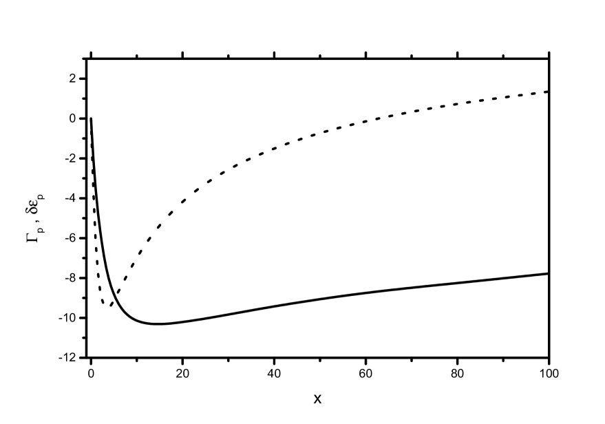
FIG. 3.: The damping rate $\Gamma_{p}$ (solid line) and the energy shift $\delta\varepsilon_{p}$ (dashed line) versus $(\varepsilon_{p}/n_{0}\widetilde{U})$. Both $\Gamma_{p}$ and $\delta\varepsilon_{p}$ are given in the units of $T(n_{0}a^{3})^{1/2}$.

The energy shift for $\varepsilon_{p}\lesssim n_{0}\widetilde{U}$ is negative. The modulus of the shift increases with $\varepsilon_{p}$ and reaches its maximum at $\varepsilon_{p}\approx 4n_{0}\widetilde{U}$. The further increase of $\varepsilon_{p}$ decreases $|\delta\varepsilon_{p}|$. The latter is equal to zero for $\varepsilon_{p}\approx 60n_{0}\widetilde{U}$, and becomes positive at larger $\varepsilon_{p}$.

The above results for the damping rate and energy shift of a given excitation are obtained in the so called collisionless regime: We assume that the De Broglie wavelength of the excitation, $1/p$, is much larger than the mean free path of the thermal quasiparticles with energies $\sim n_{0}\widetilde{U}$, which are mostly responsible for the damping and shifts. It is also assumed that the excitation energy $\varepsilon_{p}$ greatly exceeds the damping rate of these thermal excitations. The latter is of order $T(n_{0}a^{3})^{1/2}$ (see Fig.3), and for $\varepsilon_{p}\gtrsim n_{0}\widetilde{U}$ the two requirements of the collisionless regime are well satisfied under condition (1). In the phonon branch of the excitation spectrum ($\varepsilon_{p}\ll n_{0}\widetilde{U}$) these requirements are equivalent to each other, and the collisionless criterion can be simply written as

$$\varepsilon_{p}\gg T(n_{0}a^{3})^{1/2}.$$ (42)

As clearly seen, in the phonon branch one can always find excitations which do not satisfy Eq.(42) and, hence, require a hydrodynamic description with regard to their damping rates and energy shifts.

The collisionless criterion (42) provides an additional argument on support of the above used perturbative approach for solving Eqs. (33), (34). Under condition (42) the term $S^{-}\lesssim T(n_{0}a^{3})^{1/2}\ll\varepsilon_{p}$, the term $S^{+}_{-}\lesssim\varepsilon_{p}(T/n_{0}\widetilde{U})(n_{0}a^{3})^{1/2}\ll p^{2}$, and the term $S^{+}_{+}\lesssim(n_{0}\widetilde{U}/\varepsilon_{p})T(n_{0}a^{3})^{1/2}\ll n_{0}\widetilde{U}$.

The non-mean-field shift $\delta\varepsilon_{p}$ is actually the shift of the excitation energy $\varepsilon_{p}$ at a given condensate density $n_{0}$. On the other hand, $\varepsilon_{p}$ is determined by the Bogolyubov dispersion law (21), with the temperature-dependent condensate density $n_{0}(T)$, and, hence, is temperature-dependent by itself. Therefore, at a given $T$ one will also have the mean-field temperature-dependent energy shift $\delta\varepsilon_{p}^{\rm mf}=\varepsilon_{p}(T)-\varepsilon_{p}(0)$. As the condensate density decreases with increasing temperature, $\delta\varepsilon_{p}^{\rm mf}$ is always negative. For $T\gg n_{0}\widetilde{U}$ it greatly exceeds the above calculated shift $\delta\varepsilon_{p}$ at any $p$. The ratio $(\delta\varepsilon_{p}^{\rm mf}/\delta\varepsilon_{p})$ decreases with temperature, but even for $n^{\prime}\ll n_{0}$ one has

$$\delta\varepsilon_{p}^{\rm mf}=-\varepsilon_{p}(0)\frac{n^{\prime}(T)\widetilde{U}}{p^{2}/2+2n_{0}(0)\widetilde{U}},$$ (43)

and $(\delta\varepsilon_{p}^{\rm mf}/\delta\varepsilon_{p})\sim(T/n_{0}\widetilde{U})^{1/2}\gg 1$.

IV Spatially inhomogeneous Bose-condensed gas

We now generalize the above obtained results for the case of elementary excitations in a spatially inhomogeneous (trapped) Bose-condensed gas. As already mentioned in the introduction, a new ingredient here is related to the inhomogeneous density profile of the condensate and the discrete structure of the excitation spectrum. This requires us to develop a new method of calculating the self-energy functions in generalized Bogolyubov-De Gennes equations (11), (12). The self-energy operators in these equations are the sums of the zeroth and first order terms:

$$\Sigma_{a}(\varepsilon,{\bf r},{\bf r^{\prime}}) = n_{0}({\bf r})\widetilde{U}\delta({\bf r}-{\bf r^{\prime}})+\Sigma_{a}^{(1)},$$ (44)

$$\Sigma(\varepsilon,{\bf r},{\bf r^{\prime}}) = 2(n_{0}({\bf r})+n^{\prime(0)})\widetilde{U}\delta({\bf r}-{\bf r^{\prime}})+\Sigma^{(1)},$$ (45)

and a similar relation for $\Sigma^{+}$. At temperatures $T\gg n_{0m}\widetilde{U}$ the zero order value of the above-condensate density in the condensate spatial region is coordinate independent and equal to the above-condensate density in the ideal gas approach: $n^{\prime(0)}(T)=2.6(T/2\pi)^{3/2}$. On the contrary, the self-energies $\Sigma^{(1)}$, $\Sigma_{a}^{(1)}$ depend explicitly on the condensate density. Due to the discrete structure of the energy spectrum of excitations the expressions for these quantities should be written in the form of sums over the discrete states of intermediate quasiparticles $\gamma$,$\gamma^{\prime}$. In the frequency-coordinate representation we have

$$\Sigma(\varepsilon_{\nu},{\bf r},{\bf r}^{\prime})=\Sigma^{n}(\varepsilon_{\nu},{\bf r},{\bf r}^{\prime})+\Sigma^{r}(\varepsilon_{\nu},{\bf r},{\bf r}^{\prime}),$$ (50)

$$\Sigma^{n}(\varepsilon_{\nu},{\bf r},{\bf r}^{\prime})=2n_{0}\tilde{U}^{2}\sum_{\gamma,\gamma^{\prime}}(n_{\gamma}+n_{\gamma^{\prime}})\left(\frac{2u_{\gamma}({\bf r})u_{\gamma}({\bf r}^{\prime})v_{\gamma^{\prime}}({\bf r})v_{\gamma^{\prime}}({\bf r}^{\prime})+u_{\gamma}({\bf r})u_{\gamma}({\bf r}^{\prime})u_{\gamma^{\prime}}({\bf r})u_{\gamma^{\prime}}({\bf r}^{\prime})}{\varepsilon-\varepsilon_{\gamma}-\varepsilon_{\gamma^{\prime}}}+\right.$$

$$\frac{-4u_{\gamma}({\bf r})u_{\gamma}({\bf r}^{\prime})u_{\gamma^{\prime}}({\bf r})v_{\gamma^{\prime}}({\bf r})+2u_{\gamma}({\bf r})v_{\gamma}({\bf r}^{\prime})u_{\gamma^{\prime}}({\bf r})v_{\gamma^{\prime}}({\bf r}^{\prime})}{\varepsilon-\varepsilon_{\gamma}-\varepsilon_{\gamma^{\prime}}}-$$

$$\frac{2v_{\gamma}({\bf r})v_{\gamma}({\bf r}^{\prime})u_{\gamma^{\prime}}({\bf r})u_{\gamma^{\prime}}({\bf r}^{\prime})+v_{\gamma}({\bf r})v_{\gamma}({\bf r}^{\prime})v_{\gamma^{\prime}}({\bf r})v_{\gamma^{\prime}}({\bf r}^{\prime})-4v_{\gamma}({\bf r})v_{\gamma}({\bf r}^{\prime})u_{\gamma^{\prime}}({\bf r})v_{\gamma^{\prime}}({\bf r}^{\prime})}{\varepsilon+\varepsilon_{\gamma}+\varepsilon_{\gamma^{\prime}}}$$

$$+ \left.\frac{2u_{\gamma}({\bf r})v_{\gamma}({\bf r}^{\prime})u_{\gamma^{\prime}}({\bf r})v_{\gamma^{\prime}}({\bf r}^{\prime})}{\varepsilon+\varepsilon_{\gamma}+\varepsilon_{\gamma^{\prime}}}\right)-8(n_{0}\pi a^{3})^{1/2}T\delta({\bf r}-{\bf r}^{\prime}),$$ (68)

$$\Sigma^{r}(\varepsilon_{\nu},{\bf r},{\bf r}^{\prime})=2n_{0}\tilde{U}^{2}\sum_{\gamma,\gamma^{\prime}}\frac{n_{\gamma^{\prime}}-n_{\gamma}}{\varepsilon+\varepsilon_{\gamma^{\prime}}-\varepsilon_{\gamma}}$$

$$(2u_{\gamma}({\bf r})u_{\gamma}({\bf r}^{\prime})u_{\gamma^{\prime}}({\bf r})u_{\gamma^{\prime}}({\bf r}^{\prime})+2u_{\gamma}({\bf r})u_{\gamma}({\bf r}^{\prime})v_{\gamma^{\prime}}({\bf r})v_{\gamma^{\prime}}({\bf r}^{\prime})+2v_{\gamma}({\bf r})v_{\gamma}({\bf r}^{\prime})v_{\gamma^{\prime}}({\bf r})v_{\gamma^{\prime}}({\bf r}^{\prime})+$$

$$4u_{\gamma}({\bf r})v_{\gamma}({\bf r}^{\prime})u_{\gamma^{\prime}}({\bf r})v_{\gamma^{\prime}}({\bf r}^{\prime})-4u_{\gamma}({\bf r})u_{\gamma}({\bf r}^{\prime})u_{\gamma^{\prime}}({\bf r})v_{\gamma^{\prime}}({\bf r}^{\prime})-4u_{\gamma}({\bf r})v_{\gamma}({\bf r}^{\prime})v_{\gamma^{\prime}}({\bf r})v_{\gamma^{\prime}}({\bf r}^{\prime})).$$

$$\Sigma_{a}=\Sigma_{a}^{n}(\varepsilon_{\nu},{\bf r},{\bf r}^{\prime})+\Sigma_{a}^{r}(\varepsilon_{\nu},{\bf r},{\bf r}^{\prime}),$$

$$\Sigma_{a}^{n}(\varepsilon_{\nu},{\bf r},{\bf r}^{\prime})=2n_{0}\tilde{U}^{2}\sum_{\gamma,\gamma^{\prime}}(n_{\gamma}+n_{\gamma^{\prime}})$$

$$\left(\frac{2u_{\gamma}({\bf r})u_{\gamma}({\bf r}^{\prime})v_{\gamma^{\prime}}({\bf r})v_{\gamma^{\prime}}({\bf r}^{\prime})-2u_{\gamma}({\bf r})u_{\gamma}({\bf r}^{\prime})u_{\gamma^{\prime}}({\bf r})v_{\gamma^{\prime}}({\bf r}^{\prime})}{\varepsilon-\varepsilon_{\gamma}-\varepsilon_{\gamma^{\prime}}}\right.$$

$$\frac{-2u_{\gamma}({\bf r})v_{\gamma}({\bf r}^{\prime})v_{\gamma^{\prime}}({\bf r})v_{\gamma^{\prime}}({\bf r}^{\prime})+3u_{\gamma}({\bf r})v_{\gamma}({\bf r}^{\prime})u_{\gamma^{\prime}}({\bf r})v_{\gamma^{\prime}}({\bf r}^{\prime})}{\varepsilon-\varepsilon_{\gamma}-\varepsilon_{\gamma^{\prime}}}-$$

$$\frac{2v_{\gamma}({\bf r})v_{\gamma}({\bf r}^{\prime})u_{\gamma^{\prime}}({\bf r})u_{\gamma^{\prime}}({\bf r}^{\prime})-2v_{\gamma}({\bf r})v_{\gamma}({\bf r}^{\prime})u_{\gamma^{\prime}}({\bf r})v_{\gamma^{\prime}}({\bf r}^{\prime})}{\varepsilon+\varepsilon_{\gamma}+\varepsilon_{\gamma^{\prime}}}$$

$$-\left.\frac{2u_{\gamma}({\bf r})v_{\gamma}({\bf r}^{\prime})u_{\gamma^{\prime}}({\bf r})u_{\gamma^{\prime}}({\bf r}^{\prime})+3u_{\gamma}({\bf r})v_{\gamma}({\bf r}^{\prime})u_{\gamma^{\prime}}({\bf r})v_{\gamma^{\prime}}({\bf r}^{\prime})}{\varepsilon+\varepsilon_{\gamma}+\varepsilon_{\gamma^{\prime}}}\right)-4(n_{0}\pi a^{3})^{1/2}T\delta({\bf r}-{\bf r}^{\prime}),$$

$$\Sigma_{a}^{r}(\varepsilon_{\nu},{\bf r},{\bf r}^{\prime})=2n_{0}\tilde{U}^{2}\sum_{\gamma,\gamma^{\prime}}\frac{n_{\gamma^{\prime}}-n_{\gamma}}{\varepsilon+\varepsilon_{\gamma^{\prime}}-\varepsilon_{\gamma}}$$

$$(2u_{\gamma}({\bf r})u_{\gamma}({\bf r}^{\prime})u_{\gamma^{\prime}}({\bf r})u_{\gamma^{\prime}}({\bf r}^{\prime})+2v_{\gamma}({\bf r})v_{\gamma}({\bf r}^{\prime})v_{\gamma^{\prime}}({\bf r})v_{\gamma^{\prime}}({\bf r}^{\prime})+6u_{\gamma}({\bf r})v_{\gamma}({\bf r}^{\prime})u_{\gamma^{\prime}}({\bf r})v_{\gamma^{\prime}}({\bf r}^{\prime})-$$

$$2u_{\gamma}({\bf r})u_{\gamma}({\bf r}^{\prime})u_{\gamma^{\prime}}({\bf r})v_{\gamma^{\prime}}({\bf r}^{\prime})-2u_{\gamma}({\bf r})v_{\gamma}({\bf r}^{\prime})u_{\gamma^{\prime}}({\bf r})u_{\gamma^{\prime}}({\bf r}^{\prime})-2u_{\gamma}({\bf r})v_{\gamma}({\bf r}^{\prime})v_{\gamma^{\prime}}({\bf r})v_{\gamma^{\prime}}({\bf r}^{\prime})-$$

$$2v_{\gamma}({\bf r})v_{\gamma}({\bf r}^{\prime})u_{\gamma^{\prime}}({\bf r})v_{\gamma^{\prime}}({\bf r}^{\prime})).$$

As we saw in the previous section, in the spatially homogeneous case all physical quantities are determined by the contribution to the self-energy functions $\Sigma^{(1)}$, $\Sigma_{a}^{(1)}$ from intermediate quasiparticles with energies of order the mean field interaction between particles. The same holds for a spatially inhomogeneous (trapped) Bose-condensed gas in the Thomas-Fermi regime, where the mean field interaction $n_{0m}\widetilde{U}$ greatly exceeds the level spacing in the trapping potential. The intermediate quasiparticles with energies of order $n_{0m}\widetilde{U}$ are essentially quasiclassical. With regard to the integral operator $(\Sigma^{(1)}-\Sigma_{a}^{(1)})_{\varepsilon\rightarrow 0}$ in the generalized Gross-Pitaevskii equation (8), which is solely determined by non-resonant contributions, this immediately allows one to replace the summation over the discrete intermediate states by integration. The kernel of this integral operator varies at distances $|{\bf r}-{\bf r^{\prime}}|$ of order the correlation length $l_{{\rm cor}}=1/\sqrt{n_{0}\widetilde{U}}$ which is much smaller than the characteristic size of the condensate. Therefore, the result of the operator action on the condensate wavefunction can be written in the local density approximation and, hence, should rely on Eq.(32) with coordinate-dependent condensate density $n_{0}({\bf r})$:

$$\left[\Sigma^{(1)}-\Sigma_{a}^{(1)}\right]_{\varepsilon\rightarrow 0}\Psi_{0}({\bf r})=\int d^{3}r^{\prime}\left[\Sigma^{(1)}(\varepsilon,{\bf r},{\bf r^{\prime}})-\Sigma_{a}^{(1)}(\varepsilon,{\bf r},{\bf r^{\prime}})\right]_{\varepsilon\rightarrow 0}\Psi_{0}({\bf r^{\prime}})=-\beta\Psi_{0}^{2}({\bf r}).$$ (69)

This result can be easily obtained from Eqs. (68), (68), where one should put $\varepsilon_{\nu}=0$, neglect the difference between $\varepsilon_{\gamma}$ and $\varepsilon_{\gamma^{\prime}}$, and make a summation over $\gamma^{\prime}$. Replacing the summation over $\gamma$ by integration one should also take into account that for quasiclassical excitations the functions $f^{\pm}_{\gamma}$ can be represented in the form

$$f^{\pm(0)}_{\gamma}({\bf r})\!=\!\left(\!\frac{\sqrt{\!\varepsilon_{\gamma}^{2}\!+\!(n_{0}({\bf r})\tilde{U})^{2}}\!-\!n_{0}({\bf r})\tilde{U}}{\varepsilon_{\gamma}}\right)^{\!\mp 1/2}\!\!\!\!f_{\gamma}({\bf r}),$$ (70)

where $|f_{\gamma}({\bf r})|^{2}$ is the ratio of the local to total density of states for Bogolyubov quasiparticles of a given symmetry, described by the classical Hamiltonian

$$H({\bf p},{\bf r})=\sqrt{(p^{2}/2)^{2}+\tilde{n}_{0}({\bf r})\tilde{U}p^{2}}.$$ (71)

On the basis of Eq.(69) we obtain the generalized Gross-Pitaevskii equation in the form

$$\left(-\frac{\Delta}{2}+V({\bf r})-\tilde{\mu}+\widetilde{U}|\Psi_{0}|^{2}-\beta\Psi_{0}\right)\Psi_{0}=0,$$ (72)

where $\tilde{\mu}=\mu-2n^{\prime(0)}(T)\tilde{U}$ is coordinate independent. Compared to the ordinary Gross-Pitaevskii equation (15), Eq.(72) contains an extra term $[2n^{\prime(0)}\widetilde{U}-\beta\Psi_{0}]\Psi_{0}$ in the lhs. One can easily check that Eq.(72) coincides with the equation

$$\left[-\frac{\Delta}{2}+V({\bf r})-\mu+\widetilde{U}|\Psi_{0}|^{2}+\widetilde{U}(2\langle\hat{\Psi}^{\prime\dagger}\hat{\Psi}^{\prime}\rangle+\langle\Psi^{\prime}\Psi^{\prime}\rangle)\right]\Psi_{0}=0$$

obtained by averaging the non-linear Schrödinger equation for the field operator. As mentioned above, for $T\gg n_{0}\widetilde{U}$ the above-condensate density $n^{\prime}=\langle\Psi^{\prime\dagger}\Psi^{\prime}\rangle$ in the condensate spatial region is mainly determined by the coordinate-independent (ideal gas) contribution $n^{\prime(0)}(T)$. The coordinate-dependent correction to the above-condensate density, $n^{\prime(1)}({\bf r})=\langle\hat{\Psi}^{\prime\dagger}({\bf r})\hat{\Psi}^{\prime}({\bf r})\rangle-n^{\prime(0)}$, turns out to be equal to the anomalous average $\langle\Psi({\bf r})\Psi({\bf r})\rangle$:

$$n^{\prime(1)}({\bf r})=\langle\Psi({\bf r})\Psi({\bf r})\rangle=-\frac{\beta\sqrt{n_{0}({\bf r})}}{3\widetilde{U}}.$$

Accordingly, the quantity $[2n^{\prime(0)}\widetilde{U}-\beta\Psi_{0}]\Psi_{0}=\widetilde{U}(2\langle\hat{\Psi}^{\prime\dagger}\hat{\Psi}^{\prime}\rangle+\langle\Psi^{\prime}\Psi^{\prime}\rangle)$.

Taking advantage of Eqs (44), (45) and (72), the generalized Bogolyubov-De Gennes equations (11), (12) are reduced to

$$(\varepsilon_{\nu}-S^{-})f^{-}_{\nu}({\bf r}) = \left(-\frac{\Delta}{2}+\frac{\Delta\Psi_{0}}{2\Psi_{0}}+S^{+}_{-}\right)f^{+}_{\nu}({\bf r})$$ (73)

$$(\varepsilon_{\nu}-S^{-})f^{+}_{\nu}({\bf r}) = \left(-\frac{\Delta}{2}+\frac{\Delta\Psi_{0}}{2\Psi_{0}}+2|\Psi_{0}|^{2}\widetilde{U}+S^{+}_{+}\right)f^{-}_{\nu}({\bf r}),$$ (74)

where the quantities $S^{+}_{\pm}$, $S^{-}$ are given by Eqs. (35), (36), and $\varepsilon_{\nu}$ is the exact value of the excitation energy. Eqs.  (72), (73) and (74) represent a complete set of equations for finding the energy shifts and damping rates of the elementary excitations.

A precise calculation of the self-energy functions in Eqs. (73), (74) depends on the value of $\varepsilon_{\nu}$ and on the trapping geometry. In this section we will make general statements on how the calculation can be performed. In most of the cases (except the case of the lowest excitations with zero orbital angular momentum in spherically symmetric traps) the characteristic time scale in the self-energy operators, $1/\varepsilon_{\nu}$, is much smaller than the inverse level spacing in the trap. Therefore, the summation over the discrete intermediate states can be replaced by integration. This is a direct consequence of the general statement that the time-dependent discrete Fourier sum can be replaced by its integral representation at times much smaller than the inverse frequency spacing (see e.g., [34]).

The kernels of the non-resonant parts of the self-energy operators, (68) and (68), vary at distances $|{\bf r}-{\bf r^{\prime}}|$ which do not exceed the correlation length $l_{{\rm cor}}=1/\sqrt{n_{0}\widetilde{U}}$. As $l_{\rm cor}$ is much smaller than the characteristic size of the condensate, the non-resonant parts of the self-energies can be calculated in the local density approximation. One can easily find from Eqs. (68), (68) that they lead to the result of Eqs. (26), (30) (with $n_{0}$ replaced by the coordinate-dependent density $n_{0}({\bf r})$), multiplied by $\delta({\bf r}-{\bf r^{\prime}})$. For the lowest excitations $\nu$ one should put ${\bf k}={\bf q}$ in Eqs. (26),(30), and for quasiclassical excitations $\nu$ take $p$ from the Bogolyubov dispersion law $H({\bf p},{\bf r})=\varepsilon_{\nu}$.

The calculation of the resonant contributions to the self-energies is more subtle. Using Eq.(70) for the functions $u_{\nu},v_{\nu}=f_{\nu}^{\pm}$ in Eqs. (68), (68), one can see that all resonant contributions contain the quantity

$$Q({\bf r},{\bf r}^{\prime})=\sum_{\gamma^{\prime}}\frac{f_{\gamma}({\bf r})f_{\gamma}({\bf r}^{\prime})f_{\gamma^{\prime}}({\bf r})f_{\gamma^{\prime}}({\bf r}^{\prime})}{\varepsilon_{\nu}+\varepsilon_{\gamma}-\varepsilon_{\gamma^{\prime}}+i0}.$$

Writing $(\varepsilon_{\nu}+\varepsilon_{\gamma}-\varepsilon_{\gamma^{\prime}}+i0)^{-1}$ as the integral over time $\int_{0}^{\infty}dt\exp\{i(\varepsilon_{\nu}+\varepsilon_{\gamma}-\varepsilon_{\gamma^{\prime}}+i0)t\}$, we obtain

$$Q({\bf r},{\bf r}^{\prime})=i\int_{0}^{\infty}dt\exp{(i\varepsilon_{\nu}t)}K_{\gamma}({\bf r},{\bf r}^{\prime},t),$$ (75)

where the quantum-mechanical correlation function

$$K_{\gamma}({\bf r},{\bf r}^{\prime},t)=\sum_{\gamma^{\prime}}f_{\gamma}({\bf r})f_{\gamma}({\bf r}^{\prime})f_{\gamma^{\prime}}({\bf r})f_{\gamma^{\prime}}({\bf r}^{\prime})\exp\left\{i(\varepsilon_{\gamma}-\varepsilon_{\gamma^{\prime}}+i0)t\right\}.$$ (76)

We will turn from the integration over the quantum states $\gamma^{\prime}$ of the quasiclassical thermal excitations to the integration along the classical trajectories of motion of Bogolyubov-type quasiparticles in the trap. Following a general method (see [35, 36, 37]), employed in [21] for the damping of low-energy excitations, we obtain

$$K_{\gamma}({\bf r},{\bf r}^{\prime},t)=g_{\gamma}^{-1}\int\delta({\bf r}^{\prime\prime}-{\bf r})\delta({\bf r}^{\prime\prime}_{p}(t)-{\bf r}^{\prime})\delta(\varepsilon_{\gamma}-H({\bf p},{\bf r}^{\prime\prime}))\frac{d^{3}r^{\prime\prime}d^{3}p}{8\pi^{3}},$$ (77)

where ${\bf r}_{p}(t)$ is the coordinate of the classical trajectory with initial momentum ${\bf p}$ and coordinate ${\bf r}$. Eq.(77) will be used in the next sections where we demonstrate the facilities of the theory.

Concluding this section, we emphasize the key role of harmonicity of the trapping potential for temperature-dependent energy shifts of the excitations. As mentioned in the previous section, in the spatially homogeneous case at a given temperature the non-mean-field shift is much smaller than the shift $\delta\varepsilon^{\rm mf}$ appearing in the mean field approach simply due to the temperature dependence of the condensate density in the Bogolyubov dispersion law (21). For the Thomas-Fermi condensate in a harmonic confining potential the situation is different. In this case the spectrum of low-energy ($\varepsilon_{\nu}\ll n_{0m}\widetilde{U}$) excitations is independent of the mean field interparticle interaction $n_{0m}\widetilde{U}$ (chemical potential) and the condensate density profile[26, 27, 28]. Hence, the temperature-dependent energy shifts can only appear due to non-Thomas-Fermi corrections. For finding these corrections one should use the mean field self-energies $\Sigma_{a}(\varepsilon,{\bf r},{\bf r^{\prime}})=n_{0}({\bf r})\widetilde{U}\delta({\bf r}-{\bf r^{\prime}})$, $\Sigma(\varepsilon,{\bf r},{\bf r^{\prime}})=2(n_{0}({\bf r})+n^{\prime(0)})\widetilde{U}\delta({\bf r}-{\bf r^{\prime}})$, where the only difference from the $T=0$ case is related to the presence of above-condensate particles in the condensate spatial region at finite $T$ through the coordinate-independent term $2n^{\prime(0)}\widetilde{U}$ in $\Sigma$. Then Eqs. (73), (74) take the form of ordinary Bogolyubov-De Gennes equations (18),(19), and Eq.(72) becomes the ordinary Gross-Pitaevskii equation (15), with the chemical potential $\mu$ replaced by $\tilde{\mu}$. The latter circumstance changes the condensate wavefunction compared to that at $T=0$ and ensures the temperature dependence of $\Psi_{0}$. Accordingly, the excitation energies $\varepsilon_{\nu}$ in Eqs. (18),(19) also become temperature dependent. This type of approach, which for a spatially homogeneous gas would immediately lead to the result of Lee and Yang [7], has been used in recent numerical calculations of the energy shifts of the lowest quadrupole excitations in spherically symmetric [30] and cylindrically symmetric [31, 32] harmonic traps. The presence of the coordinate-dependent part of the above-condensate density, $n^{\prime(1)}({\bf r})$, in these calculations is not adequate, since the anomalous average equal to this part was omitted and equations for the excitations did not contain the corrections to the self-energies, also proportional to $(n_{0}a^{3})^{1/2}$. However, at $T\gg n_{0}\widetilde{U}$, where $n^{\prime(1)}\ll n^{\prime(0)}$, the coordinate-dependent part $n^{\prime(1)}({\bf r})$ as itself should not significantly influence the result, and the calculations [30, 31, 32] should actually demonstrate how important are the mean field non-Thomas-Fermi effects. The results of [31, 32] show the absence of energy shifts of the excitations at temperatures $T<0.6T_{c}$ in the JILA experiment [4] and in this sense agree with the experimental data, but do not describe the upward and downward shifts of the excitation energies, observed experimentally at higher temperatures (in this respect it is worth mentioning that the calculations [33] performed for the thermal cloud in the hydrodynamic regime agree surprisingly well with the experiment [4]). On the other hand, the calculation [32] shows a downward shift of the energy of the lowest quadrupole excitation with increasing temperature in the conditions of the MIT experiment [5]. This is consistent with the experimental data and indicates that for not very small Thomas-Fermi parameter $\omega/n_{0m}\widetilde{U}$ the mean field non-Thomas-Fermi effects can be important for temperature-dependent shifts of the lowest excitations.

Below we will assume a sufficiently small Thomas-Fermi parameter $\omega/n_{0m}\widetilde{U}$ and demonstrate the use of the theory by the examples where the influence of non-Thomas-Fermi effects on the energy shifts of the excitations is not important.

V Quasiclassical excitations in a trapped Bose-condensed gas

We will discuss the Thomas-Fermi condensates in a harmonic confining potential on the basis of Eqs. (72), (73), (74). Neglecting the kinetic energy term in Eq.(72), we arrive at a quadratic equation for $\Psi_{0}$. Expanding the solution of this equation in powers of $\beta$ and retaining only the terms independent of $\beta$ and the terms linear in $\beta$, for the condensate density we obtain

$$n_{0}({\bf r})=\tilde{n}_{0}({\bf r})+\beta\sqrt{\tilde{n}_{0}({\bf r})}/\widetilde{U},$$ (78)

where $\tilde{n}_{0}({\bf r})=(\tilde{\mu}-V({\bf r}))/\widetilde{U}$ is the density of the Thomas-Fermi condensate in the ordinary mean field approach.

We first consider the damping and energy shifts of quasiclassical ($\varepsilon_{\nu}\gg\omega$) low-energy excitations of a trapped Thomas-Fermi condensate, i.e., the quasiclassical excitations with energies much smaller than the mean field interaction between particles $n_{0m}\widetilde{U}$. In this case the terms in Eqs. (73) and (74), originating from the kinetic energy of the condensate, can be omitted from the very beginning [27]. Then, using Eq.(78) and treating the terms containing $S^{-}$ and $S^{+}_{\pm}$ as perturbations, we obtain $\varepsilon_{\nu}=\varepsilon_{\nu}^{(0)}+\varepsilon_{\nu}^{(1)}$, where $\varepsilon_{\nu}^{(0)}$ is the excitation energy in the mean field approach, and the correction to the excitation energy $\varepsilon_{\nu}^{(1)}=\delta\varepsilon_{\nu}-i\Gamma_{\nu}$ is given by the relation

$$\varepsilon_{\nu}^{(1)}\!=\!\langle f^{-}_{\nu}|S^{-}|f^{+}_{\nu}\rangle+\frac{1}{2}\left(\langle f^{-}_{\nu}|S^{+}_{+}+2\beta\sqrt{\tilde{n}_{0}}\!|f^{-}_{\nu}\rangle+\langle f^{+}_{\nu}|S^{+}_{-}|f^{+}_{\nu}\rangle\right).$$ (79)

Here $f_{\nu}^{\pm(0)}$ are the zero-order wavefunctions of the excitations, determined by the ordinary Bogolyubov-De Gennes equations (18), (19), with $\varepsilon_{\nu}=\varepsilon_{\nu}^{(0)}$.

In the case of quasiclassical excitations also the kernels of resonant parts of integral operators in Eq.(79) vary on a distance scale $|{\bf r}-{\bf r^{\prime}}|$ which does not exceed the correlation length $l_{\rm cor}$. This can be already seen from Eqs. (75), (77): The characteristic time scale $1/\varepsilon_{\nu}$ in Eq.(75) is much shorter than $\omega^{-1}$ and important is only a small part of the classical trajectory, where the condensate density is practically constant and ${\bf r}_{p}(t)={\bf r}+{\bf v}t$, with ${\bf v}=\partial H/\partial{\bf p}$. The correlation length $l_{\rm cor}$ is not only much smaller than the size of the condensate, but also smaller than the width of the boundary region of the condensate, where $n_{0}\widetilde{U}\sim\varepsilon_{\nu}$. Therefore, the action of all integral operators on the functions $f_{\nu}^{\pm(0)}$ in Eq.(79) can be calculated in the local density approximation. Accordingly, for each of these operators one can use the quantity following from Eqs. (26)-(31), with $n_{0}=\tilde{n}_{0}({\bf r})$ and $p$ from the Bogolyubov dispersion law $H({\bf p},{\bf r})=\varepsilon_{\nu}$. Then, using Eqs. (70) we can express the energy shift $\delta\varepsilon_{\nu}$ and the damping rate $\Gamma_{\nu}$ through the energy shift $\delta\varepsilon_{\nu h}({\bf r})$ and damping rate $\Gamma_{\nu h}({\bf r})$ of the excitation of energy $\varepsilon_{\nu}$ in a spatially homogeneous Bose-condensed gas with the condensate density equal to $\tilde{n}_{0}({\bf r})$:

$$\!\!\!\!\delta\varepsilon_{\!\nu}\!\!\! \!=\!\! \!\!\!\int\!\!\!d^{3}\!r|f_{\!\nu}({\bf r})|^{2}\!\!\left\{\!\!\delta\varepsilon_{\!\nu h}({\bf r})\!+\!\!\frac{\varepsilon_{\nu}\beta\sqrt{\tilde{n}_{0}({\bf r})}}{\sqrt{\!\varepsilon_{\nu}^{2}\!\!+\!(\tilde{n}_{0}({\bf r})\tilde{U})^{2}}\!\!+\!\tilde{n}_{0}({\bf r})\tilde{U}}\!\!\right\}\!\!,\!\!\!$$ (80)

$$\!\!\Gamma_{\nu} = \int d^{3}r|f_{\nu}({\bf r})|^{2}\Gamma_{\nu h}({\bf r}).$$ (81)

The second term in the integrand of Eq.(80) originates from the temperature dependence of the shape of the condensate wavefunction. For any ratio $\varepsilon_{\nu}/n_{0}({\bf r})\widetilde{U}$ this positive term dominates over the negative term $\delta\varepsilon_{\nu h}({\bf r})$. The latter circumstance can be easily established from the results for $\delta\varepsilon_{\nu h}$ in Fig.3. Thus, for quasiclassical low-energy excitations the energy shift $\delta\varepsilon_{\nu}$ will be always positive, irrespective of the trapping geometry and the symmetry of the excitation.

We confine ourselves to the case of cylindrical symmetry, where for the states with zero angular momentum one finds

$$|f_{\nu}({\bf r})|^{2}=\frac{\tilde{\mu}}{\pi l_{\rho}l_{z}\log{(2\tilde{\mu}/\varepsilon_{\nu})}\rho\sqrt{\varepsilon_{\nu}^{2}+(\tilde{n}_{0}({\bf r})\tilde{U})^{2}}},$$ (82)

with $l_{\rho}=(2\tilde{\mu}/\omega_{\rho})^{1/2}$, $l_{z}=(2\tilde{\mu}/\omega_{z})^{1/2}$ being the characteristic size of the condensate in the radial and axial direction, $\omega_{\rho}$, $\omega_{z}$ the radial and axial frequencies, and $\rho$ the radial coordinate. The main contribution to the integral in Eq.(80) comes from the boundary region of the condensate, where $\tilde{n}_{0}({\bf r})\sim\varepsilon_{\nu}$. From Eqs. (73),(74) one can easily see that in this region the possibility to omit the non-Thomas-Fermi effects originating from the kinetic energy of the condensate requires the condition $\varepsilon_{\nu}\gg\omega^{2/3}\tilde{\mu}^{1/3}$. This condition ensures that the characteristic width of the boundary region greatly exceeds the excitation wavelength, and we arrive at the following relations for the energy shifts and damping rates of the excitations:

$$\delta\varepsilon_{\nu} \approx 8\sqrt{\frac{\varepsilon_{\nu}}{\tilde{\mu}}}\frac{T}{\log{(2\tilde{\mu}/\varepsilon_{\nu})}}(\tilde{n}_{0m}a^{3})^{1/2},$$ (83)

$$\Gamma_{\nu} \approx 9\sqrt{\frac{\varepsilon_{\nu}}{\tilde{\mu}}}\frac{T}{\log{(2\tilde{\mu}/\varepsilon_{\nu})}}(\tilde{n}_{0m}a^{3})^{1/2}.$$ (84)

It is important to emphasize that in the boundary region of the condensate, responsible for the energy shifts and damping rates of the quasiclassical excitations, the quantities $S^{-(1)}$, $S^{+(1)}$, and $\Sigma_{a}^{(1)}$ are determined by the contribution of intermediate quasiparticles which have energies comparable with $\varepsilon_{\nu}$. Moreover, in this spatial region the quasiparticle energies are of order the local mean field interparticle interaction. As a consequence, the energy shift $\delta\varepsilon_{\nu}$ (83) and the damping rate $\Gamma_{\nu}$ (84) are practically independent of the condensate density profile. For the same reason the damping rate is determined by both the Szepfalusy-Kondor and Beliaev damping processes. Therefore, similarly to the damping of excitations with energies $\varepsilon_{p}\gtrsim n_{0}\widetilde{U}$ in a spatially homogeneous gas, the damping of quasiclassical low-energy excitations of a trapped Bose-condensed gas can no longer be treated as Landau damping.

VI Sound waves in cylindrical Bose condensates

The derivation of Eqs. (83), (84) assumes that the motion of the excitation $\nu$ is quasiclassical for all degrees of freedom. We now turn to the condensate excitations in cigar-shaped cylindrical traps, which are quasiclassical only in the axial direction and correspond to the lowest modes of the radial motion. We will consider low-energy excitations ($\varepsilon_{\nu}\ll n_{0m}\widetilde{U}$), i.e., the excitations with the axial wavelength much larger than the correlation length $l_{\rm cor}$. In the recent MIT experiment [23] localized excitations of this type were created in the center of the trap by modifying the trapping potential using the dipole force of a focused off-resonant laser beam. Then, a wave packet traveling along the axis of the cylindrical trap (axially propagating sound wave) was observed. In the mean field approach the sound waves propagating in an infinitely long (axially homogeneous) cylindrical Bose condensate have been discussed in [38, 39, 40].

For revealing the key features of the non-mean-field effects (damping and the change of the sound velocity) we confine ourselves to the same trapping geometry. With regard to realistic cylindrical traps this will be a good approach if the mean free path of sound waves is smaller than the characteristic axial size of the sample. As found in [38], for axially propagating sound waves radial oscillations of the condensate are absent, and the wavefunctions $f_{k}^{\pm}=(2\tilde{n}_{0}(\rho)\widetilde{U}/\varepsilon_{k})^{\pm 1/2}f_{k}$, with

$$f_{k}=\frac{1}{\sqrt{\pi l_{\rho}^{2}}}\exp{(ikz)}$$ (85)

and $k$ being the axial momentum. The dispersion law

$$\varepsilon_{k}=ck$$ (86)

is characterized by the sound velocity equal to $(\tilde{n}_{0m}\widetilde{U}/2)^{1/2}$, where $\tilde{n}_{0m}=\tilde{\mu}/\widetilde{U}$ is the maximum density of the Thomas-Fermi condensate in the ordinary mean field approach.

It should be noted from the very beginning that, according to Eq.(78), $\tilde{n}_{0m}$ is related to the corrected value of the maximum condensate density $n_{0m}$ as $\tilde{n}_{0m}=n_{0m}-(\beta/\widetilde{U})\sqrt{n_{0m}}$. Therefore, being interested in the sound velocity at a given value of the maximum condensate density, one should substitute this expression to Eq.(86). This immediately changes the sound velocity to

$$c=(n_{0m}\widetilde{U}/2)^{1/2}$$ (87)

in the leading term (86) of the dispersion law and provides a contribution to the frequency shift of the sound wave

$$\delta\overline{\varepsilon}_{k}=-\varepsilon_{k}\frac{6T}{n_{0m}\widetilde{U}}(\pi n_{0m}a^{3})^{1/2}.$$ (88)

The damping rate and other contributions to the frequency shift can be found directly from Eq.(79) by using the wavefunctions $f_{k}$ (85). The intermediate quasiparticles giving the main contribution to the damping rate and frequency shift have energies $\varepsilon\sim n_{0m}\widetilde{U}$, i.e. much larger than the frequency of the considered sound wave, $\varepsilon_{k}$ (see below). Therefore, similarly to the case of phonons in a spatially homogeneous condensate, the non-resonant terms (68), (68) contribute only to the frequency shift. As already mentioned above, the characteristic distance scale $|\mbox{\boldmath$\rho$}-\mbox{\boldmath$\rho$}^{\prime}|$ in the kernels of the self-energies (68), (68) is of order the correlation length $l_{\rm cor}$, and the sum of their contributions to the frequency shift, $\delta\varepsilon_{k}^{n}$, can be calculated by using the local density approximation for the action of the self-energy operators on the functions $f_{k}^{\pm}$. As a result, we express $\delta\varepsilon_{k}^{n}$ through the non-resonant part of the energy shift $\delta_{kh}^{n}(\rho)$ in the spatially homogeneous condensate with the condensate density $\tilde{n}_{0}(\rho)$:

$$\delta\varepsilon_{k}^{n}=\int d^{2}\rho|f_{k}|^{2}\left\{\delta_{kh}^{n}(\rho)+\frac{\beta\sqrt{\tilde{n}_{0}(\rho)}}{2\tilde{n}_{0}(\rho)\widetilde{U}}\varepsilon_{k}\right\}.$$

For $\varepsilon_{k}\ll n_{0}\widetilde{U}$ one can directly find from Eqs. (26), (30) that $\delta_{kh}^{n}=\varepsilon_{k}(T/n_{0}\widetilde{U})(\pi n_{0}a^{3})^{1/2}$. Then we obtain

$$\delta\varepsilon_{k}^{n}=\varepsilon_{k}\frac{5T}{n_{0m}\widetilde{U}}(\pi n_{0m}a^{3})^{1/2}.$$ (89)

The resonant terms (68), (68) contribute to both the frequency shift and damping rate. This means that the latter is determined by the Szepfalusy-Kondor scattering processes and, since the characteristic energies of intermediate quasiparticles are much larger than $\varepsilon_{k}$, can be treated as Landau damping. The resonant contributions to the frequency shift and damping rate can not be found in the local density approximation, as the characteristic distance scale $|\mbox{\boldmath$\rho$}-\mbox{\boldmath$\rho$}^{\prime}|$ in the kernels of the self-energy operators in Eq.(79) is of order the radial size of the condensate. For finding these contributions one has to substitute the resonant parts of the self-energies, (68)-(68), to Eq.(79) and, by using Eqs.(75)-(77), turn from summation over quasiclassical states $\gamma$, $\gamma^{\prime}$ of intermediate quasiparticles to the integration along classical trajectories of their motion. Then, a direct calculation yields (cf. [21])

$$\delta^{r}_{k}=i\frac{\varepsilon_{k}^{2}\tilde{U}}{2}\int d\varepsilon_{\gamma}\frac{dn_{\gamma}}{d\varepsilon_{\gamma}}\!\int_{0}^{\infty}\!\!\!dt\exp{(i\varepsilon_{k}t)}\!\int\Phi_{k\gamma}({\bf r})\Phi^{*}_{k\gamma}({\bf r}({\bf p},t))\delta(\varepsilon_{\gamma}\!-\!H({\bf p},{\bf r}))\frac{d^{3}rd^{3}p}{(2\pi)^{3}},$$ (90)

where ${\bf r}({\bf p},t)$ is the classical trajectory starting at the phase space points $({\bf r},{\bf p})$ on the (hyper)surface of constant energy $\varepsilon_{\gamma}$, $\Phi_{k\gamma}({\bf r})=f_{k}(z)F_{\gamma}(\rho)$, and

$$F_{\gamma}(\rho)\!=\!\frac{2\varepsilon_{\gamma}^{2}\!+\!(\tilde{n}_{0}(\rho)\tilde{U})^{2}\!-\!\tilde{n}_{0}(\rho)\tilde{U}\!\sqrt{\varepsilon_{\gamma}^{2}\!+\!(\tilde{n}_{0}(\rho)\tilde{U})^{2}}}{\varepsilon_{\gamma}\sqrt{\varepsilon_{\gamma}^{2}\!+\!(\tilde{n}_{0}(\rho)\tilde{U})^{2}}}.$$

Generally speaking, the integration in Eq.(90) is a tedious task as it requires a full knowledge of the classical trajectories on a time scale $\sim 1/\varepsilon_{k}$. This is also the case in the idealized cylindrical trap, because of coupling between the radial and axial degrees of freedom. We will rely on the approach which assumes a fast radial motion of quasiparticles compared to their motion in the axial direction and, hence, requires the frequency of the sound wave, $\varepsilon_{k}$, significantly smaller than the radial frequency $\omega_{\rho}$. Then on a time scale $\sim 1/\varepsilon_{k}$ the quasiparticles with energies $\sim\tilde{n}_{0}\tilde{U}$ (which are the most important for the energy shifts and damping of the sound wave) oscillate many times in the radial direction, whereas their axial variables $z({\bf p},t)$, $p_{z}({\bf p},t)$ only slightly change and, hence, can be adiabatically separated from the fast radial variables $\mbox{\boldmath$\rho$}({\bf p},t)$, ${\bf p}_{\rho}({\bf p},t)$. In this case it is convenient to integrate Eq,(90) over $d{\bf p}_{\rho}$ and, using Eq.(85), represent it in the form

$$\delta^{r}_{k}=i\frac{\varepsilon_{k}^{2}\widetilde{U}}{4\pi^{2}l_{\rho}^{2}}\int\varepsilon_{k}d\varepsilon_{\gamma}\frac{dn_{\gamma}}{d\varepsilon_{\gamma}}\int dt\exp{(i\varepsilon_{k}t)}\int\rho d\rho dp_{z}dz\frac{F_{\gamma}(\rho)F_{\gamma}(\rho({\bf p},t))}{\sqrt{\varepsilon_{\gamma}^{2}+(\tilde{n}_{0}(\rho)\widetilde{U})^{2}}}\exp{\{i(z-z({\bf p},t))\}},$$ (91)

where the integration is performed over the entire classically accessible region of the phase space.

Since $z({\bf p},t)$ is close to $z$, in the exponent of the integrand we can write $z({\bf p},t)-z=v_{z}$, where the axial velocity $v_{z}$ is obtained from the exact Hamiltonian equations of motion by averaging over the fast radial variables: $v_{z}=\langle\partial H({\bf p},{\bf r})/\partial p_{z}\rangle_{\rho}$. For the classical radial motion ($\varepsilon_{\gamma}\gg\omega_{\rho}$) the averaging procedure simply reduces to integration over $d\rho$ under the condition $H({\bf p},{\bf r})=\varepsilon_{\gamma}$ at fixed values of $\varepsilon_{\gamma}$, $p_{z}$ and $z$, with the weight proportional to the local density of states for the radial motion:

$$\langle(...)\rangle_{\rho}=g^{-1}\int(...)(\varepsilon_{\gamma}^{2}+(\tilde{n}_{0}(\rho)\widetilde{U})^{2})^{-1/2}2\pi\rho d\rho,$$

where $g=\int(\varepsilon_{\gamma}^{2}+(\tilde{n}_{0}(\rho)\widetilde{U})^{2})^{-1/2}2\pi\rho d\rho$. Finally, averaging the function $F_{\gamma}(\rho(t))$ over the fast radial variables and integrating over $dt$ in Eq.(91), we obtain

$$\delta_{k}^{r}=\frac{\varepsilon_{k}^{2}\widetilde{U}}{8\pi^{3}l_{\rho}^{2}}\int d\varepsilon_{\gamma}\frac{\varepsilon_{\gamma}dn_{\gamma}}{d\varepsilon_{\gamma}}\int dzdp_{z}g\frac{\langle F(\rho)\rangle^{2}_{\rho}}{\varepsilon_{k}-p_{z}v_{z}+i0}.$$ (92)

The resonant contribution to the frequency shift, given by the real part of Eq.(92), after the integration proves to be $\delta\varepsilon_{k}^{r}\approx-2.3\varepsilon_{k}(T/n_{0m}\widetilde{U})(n_{0m}a^{3})^{1/2}$. The sum of this quantity with the non-resonant term (89) and $\delta\overline{\varepsilon}_{k}$ (88) leads to the frequency shift of the sound wave

$$\delta\varepsilon_{k}\approx-4\varepsilon_{k}(n_{0m}a^{3})^{1/2}\frac{T}{n_{0m}\widetilde{U}}.$$ (93)

The imaginary part of Eq.(92) gives the damping rate

$$\Gamma_{k}=8.6\varepsilon_{k}(n_{0m}a^{3})^{1/2}\frac{T}{n_{0m}\widetilde{U}}.$$ (94)

Except for the numerical coefficients, Eqs,(93), (94) are similar to Eq.(38), (39) for the damping rate and energy shift of phonons in a spatially homogeneous Bose condensate. This a consequence of the fact that the condensate boundary region practically does not contribute to the damping rate and frequency shift of axially propagating sound waves, in contrast to the case of excitations quasiclassical for both axial and radial degrees of freedom.

In the MIT experiment [23] the characteristic spatial size of created localized excitations was $\lambda\approx 20$ $\mu$m and, accordingly, so was the initial wavelength of propagating sound. According to the experimental data, the propagating pulse died out during 25 ms, and after that only the lowest quadrupole excitation characterized by a much loner damping time ($\sim 300$ ms) was observed. We believe that the attenuation of axially propagating sound in the MIT experiment [23] on the time scale of 25 ms can be well explained as a consequence of damping. The characteristic frequency of the waves in the packet can be estimated as $\varepsilon_{\nu}\approx 2\pi\sqrt{n_{0m}\tilde{U}/2}/\lambda$. Then Eq.(94) gives the damping rate independent of the condensate density $\tilde{n}_{0m}$. In the MIT experiment the temperature $T\approx$0.5 $\mu$K was roughly only twice as large as $n_{0m}\widetilde{U}$ , which decreases the damping rate by approximately $20\%$ compared to that given by Eq.(94). In these conditions we obtain a characteristic damping time of $15$ ms, relatively close to the measured value.

The relative change of the sound velocity, $\delta c/c=\delta\varepsilon_{k}/\varepsilon_{k}$, increases with decreasing condensate density $n_{0m}$. However, even at the lowest densities of the MIT experiment [23] ($n_{0m}\approx 10^{14}$ cm^-3) the quantity $\delta c/c$ does not exceed $\sim 5\%$ and is practically invisible.