Electromagnetic Response of a Pancake Vortex in Layered Superconductors

Abstract

We use the quasiclassical theory of superconductivity to calculate the response of the currents in the core of a vortex to an alternating electric field. We consider relatively clean superconductors with a mean free path, $\ell$, larger than the coherence length, $\xi_{0}$. The current response of the core is dominated by the bound states of Caroli, de Gennes and Matricon, and differs significantly from the response obtained from the model of a “normal core” introduced by Bardeen and Stephen. The model of Bardeen and Stephen describes the limit of a dirty core ($\ell\ll\xi_{0}$), and fails for a clean superconductor. The response of the bound states includes non-dissipative acceleration of the charge carriers as well as dissipative currents. Dissipation dominates at low frequencies ($\hbar\omega\la.5\Delta$), and ${\cal R}e\sigma(\omega)$ greatly exceeds the normal state conductivity. These dissipative currents have a dipolar structure superimposed on an oscillating supercurrent in the direction of the electric field. We attribute the anomalous dissipation to the zero-energy bound state broadened by lifetime effects.

1 Introduction

An electric field has two principal effects on a superconductor. It changes the supercurrents by accelerating the superfluid condensate, and it generates dissipation by exciting “normal” quasiparticles. This two-fluid picture of a condensate and normal excitations is clearly reflected in the optical conductivity of standard s-wave superconductors in the Meissner state ([Mattis58]). The conductivity has a superfluid part,

$$\sigma_{s}(\omega)={e^{2}n_{s}\over m}\left(\delta(\omega)+iP{1\over\omega}\right)\enspace,$$ (1)

and a dissipative normal part. At $T=0$ dissipation starts at the threshold frequency for creating quasiparticles, $\omega=2\Delta$. At finite temperature the coupling to thermally excited quasiparticles leads to dissipation at all frequencies. The two-fluid picture no longer holds for type-II superconductors in the vortex state. The response to an electric field consists of contributions from gapless vortex core excitations ([Caroli64]), and contributions from excitations outside the cores, where the quasiparticle spectrum shows the bulk gap. For high-$\kappa$ superconductors the electric response at low frequencies of the region outside the core can be described very well by the London equations ([London50]), i.e. by two-fluid electrodynamics. The response of the core is more complex. In the traditional model of a “normal core” (Bardeen and Stephen, 1965) the conductivity in the core is that of the normal state, $\sigma_{core}=\sigma_{n}$. The Bardeen-Stephen model is a plausible approximation for dirty superconductors with a mean free path ($\ell$) much shorter than the size of the core ($\ell\ll\xi_{0}$). In this limit the vortex core excitations of [Caroli64] may be considered as a continuum of normal excitations.

In 1969 Bardeen et al. published a detailed discussion of the bound states in the core of a vortex, and argued that the bound states contribute significantly to the circulating supercurrents in the vortex core. This effect was confirmed by recent self-consistent calculations of free and pinned vortices in clean and medium dirty superconductors ([Rainer96]). The authors show that all currents in the core (circulating currents as well as superimposed transport currents) are carried predominantly by the bound states. This means that the model of a normal core needs to be modified for relatively clean ($\ell\ga\xi_{0}$) superconductors. Furthermore the response of the bound states is expected to show dissipative as well as superfluid features.

In this article we present calculations of the linear response of the current in the core of an isolated vortex to an a.c. electric field with frequency below the bulk threshold frequency $2\Delta$. In section 2 we describe the model as well as the basic theoretical concepts and equations of the quasiclassical linear response theory of inhomogeneous superconductors. We discuss the importance of vertex corrections, charge conservation, and the local charge-neutrality condition. Self-consistent calculations of the structure and excitation spectrum of a vortex in equilibrium are presented in section 3. The analysis and discussion emphasizes of the effects of impurities on the bound states in the core. Our numerical methods are based on a formulation of the quasiclassical response theory in terms of “distribution functions”, which are introduced in section 4. In sections 5 and 6 we present and discuss our results for the current response to a small a.c. electric field.

2 Quasiclassical theory of the electromagnetic response

Our calculation of the response of a vortex to an a.c. electric field is based on the quasiclassical theory of Fermi liquid superconductivity. This theory describes phenomena on length scales large compared to the microscopic scales (Bohr radius, lattice constant, $k_{f}^{-1}$, Thomas-Fermi screening length, etc.) and frequencies small compared to the microscopic scales (Fermi energy, plasma frequency, conduction band width, etc.). The a.c. frequencies we consider are of the order of the superconducting energy gap, $\mid\Delta\mid\sim T_{c}$, or smaller, and the length scales of interest are the coherence length, $\xi_{0}=\mbox{v}_{f}/2\pi T_{c}$, and the penetration depth, $\lambda$. Hence, our theory requires the conditions $k_{f}\xi_{0}\gg 1$, and $T_{c}/E_{f}\ll 1$, where the Fermi wavelength, $k_{f}^{-1}$, and the Fermi energy, $E_{f}$, stand for typical microscopic length and energy scales.

A convenient formulation of the quasiclassical theory for our purposes is in terms of the quasiclassical Nambu-Keldysh propagator $\check{g}(\vec{p}_{f},\vec{R};\epsilon,t)$, which is a $4\times 4$-matrix in Nambu-Keldysh space, and a function of position $\vec{R}$, time $t$, energy $\epsilon$, and Fermi momentum $\vec{p}_{f}$. We consider a superconductor with random atomic size impurities in a static magnetic field, and an externally applied a.c. electric field, $\vec{E}=-{1\over c}\partial_{t}\delta\vec{A}$. In a compact notation the transport equation for this system and the normalization condition read

$$\bigl{[}(\epsilon+{e\over c}\vec{v}_{f}\cdot\vec{A})\check{\tau}_{3}-\check{\Delta}_{mf}-\check{\sigma}_{i}-\delta\check{v}\,,\check{g}\bigr{]}_{\otimes}+i\vec{v}_{f}\cdot\vec{\nabla}\check{g}\\ =\ 0\enspace,$$ (2)

$$\check{g}\otimes\check{g}=-\pi^{2}\check{1}\enspace,$$ (3)

where $\vec{A}(\vec{R})$ is the vector potential of the static magnetic field, $\vec{B}=\vec{\nabla}\times\vec{A}$, $\check{\Delta}_{mf}(\vec{p}_{f},\vec{R};t)$ the mean-field order parameter matrix, and $\check{\sigma}_{i}(\vec{p}_{f},\vec{R};\epsilon,t)$ is the impurity self-energy. The perturbation $\delta\check{v}(\vec{p}_{f},\vec{R};t)$ includes the external electric field and the field of the charge fluctuations, $\delta\rho(\vec{R};t)$, induced by the external field. For convenience we describe the external electric field by a vector potential $\delta\vec{A}(\vec{R};t)$ and the induced electric field by the electro-chemical potential $\delta\varphi(\vec{R};t)$. Hence in the Nambu-Keldysh matrix notation the perturbation has the form,

$$\delta\check{v}=-{e\over c}\vec{v}_{f}\cdot\delta\vec{A}(\vec{R};t)\check{\tau}_{3}+e\delta\varphi(\vec{R};t)\check{1}\enspace,$$ (4)

and is assumed to be sufficiently small so that it can be treated in linear response theory.

Equations (2) and (3) must be supplemented by self-consistency equations for the order parameter and the impurity self-energy. We use the weak-coupling gap equations,

$$\hat{\Delta}^{R,A}_{mf}(\vec{p}_{f},\vec{R};t)=\int_{-\epsilon_{c}}^{+\epsilon_{c}}{d\epsilon\over 4\pi i}\big{<}V(\vec{p}_{f},\vec{p}_{f}^{\prime})\hat{f}^{K}(\vec{p}_{f}^{\prime},\vec{R};\epsilon,t)\big{>}\enspace,$$ (5)

$$\hat{\Delta}^{K}_{mf}(\vec{p}_{f},\vec{R};t)=0\enspace,$$ (6)

and the impurity self-energy in Born approximation with isotropic scattering,

$$\check{\sigma}_{i}(\vec{R};\epsilon,t)={1\over 2\pi\tau}\big{<}\check{g}(\vec{p}_{f}^{\prime},\vec{R};\epsilon,t)\big{>}\enspace,$$ (7)

where $\hat{f}^{K}$ is the off-diagonal part of the $2\times 2$ Nambu matrix $\hat{g}^{K}$, and the Fermi surface average is defined by

$$\big{<}\ldots\big{>}\,=\ {1\over N_{f}}\int{d^{2}\vec{p}_{f}^{\prime}\over(2\pi)^{3}\mid\!\vec{v}_{f}^{\prime}\!\mid}\ \ldots\enspace.$$ (8)

The materials parameters that enter the self-consistency equations are the pairing interaction, $V(\vec{p}_{f},\vec{p}_{f}^{\prime})$, the impurity scattering lifetime, $\tau$, in addition to the Fermi surface data $\vec{p}_{f}$ (Fermi surface), $\vec{v}_{f}$ (Fermi velocity), and $N_{f}=\int{d^{2}\vec{p}_{f}\over(2\pi)^{3}\mid\vec{v}_{f}\mid}$.

In the linear response approximation one splits the propagator and the self-energies into an unperturbed part and a term of first order in the perturbation,

$$\check{g}=\check{g}_{0}+\delta\check{g}\,,\ \ \check{\Delta}_{mf}=\check{\Delta}_{mf0}+\delta\check{\Delta}_{mf}\,,\ \ \check{\sigma}_{i}=\check{\sigma}_{0}+\delta\check{\sigma}_{i}\enspace,$$ (9)

and expands the transport equation and normalization condition through first order. In 0^th order we obtain

$$\bigl{[}(\epsilon+{e\over c}\vec{v}_{f}\cdot\vec{A})\check{\tau}_{3}-\check{\Delta}_{mf0}-\check{\sigma}_{0}\,,\check{g}_{0}\bigr{]}_{\otimes}+i\vec{v}_{f}\cdot\vec{\nabla}\check{g}_{0}\\ =\ 0\enspace,$$ (10)

$$\check{g}_{0}\otimes\check{g}_{0}=-\pi^{2}\check{1}\enspace,$$ (11)

and in 1^st order

$$\bigl{[}(\epsilon+{e\over c}\vec{v}_{f}\cdot\vec{A})\check{\tau}_{3}-\check{\Delta}_{mf0}-\check{\sigma}_{0}\,,\delta\check{g}\bigr{]}_{\otimes}+i\vec{v}_{f}\cdot\vec{\nabla}\delta\check{g}\\ =\ \bigl{[}\delta\check{\Delta}_{mf}+\delta\check{\sigma}_{i}+\delta\check{v}\,,\ \check{g}_{0}]_{\otimes}\enspace,$$ (12)

$$\check{g}_{0}\otimes\delta\check{g}+\delta\check{g}\otimes\check{g}_{0}=0\enspace.$$ (13)

In order to close this system of equations one has to supplement the transport and normalization equations with the self-consistency equations of 0^th and 1^st order:

$$\hat{\Delta}^{R,A}_{mf0}(\vec{p}_{f},\vec{R})=\int_{-\epsilon_{c}}^{+\epsilon_{c}}{d\epsilon\over 4\pi i}\big{<}V(\vec{p}_{f},\vec{p}_{f}^{\prime})\hat{f}^{K}_{0}(\vec{p}_{f}^{\prime},\vec{R};\epsilon)\big{>},\enspace\hat{\Delta}^{K}_{mf0}=0\enspace,$$ (14)

$$\delta\hat{\Delta}^{R,A}_{mf}(\vec{p}_{f},\vec{R};t)=\int_{-\epsilon_{c}}^{+\epsilon_{c}}{d\epsilon\over 4\pi i}\big{<}V(\vec{p}_{f},\vec{p}_{f}^{\prime})\delta\hat{f}^{K}(\vec{p}_{f}^{\prime},\vec{R};\epsilon,t)\big{>},\enspace\delta\hat{\Delta}^{K}_{mf}=0\enspace,$$ (15)

and

$$\check{\sigma}_{0}(\vec{R};\epsilon)={1\over 2\pi\tau}\big{<}\check{g}_{0}(\vec{p}_{f}^{\prime},\vec{R};\epsilon)\big{>}\enspace,$$ (16)

$$\delta\check{\sigma}_{i}(\vec{R};\epsilon,t)={1\over 2\pi\tau}\big{<}\delta\check{g}(\vec{p}_{f}^{\prime},\vec{R};\epsilon,t)\big{>}\enspace.$$ (17)

Finally, the electro-chemical potential, $\delta\varphi$, is determined by the condition of local charge neutrality ([Gorkov75], [Artemenko79]). This condition follows from the expansion of charge density to leading order in the quasiclassical expansion parameters. One obtains $\delta\rho(\vec{R};t)=0$, i.e.

$$-2e^{2}N_{f}\delta\varphi(\vec{R};t)+eN_{f}\int{d\epsilon\over 4\pi i}\big{<}\mbox{Tr}\delta\hat{g}^{K}(\vec{p}_{f}^{\prime},\vec{R};\epsilon,t)\big{>}=\,0\enspace.$$ (18)

The self-consistency equations (14)-(17) are of vital importance in the context of this paper. Equations (15) and (17) for the response of the quasiclassical self-energies are equivalent to vertex corrections in the Green’s function response theory. They guarantee that the quasiclassical theory does not violate fundamental conservation laws. In particular, (16) and (17) imply charge conservation in scattering processes, whereas (14) and (15) imply charge conservation in a particle-hole conversion process. Any charge which is lost or gained in a particle-hole conversion process is balanced by the corresponding gain or loss of condensate charge. It is the coupled quasiparticle dynamics and collective condensate dynamics which conserves charge in superconductors. Neglect of the dynamics of either component, or use of a non-conserving approximation for the coupling of quasiparticles and collective degrees of freedom leads to unphysical results. Condition (18) is a consequence of the long-range of the Coulomb repulsion. The Coulomb energy of a charged region of size $\xi_{0}^{3}$ and typical charge density $eN_{f}\Delta$ is $\ \sim e^{2}N_{f}^{2}\Delta^{2}\xi_{0}^{5}$, which should be compared with the condensation energy $\sim N_{f}\Delta^{2}\xi_{0}^{3}$. Thus, the cost in Coulomb energy is a factor $(E_{f}/\Delta)^{2}$ larger than the condensation energy. This leads to a strong suppression of charge fluctuations, and the condition of local charge neutrality holds to very good accuracy for superconducting phenomena.

Equations (10)-(18) constitute a complete set of equations for calculating the electromagnetic response of a vortex. The structure of a vortex in equilibrium is obtained from (10), (11), (14) and (16), and the linear response of the vortex to the perturbation $\delta\vec{A}(\vec{R};t)$ follows from (12), (13), (15), (17) and (18). The currents induced by $\delta\vec{A}(\vec{R};t)$ can then be calculated directly from the Keldysh propagator $\delta\hat{g}^{K}$ via

$$\delta\vec{j}(\vec{R};t)=eN_{f}\int{d\epsilon\over 4\pi i}\big{<}\vec{v}_{f}(\vec{p}_{f}^{\prime})\mbox{Tr}\left(\hat{\tau}_{3}\delta\hat{g}^{K}(\vec{p}_{f}^{\prime},\vec{R};\epsilon,t)\right)\big{>}\enspace.$$ (19)

3 Structure and Spectrum of a Pancake Vortex in Equilibrium

We consider an isolated pancake vortex in a strongly anisotropic, layered superconductor, and model the Fermi surface of these systems by a cylinder of radius $p_{f}$, and a Fermi velocity of constant magnitude, $v_{f}$, along the layers. We also assume isotropic (s-wave) pairing and isotropic impurity scattering. Thus, the materials parameters of the model superconductor are: $T_{c}$, $v_{f}$, the 2D density of states $N_{f}=p_{f}/2\pi v_{f}$, and the mean free path $\ell=v_{f}\tau$. The model superconductor is type II with a large Ginzburg-Landau parameter $\kappa\ga 100$, so the magnetic field is to good approximation constant in the region of the vortex core.

We first present results for the equilibrium vortex. The order parameter, $\Delta_{0}(\vec{R})$, is calculated by solving the transport equation (10), the gap equation (14), and the self-energy equation (16) self-consistently. These calculations are done at Matsubara energies ($\epsilon\rightarrow i\epsilon_{n}=i(2n+1)\pi T$). Details of the numerical schemes for solving the transport equation self-consistently are given elsewhere ([Eschrig97]). Charge conservation for the equilibrium vortex follows from the circular symmetry of the currents. Nevertheless, self-consistency of the equilibrium vortex is important; the equilibrium self-energies ($\check{\Delta}_{0}$, $\check{\sigma}_{0}$) and propagators ($\check{g}_{0}$) are input quantities in the transport equation (12) for the linear response. Charge conservation in linear response is non-trivial and requires self-consistency of both the equilibrium solution and the solution in first order in the perturbation.

Figure 1: Results of self-consistent calculations of the modulus of order parameter (a) and the current density (b) at $T=0.3T_{c}$ for superconductors with electron mean free path $\ell=10\xi_{0}$ (clean) to $\ell={1\over 3}\xi_{0}$ (dirty). $R$ is the distance from the vortex center measured in units of the coherence length.

Fig.1 shows the order parameter and the current density in the vortex core of an equilibrium vortex for different impurity scattering rates $\tau$. As expected, scattering reduces the coherence length and thus the size of the core, and has a strong effect on the current density. Numerical results for the excitation spectrum of bound and continuum states at the vortex together with the corresponding spectral current densities are shown in Fig.2. The local density of states (per spin) and the spectral current density are defined by

$$N(\vec{R},\epsilon) = N_{f}\frac{i}{4\pi}\mbox{Tr}\big{<}\hat{\tau}_{3}\;\left(\hat{g}^{R}(\vec{p}_{f}^{\prime},\vec{R},\epsilon)-\hat{g}^{A}(\vec{p}_{f}^{\prime},\vec{R},\epsilon)\right)\big{>}$$ (20)

$$\vec{j}(\vec{R},\epsilon) = eN_{f}\frac{i}{2\pi}\mbox{Tr}\big{<}\hat{\tau}_{3}\vec{v}_{f}(\vec{p}_{f}^{\prime})\left(\hat{g}^{R}(\vec{p}_{f}^{\prime},\vec{R},\epsilon)-\hat{g}^{A}(\vec{p}_{f}^{\prime},\vec{R},\epsilon)\right)\big{>}\enspace.$$ (21)

The zero-energy bound state is remarkably broadened by impurity scattering. Its width is well approximated by the scattering rate $1/(v_{f}\ell)$, which is $0.63T_{c}$ for $\ell=10\xi_{0}$. The broadening of the bound states decreases with increasing energy. The results for the spectral current density (Fig.2b) show that nearly all of the current density of the equilibrium vortex resides in the energy range of the bound states. This reflects the observation that the supercurrents in the vortex core are predominantly carried by the bound states (Bardeen et al. 1969; Rainer et al. 1996). The physics of the core is dominated by the bound states, in particular also, as we will show, the response of the core to an electric field.

Figure 2: Local density of states $N(\vec{R},\epsilon)$ (a) and local spectral current density $j_{x}(\vec{R},\epsilon)$ (b) in the vortex core of a superconductor with $\ell=10\xi_{0}$ at $T=0.3T_{c}$. Results are shown for a series of spatial points on the y-axis, at distances 0, $.25\pi\xi_{0},\ .5\pi\xi_{0},\ \ldots\ ,4\pi\xi_{0}$ from the vortex center. The thickest full line corresponds to the vortex center, and decreasing thickness indicates increasing distance from the center. Results for the outermost point ($4\pi\xi_{0}$) are shown as dashed lines. The thin dotted lines show the density of states of the homogeneous superconductor (a) and the value of the bulk gap (b) respectively.

4 Distribution Functions

The set of formulas for calculating the quasiclassical linear response of a superconductor is given in a compact notation in (9)-(18). In this section we transform these formulas into a more suitable form for analytical and numerical calculations. The central differential equation of the quasiclassical response theory is the transport equation (12). It comprises 12 differential equations for the components of the three $2\times 2$-Nambu matrices, $\delta\hat{g}^{R,A,K}$. The number of differential equations can be reduced significantly by using general symmetry relations (see [Rainer97]) and the normalization conditions of the quasiclassical theory. We focus on the simplifications which follow from the normalization equations (11) and (13). We use the projection operators introduced by Shelankov (1984),

$$\hat{P}^{R,A}_{+}={1\over 2}\left(\hat{1}+{1\over-i\pi}\hat{g}^{R,A}_{0}\right)\,,\enspace\hat{P}^{R,A}_{-}={1\over 2}\left(\hat{1}-{1\over-i\pi}\hat{g}^{R,A}_{0}\right)\enspace.$$ (22)

Obviously, $\hat{P}^{R,A}_{+}+\hat{P}^{R,A}_{-}=\hat{1}$. The algebra of the projection operators follows from the normalization conditions.

$$(\hat{P}^{R,A}_{+})^{2}=\hat{P}^{R,A}_{+},\ (\hat{P}^{R,A}_{-})^{2}=\hat{P}^{R,A}_{-},$$

$$\hat{P}^{R,A}_{+}\hat{P}^{R,A}_{-}=\hat{P}^{R,A}_{-}\hat{P}^{R,A}_{+}=0.$$ (23)

A key result is that the Nambu matrices $\delta\hat{g}^{R,A,K}$ can be expressed, with the help of Shelankov’s projectors, in terms of 6 scalar distribution functions, $\delta\gamma^{R,A}$, $\delta\tilde{\gamma}^{R,A}$, $\delta x^{a}$ and $\delta\tilde{x}^{a}$, each of which is a function of $\vec{p}_{f}$, $\vec{R}$, $\epsilon$, $t$, and satisfies a scalar transport equation. The distribution functions are defined by

$$\delta\hat{g}^{R,A}$$

$$=\mp 2\pi i\left[\hat{P}^{R,A}_{+}\!\otimes\!\left(\begin{array}[]{cc}0&\delta\gamma^{R,A}\\ 0&0\end{array}\right)\!\otimes\!\hat{P}_{-}^{R,A}-\hat{P}^{R,A}_{-}\!\otimes\!\left(\begin{array}[]{cc}0&0\\ -\delta\tilde{\gamma}^{R,A}&0\end{array}\right)\!\otimes\!\hat{P}_{+}^{R,A}\right],$$ (28)

and

$${\delta\hat{g}^{a}}$$

$$=-2\pi i\left[\hat{P}^{R}_{+}\otimes\left(\begin{array}[]{cc}\delta x^{a}&0\\ 0&0\end{array}\right)\otimes\hat{P}_{-}^{A}+\hat{P}^{R}_{-}\otimes\left(\begin{array}[]{cc}0&0\\ 0&\delta\tilde{x}^{a}\end{array}\right)\otimes\hat{P}_{+}^{A}\right]\enspace.$$ (33)

where the anomalous response, $\delta\hat{g}^{a}$, is defined in terms of $\delta\hat{g}^{K},\ \delta\hat{g}^{R},\delta\hat{g}^{A}$ by

$$\delta\hat{g}^{K}=\delta\hat{g}^{R}\otimes\tanh(\beta\epsilon/2)-\tanh(\beta\epsilon/2)\otimes\delta\hat{g}^{A}+\delta\hat{g}^{a}\enspace,$$ (34)

The transport equations for the various distribution functions follow from (10) and (12) and one finds ([Eschrig97]),

$$i\vec{v}_{f}\cdot\vec{\nabla}\delta\gamma^{R,A}+2\epsilon\delta\gamma^{R,A}$$

$$+(\gamma^{R,A}_{0}\tilde{\Delta}^{R,A}-\Sigma^{R,A})\otimes\delta\gamma^{R,A}+\delta\gamma^{R,A}\otimes(\tilde{\Delta}^{R,A}\gamma^{R,A}_{0}+\tilde{\Sigma}^{R,A})$$

$$=-\gamma^{R,A}_{0}\otimes\delta\tilde{\Delta}^{R,A}\otimes\gamma^{R,A}_{0}\!\!+\delta\Sigma^{R,A}\otimes\gamma^{R,A}_{0}\!\!-\gamma^{R,A}_{0}\otimes\delta\tilde{\Sigma}^{R,A}-\delta\Delta^{R,A}\!,$$ (35)

$$i\vec{v}_{f}\cdot\vec{\nabla}\delta\tilde{\gamma}^{R,A}-2\epsilon\delta\tilde{\gamma}^{R,A}$$

$$+(\tilde{\gamma}^{R,A}_{0}\Delta^{R,A}-\tilde{\Sigma}^{R,A})\otimes\delta\tilde{\gamma}^{R,A}+\delta\tilde{\gamma}^{R,A}\otimes(\Delta^{R,A}\tilde{\gamma}^{R,A}_{0}+\Sigma^{R,A})$$

$$=-\tilde{\gamma}^{R,A}_{0}\otimes\delta\Delta^{R,A}\otimes\tilde{\gamma}^{R,A}_{0}\!\!+\delta\tilde{\Sigma}^{R,A}\otimes\tilde{\gamma}^{R,A}_{0}-\tilde{\gamma}^{R,A}_{0}\otimes\delta\Sigma^{R,A}\!\!-\delta\tilde{\Delta}^{R,A}\!,\$$ (36)

$$i\vec{v}_{f}\cdot\vec{\nabla}\delta x^{a}+i\partial_{t}\delta x^{a}\!\!+(\gamma^{R}_{0}\tilde{\Delta}^{R}\!\!-\Sigma^{R})\otimes\delta x^{a}+\delta x^{a}\otimes(\Delta^{A}\tilde{\gamma}^{A}+\Sigma^{A})$$

$$=\gamma^{R}_{0}\otimes\delta\tilde{\Sigma}^{a}\otimes\tilde{\gamma}^{A}_{0}-\delta\Delta^{a}\otimes\tilde{\gamma}^{A}_{0}-\gamma^{R}_{0}\otimes\delta\tilde{\Delta}^{a}-\delta\Sigma^{a}\ ,$$ (37)

$$i\vec{v}_{f}\cdot\vec{\nabla}\delta\tilde{x}^{a}-i\partial_{t}\delta\tilde{x}^{a}\!\!+(\tilde{\gamma}^{R}_{0}\Delta^{R}\!\!-\tilde{\Sigma}^{R})\otimes\delta\tilde{x}^{a}+\delta\tilde{x}^{a}\otimes(\tilde{\Delta}^{A}\gamma^{A}_{0}+\tilde{\Sigma}^{A})$$

$$=\tilde{\gamma}^{R}_{0}\otimes\delta\Sigma^{a}\otimes\gamma^{A}_{0}-\delta\tilde{\Delta}^{a}\otimes\gamma^{A}_{0}-\tilde{\gamma}^{R}_{0}\otimes\delta\Delta^{a}-\delta\tilde{\Sigma}^{a}\ .$$ (38)

We have used the following short-hand notation for the driving terms in the transport equations, which includes external potentials, perturbations and self-energies:

$$-{e\over c}\vec{v}_{f}\cdot\vec{A}\hat{\tau}_{3}+\hat{\Delta}_{mf0}+\hat{\sigma}_{i0}^{R,A}={\left(\begin{array}[]{cc}\Sigma^{R,A}&\Delta^{R,A}\\ -\tilde{\Delta}^{R,A}&\tilde{\Sigma}^{R,A}\end{array}\right)}\ ,$$ (41)

$$\delta\hat{\Delta}_{mf}+\delta\hat{\sigma}_{i}^{R,A}+\delta\hat{v}={\left(\begin{array}[]{cc}\delta\Sigma^{R,A}&\delta\Delta^{R,A}\\ -\delta\tilde{\Delta}^{R,A}&\delta\tilde{\Sigma}^{R,A}\end{array}\right)},\ \delta\hat{\sigma}_{i}^{a}={\left(\begin{array}[]{cc}\delta\Sigma^{a}&\delta\Delta^{a}\\ \delta\tilde{\Delta}^{a}&-\delta\tilde{\Sigma}^{a}\end{array}\right)}\ .$$ (46)

The functions $\gamma^{R,A}_{0}$ and $\tilde{\gamma}^{R,A}_{0}$ in (4)-(38) are defined by the following convenient parameterization of the equilibrium propagators ([nagat93, schop95]):

$$\hat{g}^{R,A}_{0}=\mp i\pi{1\over 1+\gamma^{R,A}_{0}\tilde{\gamma}^{R,A}_{0}}\left(\begin{array}[]{cc}1-\gamma^{R,A}_{0}\tilde{\gamma}^{R,A}_{0}&2\gamma^{R,A}_{0}\\ 2\tilde{\gamma}^{R,A}_{0}&-(1-\gamma^{R,A}_{0}\tilde{\gamma}^{R,A}_{0})\end{array}\right)\enspace.$$ (49)

After elimination of the time-dependence in (4)-(38) by Fourier transform one is left with four sets of ordinary differential equations along straight trajectories in $R$-space. For given right-hand sides these equations are decoupled, and determine the distribution functions $\delta\gamma^{R,A},\ \delta\tilde{\gamma}^{R,A},\ \delta x^{a}$ and $\delta\tilde{x}^{a}$. On the other hand, the self-consistency conditions relate the right-hand sides of (4)-(38) to the solutions of (4)-(38). Hence, equations (4)-(38) may be considered either as a large system of linear differential equations of size six times the chosen number of trajectories, or as a self-consistency problem. We solved the self-consistency problem numerically using special algorithms for updating the right hand sides. Details of our numerical schemes for a self-consistent determination of the response functions are given elsewhere ([Eschrig97]).

5 Response to an A.C. Electric Field

We consider a pancake vortex in a layered s-wave superconductor and calculate the response of the electric current density, $\delta\vec{j}(\vec{R};t)$, to a small homogeneous a.c. electric field, $\delta\vec{E}^{\omega}(t)=\delta\vec{E}\exp(-i\omega t)$. The results presented in this section are obtained by solving numerically the quasiclassical transport equations (4)-(38) together with the self-consistency equations (15), (17), and the condition of local charge neutrality (18). The calculation gives the local conductivity tensor, $\sigma_{ij}(\vec{R},\omega)$, defined by

$$\delta j_{i}(\vec{R},t)=\sigma_{ij}(\vec{R},\omega)\delta E^{\omega}_{j}(t)\enspace.$$ (50)

Figures 3 and 4 show the time development of the current pattern induced by an oscillating electric field in $x$-direction with time dependence $\delta{E}_{x}(t)=\delta{E}\cos(\omega t)$. Results are given for a medium range frequency ($\omega=1.5\Delta$) and a low frequency ($\omega=0.3\Delta$).

Figure 3: Snapshots of the time-dependent current pattern in the core of a pancake vortex at successive times, $t=0,{1\over 12}{\cal T},{2\over 12}{\cal T},{3\over 12}{\cal T},{4\over 12}{\cal T},{5\over 12}{\cal T}$ (upper left pattern to lower right pattern) . The arrows show the current density induced by an a.c. electric field in $x$-direction, ${E_{x}}(t)=\delta{E}\cos(\omega t)$, of frequency $\omega={2\pi/{\cal T}}=1.5\Delta$. The data are calculated in linear response approximation for a clean superconductor ($\ell=10\xi_{0}$) at $T=0.3T_{c}$. Current patterns in the second half-period, $t={1\over 2}{\cal T}-{11\over 12}{\cal T}$, are obtained from the patterns in the first half-period by reversing the directions of the currents. The distance between two neighboring points on the hexagonal grid is $0.25\pi\xi_{0}$.

Figure 4: The same as in fig. 3, but for a smaller external frequency, $\omega=0.3\Delta$. The length of the current vectors is scaled down by a factor 5 compared to those in fig. 3.

Two features should be emphasized. At medium and higher frequencies the current flow induced by the electric field is to good approximation uniform in space and phase shifted by $\pi/2$ (non-dissipative currents). The phase shift of $\pi/2$ is the consequence of a predominantly imaginary conductivity at frequencies above $\Delta$, as shown in Fig.5. The current pattern at low frequencies (Fig.4) is qualitatively different. At the vortex center the current is phase shifted by $\approx\pi/4$ in accordance with the conductivity at $\omega=0.3\Delta$, which has about equal real (dissipative) and imaginary (non-dissipative) parts, whereas further away from the center the conductivity becomes more and more non-dissipative. Fig.4 shows that the current flow at low frequencies is non-uniform. The dissipative currents exhibit a dipolar structure with enhanced currents at the vortex center, and back-flow currents away from the center. On the other hand, non-dissipative currents are approximately uniform.

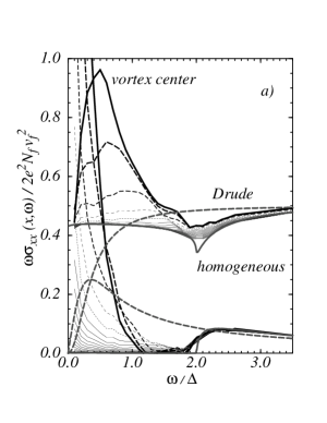
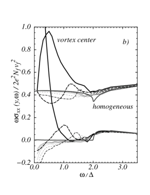
Figure 5: Frequency dependence of the real part (‘lower’ curves) and imaginary part (‘upper’ curves) of the local conductivity $\sigma_{xx}$ for a superconductor with parameters $T=0.3T_{c}$, $\ell=10\xi_{0}$. For convenience, the conductivities are multiplied by $\omega$. The full black curves give the conductivity at the vortex center, and the series of dashed lines with decreasing intensity the conductivity at increasing distance from the center. Fig.5a presents data at points along the $x$-axis (in steps of $(\pi/4)\xi_{0}$), and Fig.5b at points along the $y$-axis (in steps of $(\sqrt{3}\pi/4)\xi_{0}$). The dashed grey lines show the normal state Drude conductivity, and the full grey lines the conductivity of the homogeneous superconductor.

Figure 6: Local electrical field for a superconductor with parameters $T=0.3T_{c}$, $\ell=10\xi_{0}$, and an external frequency of $\omega=0.3\Delta(T)$. Each field pattern is a snapshot at time $t$ varying from 0 to half of time periode in timesteps of $\frac{1}{12}$ periode. The external electrical field $\delta\vec{E}^{\omega}(t)=\delta\vec{E}\cos(\omega t)$ is maximal and points in positive $x$-direction for the first picture ($t=0$). In the first picture of the second line it is zero. The distance between two points in the grid corresponds to $0.25\pi\xi_{0}$.

The frequency dependence of the local conductivity, $\sigma_{xx}(\vec{R},\omega)$, for $\vec{R}$ along the x- and y-axis is shown in figures 5a,b. These figures include, for comparison, the Drude conductivity of the normal state and the conductivity of the homogeneous bulk superconductor. A significant feature of conductivity in the core is the strong increase of ${\cal R}e\,\sigma$ at low frequencies. The conductivity is in this frequency range much larger than the normal state Drude conductivity and the exponentially small conductivity of the bulk s-wave superconductor. The real part of conductivity scales at low frequencies like $1/\omega^{2}$. Its value at at the vortex center is $69.5e^{2}N_{f}v_{f}^{2}/\Delta$ (outside the range of the figure) for $\omega=0.1\Delta$. The enhancement of the dissipative part at low frequencies is a consequence of the coupling of quasiparticles and collective order parameter modes, and cannot be obtained from non-selfconsistent calculations. Fig.5b shows that the real part of the conductivity becomes negative in the region of dipolar backflow on the $y$-axis. This leads locally to a negative time averaged power absorption, $<\vec{j}\cdot\vec{E}>_{t}\;<0$, and a corresponding gain in energy, which is compensated by the strongly enhanced dissipation of energy in the center of the vortex. The dissipative part of the local conductivity at a distance $R$ from the vortex center exhibits pronounced maxima whose frequencies increase with increasing $R$ and are given by 2$\times$ the energy at the maxima in the local density of states shown in Fig.2a. Hence, these features in the absorption spectrum must be identified as impurity assisted transitions between corresponding bound states at negative and positive energies. Impurities are required for breaking angular momentum conservation in these transitions.

The applied electric field $\delta\vec{E}(t)$ induces in the vortex core an internal field $-\vec{\nabla}\delta\varphi(t)$, which is of the same order as the applied field. Fig.6 shows the total electric field, $\delta\vec{E}_{tot}(t)=\delta\vec{E}^{\omega}(t)-\vec{\nabla}\delta\varphi(t)$, in the vortex core. The induced field is at low frequencies of dipolar form, and oscillates out of phase (phase shift $\pi/2$) with the applied field. This dipolar field originates from small charge fluctuation in the vortex core. At higher frequencies the dipolar field oscillates with a phase shift of $\approx\pi$, and screens part of the applied field.

We finally discuss the role of self-consistency in our calculation. Our results were obtained by iterating the self-consistency equations until the relative error stabilized below $\leq 10^{-10}$. Fig.7 compares the degree of violation of charge conservation in a non-selfconsistent calculation (no iteration) with the self-consistent result.

Figure 7: Degree of violation of charge conservation by the dissipative current flow for a non-selfconsistent calculation (Fig.7a), and a a self-consistent calculation (Fig.7b). The largest deviation in the non-selfconsistent calculation amounts to $\delta\dot{\rho}+\vec{\nabla}\delta\vec{j}=2.5e^{2}N_{f}v_{f}\delta E^{\omega}$. The data are obtained for a superconductor with $\ell=10\xi_{0}$ at $\omega=0.4\Delta(T)$ and $T=0.3T_{c}$.

We measure the degree of violation at position $\vec{R}$ by $D(\vec{R})=\max_{\,t}[\delta\dot{\rho}(\vec{R},t)+\vec{\nabla}\cdot\delta\vec{j}(\vec{R},t)]$. Charge conservation is obviously fulfilled if $D(\vec{R})=0$. The degree of violation at a point $\vec{R}$ is indicated in Fig.7a,b by the size of the filled circles around the grid points. The non-selfconsistent calculation (Fig.7a) results in a $D(\vec{R})$, which is much larger than the time derivative of the correct charge density, $\delta\dot{\rho}(\vec{R},t)$, obtained from a self-consistent calculation with $\delta\varphi(\vec{R},t)=0$ instead of charge neutrality condition. In Fig.7b we show the violation of charge conservation for our self-consistent calculation. The small remaining $D(\vec{R})$ is here a consequence of the finite grid size used in our calculations.

6 Discussion

This paper presented self-consistent calculations of the electromagnetic response of a pancake vortex in a superconductor with finite but long mean free path. This complements previous calculations for perfectly clean systems, which were done self-consistently in the limit $\omega\rightarrow 0$ ([Hsu93]), and at finite frequencies without a self-consistent determination of the order parameter ([Janko92], [Zhu93]).

The frequency range of interest in our calculations is of the order of the gap frequency, $\hbar\omega=\Delta$. We have shown that at low frequencies ($\hbar\omega<0.5\Delta$) the electromagnetic dissipation is strongly enhanced in the vortex cores above its normal state value, and that this effect is a consequence of the coupled dynamics of low-energy quasiparticles excitations bound to the vortex core and collective order parameter modes. The induced current density has at low frequencies a dipole-like behaviour, which results from an oscillating motion of the vortex perpendicular to direction of the driving a.c. field. The response of the vortex in the intermediate frequency range, $.5\Delta\la\hbar\omega\la 2\Delta$, is dominated by bound states in the vortex core. We find peaks in the local dissipation at twice the bound state energies. At higher frequencies, $\hbar\omega>2\Delta$, the conductivity approaches that of a very clean homogeneous superconductor, which is in good approximation given by the non-dissipative response of an ideal conductor.

References

• [1] Artemenko79Artemenko & Volkov 1979 Artemenko S.N., Volkov A.F. (1979): Usp. Fis. Nauk 128, 3, [Sov. Phys.-Usp. 22, 295].
• [2] Bardeen69Bardeen et al. 1969 Bardeen  J., Kümmel  R., Jacobs  A.E., Tewordt  L. (1969): Phys. Rev. 187, 556
• [3] Bardeen68Bardeen & Stephen 1965 Bardeen  J., Stephen  M.J. (1965): Phys. Rev. 140, A1197
• [4] Caroli64Caroli et al. 1964 Caroli  C., de Gennes  P.-G., Matricon  J. (1964): Phys. Lett 9, 307
• [5] Eschrig97Eschrig 1997 Eschrig  M. (1997): Ph.D. thesis, Bayreuth University (unpublished)
• [6] Hsu93Hsu 1993 Hsu  T.C. (1993): Physica C 213, 305
• [7] Janko92Jankó & Shore 1992 Jankó  Boldizsár, Shore  J.D. (1992): Phys. Rev. B 46, 9270-9273
• [8] Gorkov75Gorkov & Kopnin 1975 Gorkov  L.P., Kopnin  N.B. (1975): Usp. Fiz. Nauk 116, 413-448, [Sov. Phys.-Usp. 18, 496-513]
• [9] London50F. London 1950 London  F. (1950): Superfluids, Vol.1; Wiley, New York
• [10] Mattis58Mattis and Bardeen 1958 Mattis  D.C., Bardeen  J. (1958): Phys. Rev. 111, 412
• [11] nagat93Nagato et al. 1993 Nagato Y., Nagai K. and Hara J. (1993): J. Low Temp. Phys. 93, 33
• [12] Rainer96Rainer et al. 1996 Rainer  D., Sauls  J.A., Waxman  D. (1996), Phys. Rev. B 54, 10094
• [13] Rainer97Rainer & Sauls, this volume Rainer  D. and Sauls  J.A.: Introduction to Quasiclassical Theory, this volume
• [14] schop95Schopohl et al. 1995 Schopohl N. and Maki K. (1995): Phys. Rev. B 52, 490
• [15] Shelankov85Shelankov 1985 Shelankov  A.L. (1985): Journ. Low Temp. Phys. 60, 29-44
• [16] Zhu93Zhu et al. 1993 Zhu  Yu-Dong, Zhang  Fu-Chun, Drew  H.D. (1993): Phys. Rev. B 47, 586-588