.:plot:figure [
Magnetic correlations and quantum criticality in the insulating antiferromagnetic, insulating spin liquid, renormalized Fermi liquid, and metallic antiferromagnetic phases of the Mott system V2O3
Abstract
Magnetic correlations in all four phases of pure and doped vanadium sesquioxide () have been examined by magnetic thermal neutron scattering. Specifically, we have studied the antiferromagnetic and paramagnetic phases of metallic , the antiferromagnetic insulating and paramagnetic metallic phases of stoichiometric , and the antiferromagnetic and paramagnetic phases of insulating . While the antiferromagnetic insulator can be accounted for by a localized Heisenberg spin model, the long range order in the antiferromagnetic metal is an incommensurate spin-density-wave, resulting from a Fermi surface nesting instability. Spin dynamics in the strongly correlated metal are dominated by spin fluctuations with a “single lobe” spectrum in the Stoner electron-hole continuum. Furthermore, our results in metallic V2O3 represent an unprecedentedly complete characterization of the spin fluctuations near a metallic quantum critical point, and provide quantitative support for the self-consistent renormalization theory for itinerant antiferromagnets in the small moment limit. Dynamic magnetic correlations for in the paramagnetic insulator carry substantial magnetic spectral weight. However, they are extremely short-ranged, extending only to the nearest neighbors. The phase transition to the antiferromagnetic insulator, from the paramagnetic metal and the paramagnetic insulator, introduces a sudden switching of magnetic correlations to a different spatial periodicity which indicates a sudden change in the underlying spin Hamiltonian. To describe this phase transition and also the unusual short range order in the paramagnetic state, it seems necessary to take into account the orbital degrees of freedom associated with the degenerate -orbitals at the Fermi level in .
PACS number(s): 71.27.+a, 75.40.Gb, 75.30.Fv, 71.30.+h
]
I INTRODUCTION
The Mott metal-insulator transition[2] is a localization phenomenon driven by Coulomb repulsion between electrons. Mott insulators are common among transition metal oxides and are an important group of materials which cannot be accounted for by conventional band theories of solids. Using a simplified model which now bears his name,[3] Hubbard demonstrated a metal-insulator transition, in which a half-filled band is split by electronic correlations into upper (unfilled) and lower (filled) Hubbard bands.[4] His approach, however, failed to produce a Fermi surface on the metallic side of the Mott transition[5]. Also, there were unresolved questions concerning electronic spectral weight of the lower Hubbard band.[6] Starting from the metallic side, a Fermi liquid description of the correlated metal was provided by Brinkman and Rice[7]. They found that while the Pauli spin susceptibility, , and the Sommerfeld constant, , are both strongly enhanced by Coulomb repulsion, the Wilson ratio, , remains constant. Such behavior reflects a strongly enhanced effective mass and it was found that the metal to insulator transition could be associated with a divergence in the effective mass of these Fermionic quasi-particles.
The discovery of high temperature superconductivity in cuprates has revived interest in Mott systems[8]. To be precise, the cuprates are classified as charge transfer systems[9], but similar low energy physics is expected for both classes of materials. Progress in experimental techniques, such as photo-emission and X-ray absorption spectroscopy, has recently enabled direct measurements of the Hubbard bands and the Brinkman-Rice resonance.[10] On the theoretical side, there has also been progress especially in using infinite dimensional mean field theories[11] to calculate the local spectral function of the Hubbard model close to the metal-insulator transition[12]. A particularly important result is the synthesis of the seemingly contradictory pictures of Hubbard, Brinkman-Rice, and Slater on the metal-insulator transition in strongly correlated electron systems[13]. It is encouraging that these D= theories to a large extent reproduce the experimentally observed features[10] in the electronic density of states for three dimensional (3-D) transition metal oxides.
While there has been a remarkable convergence of experiments and theories which probe the electronic density of states across the Mott metal-insulator transition, little work has been done to explore magnetism close to this phase boundary for materials apart from the laminar cuprates. On the insulating side, the Heisenberg spin Hamiltonian was expected to offer a good description of magnetism but as we shall see in the following, this turns out not to be the case for systems with degenerate atomic orbitals. On the metallic side of the transition, one might have hoped that the local spin picture would survive because charge carriers in the Brinkman-Rice liquid are heavy and nearly localized. As we shall see this is also inconsistent with experiments. It turns out that the mobile quasi-particles have profound effects on magnetism in the metal. Indeed, the magnetism is that which one would associate with a quantum critical state, whose parameters are consistent with, for example, Moriya’s self-consistent renormalization (SCR) theory of metallic spin fluctuations[14, 15, 16, 17, 18, 19].
We obtained these surprising conclusions and others to be discussed below through a neutron scattering study of magnetic correlations in V2O3 and its doped derivatives which constitute a famous 3-D Mott system[20, 2]. Even though magnetic order occurs at low T in the metallic and the insulating phases of , the material is the only known transition metal oxide to display a Paramagnetic Metal (PM) to Paramagnetic Insulator (PI) transition (see Fig. 1). The PM
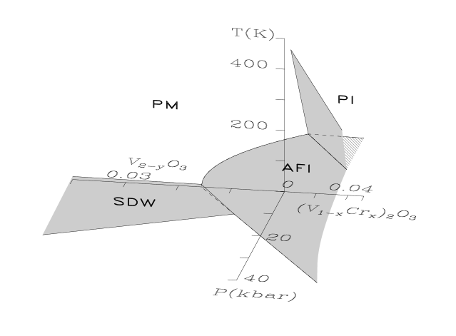
to Antiferromagnetic Insulator (AFI) transition in pure V2O3 is a spectacular first order phase transition in which the resistivity abruptly increases by 8 orders of magnitude[21, 22], the lattice structure changes from trigonal to monoclinic[23, 24], and the staggered moment immediately reaches over 80% of the low temperature ordered moment[25]. The mechanism for the phase transition remains controversial though it is clear that electron correlations are important because band structure calculations predict a metallic state for both the trigonal and monoclinic crystal structures.[26, 27] One explanation for the transition is due to Slater[28] who argued that the antiferromagnetic transition doubles the unit cell which in turn opens a gap at the Fermi energy. This mechanism however cannot account for the PM-PI transition and offers no explanation for the existence of the PI phase. Another viewpoint is that the AFI phase is simply the magnetically ordered state of the PI and that the Mott mechanism works for the PM-AFI transition as it does for the PM-PI transition. Following this approach, there have been various attempts to incorporate the antiferromagnetic phase in the framework of the Mott metal-insulator transition[29, 30, 31, 13]. However, none of the theories convincingly accounts for the first order nature of the PI-AFI transition observed in . Another shortcoming of the theories is that they assume that low energy and static magnetic correlations are characterized by the same wave vector throughout the phase diagram, something that our experiments show is not the case for the system.
Magnetic order and spin waves below 25 meV in the AFI phase of V2O3 were previously measured by other workers[25, 32, 33]. Our experiments are the first neutron scattering study of magnetic correlations in the AFM, PM and PI phases of V2O3. Our most important conclusions are the following: (1) the AFM has a small moment incommensurate spin-density-wave (SDW) at low temperatures, which results from a Fermi surface instability. (2) Dynamic spin correlations in the entire PM phase are controlled by the same Fermi surface instability. (3) Magnetic correlations in the metallic phases are those one might expect near a quantum critical point. They are quantitatively described by the SCR theory for itinerant antiferromagnetism in the small moment limit. (4) Anomalously short-range dynamic spin correlations in the PI are closely related to those in the PM but are different from the magnetic order in the AFI. (5) Phase transitions to the AFI, from either the PM or the PI, cause an abrupt switch of the magnetic wave vector, signaling a sudden change of the exchange constants in the spin Hamiltonian. All of (1)-(5) require more than a conventional Heisenberg spin Hamiltonian for a satisfactory explanation. In metallic samples the geometry of the Fermi surface directly affects magnetic correlations, while in insulating samples there are low energy orbital degrees of freedom which are important for describing the unusual PI phase and the PI-AFI phase transition. Some of the above results were previously published in short reports[34, 35, 36, 37, 38, 39, 40].
The organization of the paper is as follows. Section II covers experimental details concerning sample preparation and neutron scattering instrumentation, sections III, IV, V and VI describe magnetic correlations in the AFM, PM, AFI and PI phases respectively, and section VII concludes the paper with a discussion of the overall interpretation of the data.
II EXPERIMENTAL DETAILS
in all but the AFI phase, where small lattice distortions break the three fold rotation symmetry to yield a monoclinic structure.[24] We use the conventional hexagonal unit cell[34, 21] with six V2O3 formula units per unit cell to index real and reciprocal space. The reciprocal lattice parameters are and in the metallic phases, and in the AFI phase, and and in the PI phase. More accurate values of lattice parameters, as functions of temperature and doping, can be found in Ref. [[23, 42, 43]]. With this unit cell, the characteristic wave-vector of the AFI spin structure[25] is (1/2,1/2,0) while it is (0,0,1.7) for the SDW structure[34] (refer to Fig. 3).
Samples were oriented in either the () or the () zone to reach peaks in the neutron scattering associated with the two types of magnetic correlations. Selection rules for nuclear Bragg points in these two zones are (): and (): , .
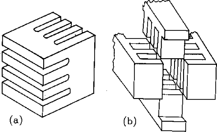
Single crystals of V2-yO3 were grown using a skull melter[44]. The stoichiometry of pure V2O3 and metal-deficient V2-yO3 was controlled to within by annealing sliced, as-grown V2O3 crystals in a suitably chosen CO-CO2 atmosphere[45] for two weeks at 1400oC. Single crystals of (V1-xCrx)2O3 were grown using the Tri-arc technique[22]. The compositions were determined by atomic absorption spectroscopy and wet chemical titration technique. The mass of samples for elastic neutron scattering was typically 100 mg, while we used several grams for inelastic neutron scattering experiments. Large single crystals were sliced into plates of 1.5 mm thickness as shown in Fig. 4(a) to allow oxygen
diffusion to the bulk during the annealing process. Several single crystals of each composition were mutually aligned to increase the sensitivity for inelastic measurements. We report experiments for the seven compositions which are listed in Table I. The samples
| 0 K | 300 K | |||
|---|---|---|---|---|
| V1.963O3 | SDW | PM | ||
| V1.973O3 | SDW | PM | ||
| V1.983O3 | SDW | PM | ||
| V1.985O3 | AFI | PM | ||
| V1.988O3 | AFI | PM | ||
| V2O3 | AFI | PM | ||
| V1.944Cr0.056O3 | AFI | PI |
have been well characterized in previous studies using bulk measurement techniques[22, 46, 47, 48, 49, 50].
The sample temperature was controlled using liquid He flow cryostats in the range from 1.4 K to 293 K, or using displex closed cycle cryostats from 10 K to 293 K. With a heating element, the displex cryostat could reach temperatures up to 600 K.
Hydrostatic pressure up to 8 kbar was produced using a He gas high pressure apparatus[51] at NIST, which can be loaded into an “orange” ILL cryostat with a temperature range from 1.4 K to room temperature.
A Neutron Scattering Instrumentation
Neutron scattering measurements were performed on triple-axis spectrometers BT2, BT4 and BT9 at the NIST research reactor, on HB1 at the High Flux Isotope Reactor (HFIR) of ORNL, and on H4M and H7 at the High Flux Beam Reactor (HFBR) of BNL. For unpolarized neutron experiments, we used a Be (101) monochromator on HB1, Cu (220) and pyrolytic graphite (PG) (002) monochromators on BT4 and PG (002) monochromators on all other instruments. PG (002) analyzers were used for all unpolarized triple-axis experiments. For polarized neutron measurements on BT2, crystals of Heusler alloy Cu2MnAl [(111)=3.445] were used as monochromator and analyzer. Fast neutrons were removed from the incident beam by an in-pile sapphire filter[52] on HB1, and PG filters[53] were used to remove high-order neutron contaminations where appropriate. The horizontal collimations were controlled with Soller slits and are specified in the figures containing the experimental data. The fast neutron background at BT4 in the small scattering angle limit was reduced by a 30 cm long boron-polyethylene aperture before the sample and a similar 15 cm long aperture after the sample. The opening of the aperture was adjusted to match the sample size (Fig. 4(b)). These apertures suppress fast neutron background in the small angle limit which is important for measuring high energy inelastic magnetic scattering.
In most of our scans, the background is approximately constant. For some scans, however, the scattering angle falls below where background increases rapidly with decreasing angle. For example, a constant-meV scan measured with H4M is shown in Fig. 5 with solid circles.

The scattering angle at (100) is 5.4o. As a result, the background (open symbols), measured with the analyzer turned 10o from the reflection condition, increases near (100). The solid line represents data with this extra background contribution subtracted[54].
B Neutron Scattering Cross Section
The magnetic neutron scattering cross-section for momentum transfer and energy transfer is given by [55]
| (1) | |||||
| (2) |
where is the number of hexagonal unit cells, barn/, is the magnetic form factor for the V3+ ion[56], is the Debye-Waller factor, and the dynamical structure factor is given by
| (4) | |||||
is the Landé factor, is the th Cartesian spin component of the V ion at position R at time , and denotes a thermal average. When spin space anisotropy can be neglected, as in the paramagnetic phase of a Heisenberg system, expression (2) simplifies to
| (5) |
We will drop the superscripts in the remaining text for brevity. The structure factor is related to the imaginary part of the dynamic spin susceptibility by the fluctuation-dissipation theorem
| (6) |
The real part of the generalized spin susceptibility is given by the Kramers-Kronig relation,
| (7) |
The intensity in a neutron scattering experiment is measured as the ratio of neutron counts in a high efficiency 3He detector to the neutron counts in a low efficiency monitor placed in the incident beam before the sample. To cover a wide energy range of spin excitations, several spectrometer configurations were used. The relative sensitivity of different configurations was determined by comparing the integrated intensities of identical scans probing magnetic or incoherent nuclear scattering. Normalizing to inelastic scattering from acoustic phonons[57, 58] yielded absolute measurements of [Eq. (4)] in units of /meV. Units of mbarn/meV are also used in this paper and when we do so we are quoting numbers for the following normalized intensity
| (8) |
which is more directly related to the raw data because it contains the magnetic form factor, , as a factor.
C Resolution Effects
The measured intensity in a neutron scattering experiment is proportional to the convolution of the scattering cross-section with an instrumental resolution function. The resolution function can be approximated by a Gaussian function in 4-dimensional q- space[59, 60]. Inelastic neutron scattering experiments are usually flux-limited. Therefore the choice of an experimental configuration for probing a specific scattering cross section always involves a trade-off between resolution and sensitivity. The following two limits are of importance in this study.
1 Infinite life time excitations
Examples of this type of excitations, such as phonons and un-damped antiferromagnetic spin waves, are described by a scattering cross section of the form
If the curvature of the dispersion surface is negligible over the volume of the resolution function then the dispersion surface can be approximated by a flat plane and the resulting profile of a scan through the dispersion surface is approximately Gaussian with a width defined by the resolution. With coarser resolution, the profile becomes asymmetric and the peak position may shift from the position defined by the dispersion relation. Refer to the dotted lines in Fig. 10 for a few examples of such effects.
2 Weakly and dependent scattering cross section
Features in the scattering cross-section which are broader in - space than the experimental resolution are reproduced directly or with slight additional broadening in the measured and dependent intensity. This is the case for our measurements in the AFM, PM and PI phases. For example if takes the form
a constant energy scan will yield a Gaussian peak with width , where is the resolution width. To appreciate the resolution broadening, let us put in numbers: When the resolution width is 1/3 of the intrinsic width, the measured width increases by less than 10% over the intrinsic width. When the resolution width is 1/5 of the intrinsic width, the measured width is only 2% larger than the intrinsic width. In this latter case the measured intensity is then very close to being directly proportional to .
III SDW in metallic V2O3
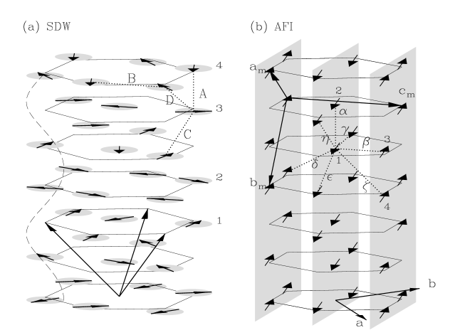
The insulating antiferromagnetic state (AFI) of V2O3 can be suppressed by a pressure of 20 kbar[61, 50]. The pressure-stabilized metallic state is paramagnetic down to at least 0.35 K.[62, 50] The AFI state can also be suppressed at ambient pressure by vanadium deficiency[63] or titanium doping[20]. The critical concentrations are for V2-xTixO3[20] and for V2-yO3[46]. The existence of antiferromagnetic order at low temperatures for the doping induced metal was first established through the 57Fe Mössbauer effect[64, 65, 66]. The magnetic structure was only recently determined through single crystal neutron diffraction[34], and it is depicted in Fig. 3 (a). This magnetic order can be described as puckered antiferromagnetic honeycomb spin layers whose spin directions form a helix along the axis. The spin directions determined from our neutron diffraction refinement, which lie in the basal plane, are consistent with previous susceptibility anisotropy and magneto-torque measurements[65, 67]. The pitch of the helix yields an incommensurate magnetic structure, with magnetic wave vector 1.7c∗. Both the staggered moment and the wave vector depend weakly on doping, .[34] This magnetic order in metallic bears little resemblance to the magnetic order in the insulating phase of which is characterized by a magnetic wave vector (1/2,1/2,0)[25] [refer to Fig. 3 (b)].
We have previously shown[34] that the antiferromagnetic order in the metallic state can not be described by a localized spin model, since the dynamic magnetic spectral weight greatly exceeds the square of the staggered moment and the bandwidth for magnetic excitations exceeds kBTN by more than one order of magnitude. The proper concept is probably that of a spin density wave[68, 69, 70] where magnetic order results from a Fermi surface nesting instability. This interpretation is supported by recent RPA calculation of the q-dependent susceptibility using realistic band structure[71]. According to neutron, specific heat, and transport measurements, only a small fraction of a large Fermi surface[34] is involved in the SDW of metallic V2-yO3. As seen at the SDW transition for Cr metal[72], the resistivity for metallic V2-yO3 increases below the Néel temperature as the Fermi surface is partially gapped.[34] This is in contrast to localized spin systems where the resistivity decreases below because of the decrease in spin disorder scattering. The discovery of the transverse incommensurate SDW resolved the longstanding mystery[73] about the magnetic ground state of doped metallic V2O3.
A Polarized neutron scattering
To further characterize the incommensurate magnetic structure, polarized neutron measurements were performed. A V1.983O3 sample was oriented with its (0) zone in the horizontal scattering plane. A small magnetic field of 7.6 G was applied along either the scattering wave vector (HF) or along the vertical direction (VF) to guide the neutron spin. A neutron spin flipper was inserted in the neutron path. In the HF case when the spin flipper is turned on, only magnetic scattering contributes to the Bragg peak[74]. Coherent nuclear scattering is non-spin-flip and contributes when the flipper is off. Therefore, Fig. 6(a) shows that the (1,0,)
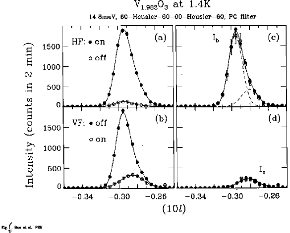
Bragg peak is indeed magnetic. The finite intensity in the flipper off case is due to incomplete polarization of the neutron beam and is consistent with a flipping ratio of =14, measured at nuclear Bragg peaks.
Since , (1,0,) is essentially parallel to the a∗ axis. The four partial intensities at (1,0,) for the HF and VF cases with the spin flipper on or off are therefore[74]
| (10) | |||||
| (11) | |||||
| (12) | |||||
| (13) |
where is the contribution from the spin components in the (or c) direction, and is the flipping ratio in the HF (VF) case. Therefore, from the data shown in Fig. 6 (a) and (b), and can be extracted by solving the over-determined equations (10)-(13). For example,
| (15) | |||||
| (16) | |||||
| (17) | |||||
| (18) |
In the last step in (III A), a small quantity is neglected. Alternatively,
| (20) | |||||
| (21) | |||||
| (22) | |||||
| (23) |
Fig. 6 (c) and (d) show the basal plane component and the vertical component derived from the data in Fig. 6 (a) and (b) using these expressions. The solid circles were determined using Eq. (III A) and the open circles using Eq. (III A). The two data sets are consistent within experimental uncertainty and show that the incommensurate peak is associated with basal plane spin correlations as was previously conjectured on the basis of unpolarized neutron diffraction. The data also reveal a second incommensurate peak with mixed polarization. This peak has only been observed in this sample which is very close to the critical concentration, , for the ambient pressure metallic phase [34].
When polarized neutrons are scattered by a right-handed transverse spiral in the HF configuration, the partial cross-sections for magnetic Bragg peaks with wave vectors along the spiral axis are[74]
| (24) | |||||
| (25) |
for the neutron spin up to spin down channel and
| (26) | |||||
| (27) |
for the neutron spin down to spin up channel. In these expressions the nuclear reciprocal lattice vector and the spiral wave vector, , are both parallel to the spiral axis. Note that only one of the two magnetic satellite Bragg peaks appears in each channel. For a left-handed spiral, the signs of in these expressions reverse. Therefore if the SDW in is a spiral with a macroscopic handedness, we should find that magnetic Bragg peaks with come and go with a 180o rotation of the incident neutron spin state.
Fig. 7 shows a double-axis polarized neutron scan through
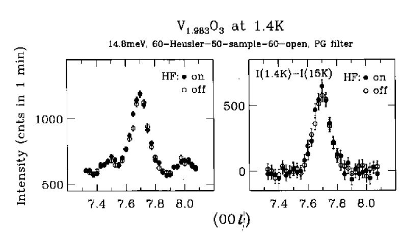
the (0,0,7.7) magnetic Bragg peak of the SDW. The left panel shows raw data taken at 1.4 K, while in the right panel, a non-magnetic background taken above the Néel temperature has been subtracted. Clearly the magnetic Bragg intensity does not change upon flipping the incident neutron spin state. Hence we conclude that the SDW phase does not have an intrinsic macroscopic handedness. This means that if the ordered phase is a spiral, our sample contains equal volume fractions of left and right handed spirals. Another possibility is that we have an amplitude modulated SDW which is a microscopic superposition of the left and right-handed spirals.
B SDW, PM and AFI phase boundary at T=0
After confirming the magnetic structure in the AFM phase with polarized neutrons, let us now try to delimit the phase boundary of this SDW ground state in the pressure-composition plane for V2-yO3. Two of the samples we studied with high pressure neutron diffraction ( and 0.015) have the AFI ground state at ambient pressure and display the metallic state only under pressure. Fig. 8 (a) shows the (1/2,1/2,0) Bragg peak which is the order parameter
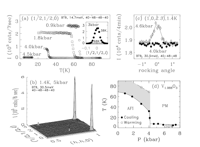
of the AFI, as a function of temperature at various pressures for a V1.988O3 sample. Under high pressure, the transition to the AFI remains strongly first-order, as shown here by the sudden onset of antiferromagnetic order with a nearly saturated magnetic moment.
The AFI state is completely suppressed above 4.1 kbar for V1.988O3. A survey at 5 kbar and 1.4 K in a quadrant of the () Brillouin zone reveals no magnetic peaks associated with the AFI phase [refer to Fig. 8 (b)]. On the other hand the Bragg peaks associated with SDW order are absent for P=4.0 kbar but appear under a pressure of 4.6 kbar [refer to Fig. 8 (c)]. The temperature-pressure phase diagram for V1.988O3 is shown in Fig. 8 (d). The SDW transition is second order,[34, 37] while the first order AFI transition shows large thermal hysteresis.
Fig. 9 summarizes our current knowledge about ground
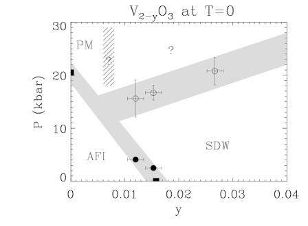
states in V2-yO3. For , after the AFI is suppressed, the metallic state is paramagnetic. For and 0.015, we found that after the AFI is suppressed, the metallic state is a SDW. Up to 8 kbar, the upper limit of our pressure cell, the SDW remains the stable low temperature state for all the samples (, 0.015 and 0.027) which we have studied with high pressure neutron diffraction[34, 37]. By linear extrapolation of the pressure dependent Néel temperatures, we derived estimates for the critical pressures of the SDW phase and these are indicated by open circles in Fig. 9.
Anderson has pointed out the possibility of a superconducting instability in the Brinkman-Rice liquid[75]. For metallic V2-yO3, SDW order appears to be the dominant instability. However, it should be noted that the possibility of a superconducting state with K at high pressures has not been excluded yet[76].
IV Spin excitations and quantum critical behavior in metallic phases
A Stoner electron-hole pair continuum at
Fig. 10 shows constant energy transfer, ,

scans spanning a whole Brillouin zone in the AFM phase for V1.973O3 (T K). The incommensurate Bragg points, (1,0,) and (1,0,2.3), covered by these scans correspond to the long range ordered SDW. The solid circles represent a flat background measured by turning the PG(002) analyzer 10o away from the reflection condition. Around each magnetic Bragg point, (1,0,) or (1,0,2.3), there is only one broad peak. This is not due to poor resolution merging two counter-propagating spin wave modes: the dotted lines in the figure represent the calculated spectrometer response to spin waves with a velocity meV, which is much larger than the inverse slope of the peak width versus energy transfer curve (see Fig. 11). Our resolution is clearly adequate to rule

out a conventional spin wave response in this energy range. Therefore the broad intensity profile which we observed is intrinsic, and in the energy range probed, magnetic excitations consist of a single broad lobe at each magnetic Bragg point.
For insulating magnets, propagating spin waves exist over the whole Brillouin zone. For itinerant magnets, however, propagating spin waves only exist in a limited range near the magnetic Bragg peaks. Beyond this range they merge into the Stoner particle-hole continuum. According to weak coupling theory,[70] the energy gap which a SDW creates inside the particle-hole continuum is , where and and are Fermi velocities of the two nesting bands. Inside this gap, spin waves propagate with a velocity[70, 77, 78] . For metallic V2-yO3 at T=0, spin waves are expected only below meV, which is below the energies which we have probed in this experiment. The broad lobes measured in Fig. 10 thus represent magnetic excitations inside the Stoner continuum.
Other signs that we are probing magnetic fluctuations in the electron-hole continuum, as opposed to transverse oscillations of the order parameter, are (1) The spectral weight from 1.5 meV to 18 meV in Fig. 10 corresponds to a fluctuating moment of 0.32 per V, already twice that of the static staggered moment,[34] and (2) The resolution corrected full-widths-at-half-maximum (FWHM) of constant energy scans (see Fig. 11) extrapolate to a finite value at , even though there are true, resolution-limited, Bragg peaks at .
For Cr metal[79, 80], another 3-D SDW (T K), one would expect at T=0 that spin wave modes merge into a single broad lobe above 1.76=47 meV. However, due to the much larger spin wave velocity in Cr, estimated at 1000 meV[81, 82], it has not yet been possible in this material to distinguish between resolution merged spin waves and single lobe excitations. We were aided in the case of metallic V2O3 by strong correlations. The enhanced effective mass reduces the Fermi velocity to a value which is of that for Cr.[34] This makes it feasible to unambiguously observe these unique single-lobe magnetic excitations in the SDW state of V2-yO3.
B Doping effects in the metallic phases
We have previously shown[34] that both the staggered moment and the incommensurate wave vector of the static SDW order depend only weakly on doping. For a change in metal-deficiency which is twice the critical for the AFI phase, the change in the magnetic wave vector (1.7c∗) is only 0.02c∗. Likewise, dynamic magnetic correlations in the PM phase are insensitive to doping. As shown in Fig. 12,

even for pure V2O3 which has different low temperature AFI state, the magnetic response at 200 K is indistinguishable from that of V1.973O3. In particular we do observe peaks at the SDW wave vectors. This demonstrates that magnetism throughout the metallic phase is controlled by the same Fermi surface instability and indicates that small moment incommensurate antiferromagnetism in is not due to impurity effects but is an intrinsic property of metallic .
C Antiferromagnetic quantum critical behavior in metal
The SDW in metallic V2-yO3 is a small moment, low temperature antiferromagnetic ordering. The staggered moment in the magnetic ground state (0.15) is only a small fraction of the effective paramagnetic moment (2.37-2.69) which appears in the high temperature Curie-Weiss susceptibility[83, 84, 67]. In other words, the magnetic system is very close to a quantum critical point[85, 86, 87, 88]. We have previously shown[37] that the single lobe spin excitation spectrum in metallic V1.973O3 is isotropic in space, and the spectrum , from 1.4K inside the ordered phase to temperatures above 20TN, has been determined in absolute units[89]. Here we discuss our results in connection with the quantum critical behavior.
Fig. 13(a) shows in a log-log scale

the inverse correlation length, , measured in Ref. [[37]] as a function of the reduced temperature, . The solid line is with from a least squares fit. This value of suggests a small positive exponent according to the scaling relation[90] . However, the classical values of are also consistent with our data (refer to the dotted line).
The spin fluctuation spectrum reaches its maximum value, , at and which is an antiferromagnetic Bragg point[37]. The dominant part of the spectral weight, therefore, falls in the hydrodynamic region[91], , where . In Fig. 13(b), we find the dynamic exponent (the solid line), which is in agreement with the theoretical prediction for itinerant antiferromagnets in the quantum critical region[85, 88]. The constant prefactor is meV.
Combining the scaling relations from Fig. 13(a) and (b), we have [refer to the solid line in Fig. 13(c)]. Given the small value of and the fact that , the characteristic spin fluctuation energy is close to [refer to the dotted line in Fig. 13(c)]. This feature is shared with nearly metallic cuprates[92] and some heavy fermion systems[93]. Antiferromagnetic spin fluctuations for systems close to a quantum critical point, therefore, might provide a microscopic mechanism for marginal Fermi liquid phenomenology[94].
The peak intensity of some constant energy scans is shown in Fig. 14(a) as function of energy.

They are expressed in absolute units and represent at the magnetic zone center. At 1.5K, is a decreasing function of in the measured energy range and it changes to an increasing function at elevated temperatures. They were scaled onto a single universal curve in Fig. 14(b) by dividing by and by the peak energy . The apparently different behaviors in a finite energy window in Fig. 14(a), therefore, reflect different segments of a universal behavior.
For a general wave vector, , away from an antiferromagnetic Bragg point, , we have shown[37] previously that our neutron scattering data measured at various temperatures can be described by
| (28) |
where the scaling function is
| (29) |
The solid line in Fig. 14(b) is . The maximum is related to static staggered susceptibility[37]. Combining Kramers-Kronig relation and Eq. (28) gives
| (30) | |||||
| (31) | |||||
| (32) | |||||
| (33) |
Notice that when , , and , hence Eq. (28) becomes
| (34) |
where and are non-universal constants.[95] Using from our measurement and the scaling relation , and absorbing the constant in the scaling function,
| (35) |
This expression, which is supported by our experimental data, is identical to the scaling form proposed by Sachdev and Ye in the quantum critical region[87].
D Theory of itinerant magnetism
Itinerant magnetic systems have been studied within the random-phase approximation (RPA), which provides a reasonable description at T=0 for the ordered moment and for spin excitations in the spin wave modes and in the Stoner continuum. But it does not relate the low-temperature excitation parameters to finite-temperature properties such as the ordering temperature and the high temperature Curie-Weiss susceptibility.
The imaginary part of the RPA generalized susceptibility for an itinerant antiferromagnet, as was done to describe magnetic fluctuations in chromium[77, 78], can be written as follows:
| (36) |
where the wave vector dependent relaxation rate,
| (37) |
corresponds to the simplest functional form consistent with the dynamical scaling hypothesis with a dynamic exponent . As a comparison, for the insulating Heisenberg antiferromagnet,[91, 98] . The uniform non-interacting susceptibility , the length scale , and are temperature-independent parameters, and the inverse correlation length approaches zero when the Néel temperature is approached. This functional form and derivations thereupon[99] offer a good description of critical spin fluctuations for Cr and its alloys[82, 100]. They have also been successfully used to describe spin dynamics as measured by neutron scattering for La1.86Sr0.14CuO2 above the superconducting transition temperature[101]. A modified form was used to model nuclear magnetic resonance (NMR) data in other high temperature superconducting cuprates[102, 103, 104]. However, the RPA parameters , , and in Eq. (36) are free parameters which are not connected to other physically measurable quantities.
The SCR theory,[15, 16, 17, 18, 19] a mode-mode coupling theory, improves upon the RPA theory by considering self-consistently the effects of spin fluctuations on the thermal equilibrium state. It is solvable in the small moment limit with a few experimentally measurable parameters. The ferromagnetic version of the SCR theory was discussed in [[15, 16, 17, 18]] and the antiferromagnetic version in [[19, 96]].
The generalized susceptibility for antiferromagnets in the SCR theory[96] has the same functional form as in the RPA theory:
| (38) |
where is defined as in Eq. (37). The RPA parameter is substituted now by the static staggered susceptibility , in consistence with the Kramers-Kronig relation. Major difference from the RPA theory, however, is that the SCR theory can predict other physical quantities using parameters from spin excitation spectrum[97]. For example, the non-universal parameters[95] and defined above Eq. (34) can be used to quantitatively relate to the staggered moment (refer to Fig. 4 of Ref. [[37]]).
Fig. 15 shows an example of a simultaneous fit of

constant energy scans to Eq. (38) and (37) for stoichiometric V2O3 at 200K. Solid circles represent the magnetic response in the paramagnetic metallic phase, which peaks around the SDW wave vectors. The resolution widths are much smaller than the measured widths, therefore resolution broadening can be ignored in this case. The solid line through these 200K data is the best-fit functional form for calculated using copies of Eq. (38) summed over the Bragg points and with , , meV/ and /meV per vanadium. These values are within the error-bars of those for V1.973O3,[37] as should be expected given the close similarity of the raw data for these two samples which are shown in Fig. 12.
It is customary to use the Lorentzian relaxation energy of (36) or (38) as the energy scale of spin fluctuations. For an itinerant antiferromagnet close to a quantum critical point, such as metallic V2-yO3, this reduces to at [37]. To demonstrate the prominence of this energy, we plot in Fig. 16(a)
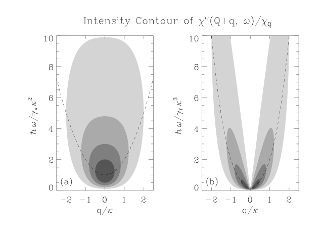
the intensity contour of for small moment itinerant antiferromagnets [refer to Eq. (38), (37) and (29)]. The spectrum is unique in that the electron-hole damping has reduced the excitation spectrum to a single lobe at the magnetic zone center, as we observed in our neutron scattering experiment for metallic V2-yO3[34, 38]. The peak intensity occurs at and , and clearly is the characteristic energy scale. In this case, , as we found experimentally, is essential for achieving the quantum critical scaling of (35).
This is quite different from the well studied case of small moment itinerant ferromagnets. The predicted by the SCR theory for ferromagnets[105, 106] has the same Lorentzian form as (38), but the relaxation energy is given by
| (39) |
Like the antiferromagnetic SCR theory, the ferromagnetic SCR theory not only correctly describes the spin fluctuation spectrum, but also quantitatively relates the spectrum parameters to various other physical quantities, as demonstrated in the 3-D small-moment ferromagnets MnSi[58, 106, 107] and Ni3Al[105]. Recasting Eq. (38) and (39) in a dimensionless form,
| (40) |
with
| (41) |
It is depicted in Fig. 16(b). Although the counter-propagating spin wave branches are over-damped by electron-hole excitations, they remain two separate branches. The intensity is singular at and , and the Lorentzian relaxation energy (the dashed line) serves well as the energy scale in this case, as customarily performed.
V Spin waves in the AFI phase
While magnetic excitations in the metallic phase are dominated by over-damped modes, the AFI phase exhibits conventional propagating spin wave excitations. Word et al. [32] measured spin waves in this phase around (1/2,1/2,0) at 142K in pure V2O3. There is a spin excitation gap of 4.8 meV, which is essentially independent of temperature for [33]. For V1.94Cr0.06O3 (TN=177K), the gap energy at (1/2,1/2,0) is not different from that seen for the pure sample for temperatures below 50K[33]. However, it shows substantial softening with rising temperature, consistent with the trend towards a continuous phase transition with increasing Cr doping.
Here we present spin waves measured at 11 K for V1.944Cr0.056O3. Fig. 17 shows constant energy scans

near a magnetic zone center. The spin wave dispersion relation has been measured for energies up to 50 meV (see Fig. 18)

which covers about one quarter of the Brillouin zone. For comparison, some of previous data for pure V2O3 are also included in Fig. 18. At low measurement temperatures and for meV, there is no difference in the spin wave dispersion for pure and 3% Cr doped V2O3.
Spin waves in the isomorphous corundum antiferromagnets Cr2O3 and -Fe2O3 have been measured over the whole Brillouin zone[108, 109]. These two compounds have different magnetic structures[110, 111]. Linear spin wave theory[112] using the Heisenberg Hamiltonian
| (42) |
satisfactorily describe the experimental dispersion relation. The dominant exchange constants for Cr2O3 are and meV between spin pairs and respectively[108] (refer to Fig. 3), while for -Fe2O3 spin pairs and interact most strongly with exchange constants and meV respectively.[109] In V2O3, the corundum symmetry is broken[113, 24] at the AFI transition. Consequently there are seven different exchange constants between these spin pairs [refer to Fig.3(b)].
Dispersion relations for spin waves in the AFI phase of are derived in Appendix A following the procedure described by Sáenz[114]. The limited data in Fig. 18 do not allow reliable determination of individual exchange constants. Along the direction the acoustic spin wave has a simple dispersion relation
| (44) | |||||
In combination with the previously measured value of the ordered moment ([25]) our measurements of this dispersion relation permits the local anisotropy field, meV, and meV to be determined with confidence.[115] To determine the individual exchange constants, experiments which will measure spin waves in the AFI across the whole Brillouin zone are now under way.
VI The insulating spin liquid
The solid circles in Fig. 19 represent constant energy scans
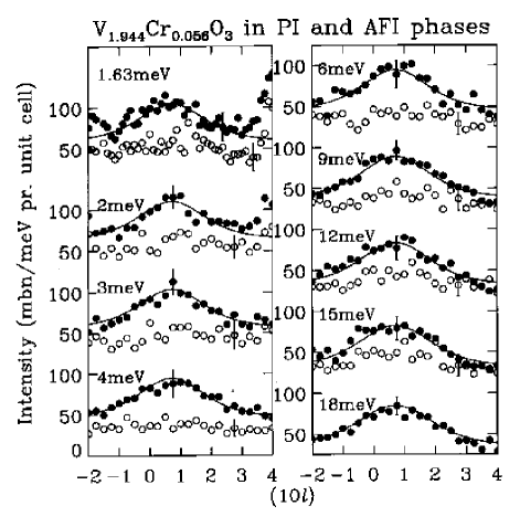
along (10) at 205K in the PI phase of V1.944Cr0.056O3. The peak profile is not sensitive to energy transfer for 1.6 meV18 meV. The peaks are very broad and the half-width-at-half-maximum (HWHM) corresponds to a correlation length in the c direction. Scans in the basal plane (refer to Fig. 20)

also yielded broad -insensitive peaks, corresponding to in the a direction. These correlation lengths extend only to the nearest neighbors in the respective directions and they are even shorter than in the PM phase at comparable temperatures, as can be ascertained by comparing Fig. 12 or Fig. 15 to Fig. 19. This is a surprising result because the electron-hole pair damping mechanism which exists in the metal is inhibited by the charge excitation gap of the insulator.
The effect of temperature on the short-range magnetic correlations in the PI phase is shown in Fig. 21. Data for two
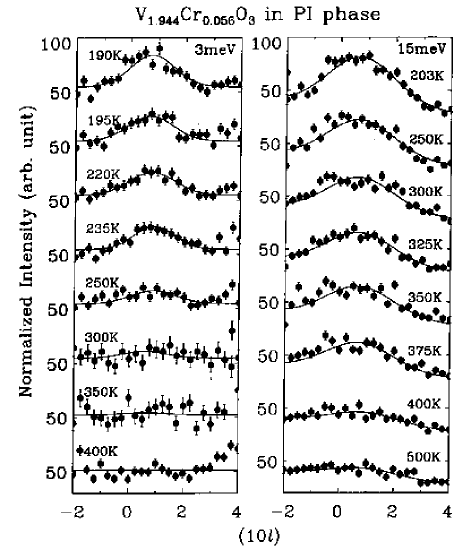
values of energy transfer are shown. Clearly, q-dependent magnetic scattering is suppressed at high temperatures. Even so, there is no discernible narrowing of the peak, even as the AFI transition temperature, K, is approached. Thus, does not appear to be the critical temperature for spin fluctuations in the PI. As for stoichiometric V2O3 (refer to Fig. 15), the characteristic wave vector for magnetic correlations of Cr-doped V2O3 moves to another part of reciprocal space in the AFI phase[38] leaving a flat background as shown by open circles in Fig. 19. Therefore, the phase transition to the AFI is not a conventional antiferromagnetic transition, for which the correlation length diverges at and magnetic Bragg peaks emerge from peaks in the paramagnetic response function. Instead, the spin Hamiltonian is altered by some underlying processes.
Not only is the location in reciprocal space of the paramagnetic neutron scattering in the PI phase unusual, but also is the and dependence of scattering about this location. For conventional insulating antiferromagnets, when the correlation length is limited to the nearest neighbor spin spacing by thermal fluctuations at , there is very little spectral weight in the modulated part of the dynamic correlation function. In the PI phase of , however, constant energy cuts through show that large spectral weight ( per V, see below) is associated with a ridge along which forms a very broad peak in -space. These experimental results suggest that the spin-spin interaction strength is not dwarfed by the thermal energy and that a mechanism other than thermal fluctuations therefore must be responsible for limiting magnetic correlations to nearest neighbors.
One possible mechanism is geometric frustration where conflicting magnetic interactions prevent long range order at . Solid state chemistry, however, does not support this explanation because the dominant exchange interactions in Heisenberg models for corundum antiferromagnets in general are not frustrated[116, 117]. Disorder introduced by Cr doping is also unlikely to be important, since for the same sample at low temperatures, spin waves in the AFI phase are resolution-limited (refer to section V and Fig. 3 in Ref. [38]). A very promising explanation, based on the electronic state of V2O3 in the single ion limit, was recently proposed by Rice[118, 38]. Each magnetically active electron on a vanadium ion can exist in one of the two doubly degenerate orbitals.[41] The orbital degeneracy may be the source of large orbital contribution to the nuclear relaxation[119]. Depending on the relative occupation of these two degenerate orbitals on neighboring sites, the exchange interaction between spins on these sites can have different signs[120]. In the PI phase, the orbital occupation is fluctuating and disordered, resulting in a spin Hamiltonian with fluctuating exchange interactions of different signs which induce local antiferromagnetic correlations, while dephase longer range correlations. We will return to this idea in section VII.
A Analysis of spatial correlations
A consequence of the -insensitive peak width in the PI phase (Fig. 19 and 20) is that constant energy scans directly probe the -dependence of the instantaneous spin correlation function. Because of the short correlation lengths, the spatial dependence of the magnetic correlations can be modeled by a finite spin cluster which includes the four types of near neighbor spin pairs: , , and [refer to Fig. 3(a)]. In other words, the summation in the structure factor
| (45) |
needs only include one -type spin pair, three -type spin pairs, three -type spin pairs and six -type spin pairs for any one spin, , of the spins in a hexagonal unit cell.
In Fig. 22, an extended scan along the c axis,

covering more than three Brillouin zones, and scans in the basal plane intersecting the peaks near the (101) and (10) are shown for V1.944Cr0.056O3 at 205 K in the PI phase. Background measured at 160K in the AFI phase is also shown. A good approximation to the magnetic intensity at 205 K is obtained by subtracting the 160 K background and such difference data are shown in Fig. 23.

The dotted line indicates the magnetic form factor for the ion[56], . Extra intensity at large is attributed to incomplete subtraction of phonon neutron scattering. A simultaneous fit of to the magnetic intensity from these 3 meV scans is shown as solid lines in Fig. 23. As can be seen in the figure this spin cluster model is consistent with the data over the large part of q-space where the magnetic form factor is appreciable.
The near-neighbor spin correlations derived from the best fit () are:
| (47) | |||||
| (48) | |||||
| (49) | |||||
| (50) |
where and superscripts - refer to spin pairs in Fig. 3(a). Now, it is likely that warming yields an additional non-magnetic background, most probably due to phonon and multiphonon scattering responsible for the upturn at high in Fig. 22(a). We account for this rising background by incorporating an additive constant in our fits, as we have done previously[36, 38]. The best least squared fit () is obtained with magnetic parameters[36, 38]
| (52) | |||||
| (53) | |||||
| (54) | |||||
| (55) |
and a constant background of 25 counts in 10 min.
The physical picture which emerges from both fits is that in the PI phase, the nearest neighbor spin pairs in the basal plane, which contains a puckered honeycomb lattice for V, are more likely to be anti-parallel to each other, while the nearest neighbor spin pairs in the c direction are more likely to be parallel to each other. While the signs of correlations for different pairs are clear, the specific values of the spin pair correlations have large statistical error bars and possibly systematic errors associated with uncertainty in the background determination. If this dynamic short-range spin correlations were allowed to develop into a long-range order, the spin correlations would be
| (56) | |||||
| (57) | |||||
| (58) | |||||
| (59) |
This corresponds to the type I collinear antiferromagnetic structure for corundum[116].
In Fig. 24, the magnetic intensities

of Fig. 19 from meV to 18 meV have been integrated, to yield the quasi-instantaneous correlation function
| (60) | |||||
| (61) |
where meVsec. The solid line in the figure is , calculated from Eq. (45), (23) using . Thus, at 205K, the fluctuating moment involved in the short range correlations, up to meV, is per V. This is as large as the ordered moment of 1.2 per V in the AFI phase.
B Energy dependence
Fig. 25(a) shows the energy dependence of at

for V1.944Cr0.056O3 at 205 K. The data were obtained from the peak intensities of the constant-energy scans in Fig. 19. There is a remarkable similarity between these data and the peak intensities for metallic pure shown in Fig. 25(c) despite the difference in for these two samples (see, e.g., Fig. 12 and 19).
The spectrum can be modeled by a Lorentzian
| (62) |
where is a generalized q-dependent static susceptibility and is the relaxation energy. The data in Fig. 25(a) only allow us to place a lower limit of 18 meV on at K. The initial slope
| (63) |
is however reliably determined to be meV2 per unit cell.
The energy dependence of the local magnetic susceptibility
| (64) |
for the PI and PM are shown in Fig. 25(b) and (d). For the insulating sample these data were derived from the Gaussian fits shown in Figs. 19 and 20 while we used the fits shown in Fig. 15 for the metallic sample. Again we observe that for K the magnetic spectral weight for meV is substantially larger in the PI phase than in the PM phase.
C Comparison to bulk susceptibility data
As a check on the reliability of our normalization procedures, we compare the normalized dynamic susceptibilities at K discussed above to the conventional bulk susceptibility, for .
From Eq. (62) and the Kramers-Kronig relation, as long as we are in the classic regime, ,
| (65) |
Therefore, at a given temperature,
| (66) |
Using parameters in (23) or (VI A) for our finite cluster model, we find or 2.2. Thus, assuming that , we can estimate the bulk susceptibility from the parameters quoted in section VI B. The result is -/meV per unit cell - emu/mole V for V1.944Cr0.056O3 at K. This number should be compared to the measured bulk susceptibility which is emu/mole V at 205K.[84]
D Temperature dependence
The temperature dependence of is shown in Fig. 26 for V1.944Cr0.056O3.

The 3 meV and 15 meV data are from Fig. 21 and the 9 meV data from Fig. 4(c) of Ref. [38]. The values of from different -15 meV are close to each other down to K. This indicates that in this energy range and that therefore exceeds 15 meV even close to the AFI transition (refer to Eq. (62)). This also means that the ratios plotted are a measure of [Eq. (63)].
In a second-order antiferromagnetic transition, and in the Gaussian approximation[121], therefore, scales as for . As expected, experimental data for metallic V1.973O3 follow this relation for K (refer to diamonds in Fig. 26). Interestingly, the data for the temperature dependence of in V1.944Cr0.056O3, are proportional to (refer to the solid line) all the way down to K. Therefore, the spin system in the PI phase at temperatures even slightly above the PI-AFI phase transition appears to be far away from the criticality associated with the real . On the other hand, is remarkably close to Néel temperature of the metallic AFM found for hole-doped samples. In other words, the PI fluctuations are those which one would associate with nearly the same quantum critical point as found for the PM and AFM phases.
VII Discussion and Conclusions
In the previous sections, the magnetic properties of V2O3 in each of its phases were described separately. Interest in this material, however, is driven by attempts to understand the Mott-Hubbard transition. Here, we will discuss the implications of our magnetic neutron scattering experiments for the interpretation of the transitions between the PI, AFI, PM, and AFM phases.
The discovery of antiferromagnetic order in metallic V2O3 through the 57Fe Mössbauer effect[64], prompted much theoretical work on antiferromagnetism in strongly correlated Fermi liquids. Phase diagrams including a metallic antiferromagnetic phase for the Mott system were subsequently published by several authors[29, 30, 31, 13]. However, for many of these studies, a Heisenberg antiferromagnetic state like that in the insulator was put into the metallic state by hand and local moment spin dynamics in this phase was implicit. Even though the effective mass of electrons in metallic V2O3 is strongly enhanced, i.e., the Fermi liquid is nearly localized near the metal-insulator transition, we showed in the previous sections that the antiferromagnetism in metallic V2O3 is completely different from the antiferromagnetism in the AFI. While Heisenberg models of exchange coupled unpaired spins located at V ions can account for magnetic phenomena in the AFI phase, antiferromagnetism in the metal is controlled fundamentally by the Fermi sea,[34, 37, 71]. Specifically the small-moment static SDW order results from a nesting or near-nesting Fermi surface, and the broad bandwidth spin excitation spectrum is reminiscent of an electron-hole pair continuum. In short, our experiments show that the metal-insulator transition separates two qualitatively different antiferromagnetic states, with localized moments in the AFI and itinerant moments in the AFM phase.
With the large number of spin fluctuation modes in the Stoner continuum, spin fluctuations in an itinerant antiferromagnet have a stronger renormalizing effect on equilibrium magnetic properties than spin waves have in an insulating antiferromagnet. This makes magnetism at finite temperatures for itinerant magnets much more complex than for localized moment magnets. Near the quantum critical point in the small moment limit, scaling relations can be derived based on general physical arguments[85, 86, 87, 88]. The scaling functions and relations between non-universal constants can be further calculated by the SCR theory[19, 96, 18, 106]. We found remarkable quantitative consistence between experimental results for metallic V2-yO3 and the theory.
The source of an itinerant antiferromagnetic instability, which is characterized by singularity of generalized magnetic susceptibility at finite q, could be a divergent Lindhard function due to nesting Fermi surface[68, 70], a nearly nesting Fermi surface in combination with the Coulomb interactions[70, 122], or solely the strong Coulomb interactions. The last possibility is still under theoretic investigations.[123, 124] The nesting scenario has been extremely successful in describing the classic itinerant antiferromagnet, Cr.[80] We find it also provides a comprehensive framework for metallic [34, 37]. In contrast to Cr, however, only a small area of the Fermi surface is involved in the SDW[34], and strong correlations in metallic require only near nesting of the Fermi surface for the long-range antiferromagnetic state to occur.
Three kinds of metal-insulator transitions occur in the V2O3 system, the PM-PI transition, the PM-AFI transition, and the T0 AFM-AFI transition. Whether they should be called Mott transitions has been controversial and, to some extent, is confused by the evolving meaning of the Mott transition. While previously noticed by others, Mott[125] was responsible for bringing attention to the possibility of localization of electrons in a narrow band through electronic correlations, which is neglected in conventional band theories of solids. Mott argued for a first-order metal-insulator transition when the electron density is reduced below some critical value. Not much detail about the electronic processes taking place at the transition were known at that time and since the “exceptional” insulators like NiO[126], which motivated Mott’s research and are today called Mott and charge-transfer insulators, were known experimentally to be antiferromagnets, it was unclear whether there was any new physics apart from magnetism. Specifically, if these insulators are always antiferromagnetic, a doubling of the unit cell will open a gap at the Fermi level as shown by Slater[28]. However, Hubbard[4] demonstrated in 1964 that a metal-insulator transition can be produced by strong Coulomb correlations without antiferromagnetic ordering. Brinkman and Rice[7] in 1970 outlined a distinct type of Fermi liquid on the metallic side of the Mott-Hubbard metal-insulator transition. Strong electron correlations in the PM phase of V2O3 were revealed through its Brinkman-Rice-like behavior[127] and the PM-PI transition was discovered as a possible experimental realization of the Mott-Hubbard transition by McWhan, Rice and Remeika[128]. This probably stands as the first explicitly identified Mott-Hubbard transition in a real material.
The difference between the paramagnetic metal and the paramagnetic insulator in (V1-xCrx)2O3 disappears at the critical point near 400 K (or the critical line in the composition-P-T phase space[129]). A continuous crossover between paramagnetic spin fluctuations in the metal and the insulator thus is expected on a path above the critical point. By inspecting the evolution of magnetic correlations with temperature and doping in the metal (refer to Figs. 10, 12 and 15) and in the insulator (refer to Figs. 19 and 21), such a magnetic crossover from metal to insulator can be conceived as follows: The pair of incommensurate peaks in the metal broaden in upon approaching the critical point until they finally merge into the single broad peak which we observe in the PI. The blurring of the incommensurate peaks which is a measure of Fermi surface dimension on the nesting parts parallels the losing of metallic coherence among electrons.
Although Hubbard as well as Brinkman and Rice have shown that a Mott transition does not require an antiferromagnetic transition, antiferromagnetic order does promote the insulating state. This is apparent because of the enlarged insulating phase space associated with the AFI in various studies based on the one-band Hubbard model[29, 30, 13]. The resemblance of the theoretical phase diagrams to the experimental phase diagram of V2O3 gives merit to Slater’s idea of an insulator induced by antiferromagnetism.
However, an important difference exists between these one-band phase diagrams and the V2O3 phase diagram. The magnetic transition in the theories is predicted to be of second order while the experimental AFI transition in V2O3 is first order [refer, e.g., to Fig. 8(a)]. This difference is not trivial such as being merely a magnetostriction effect. Beneath it is a fundamental difference in temperature dependence of spatial spin correlations[38]. It is well known[130] that a one-band Hubbard model reduces to a Heisenberg model with exchange in the insulating limit . For temperatures lower than the insulating gap , the low energy physics is contained in the Heisenberg model with a second order antiferromagnetic transition at . The characteristic magnetic wave vector remains the same for and . In V2O3, dynamic spin fluctuations in the corundum PM and PI phases peak at a magnetic wave vector along the c∗ axis. These magnetic correlations abruptly vanish and are replaced by (1/2,1/2,0)-type long range order and the associated spin waves below the first-order AFI transition (see Ref. [[38]] for details; see also Figs. 15 and 19 in this paper). This switching between spin correlations with different magnetic wave vectors indicates that the antiferromagnetic transition is not a common order-disorder phase transition, as is found, for example, in the parent compounds of high-TC superconductors, but that instead the spin Hamiltonian is somehow modified at the first-order transition to the AFI phase. These results find no comprehensive explanation in one-band Hubbard models.
We mentioned in section VI that the electronic state of V2O3 in the single-ion limit can be approximated by two degenerate -orbitals at each V ion site which are filled by a single electron. New physics in Hubbard models with degenerate bands was discussed by several authors more than twenty years ago[131, 132, 133, 120]. It gains renewed interest in light of recent experimental progress[118, 134, 135]. Depending on which one of the degenerate orbitals is occupied at a given site and at its neighboring sites, the exchange interaction between the nearest neighbor spins is different and can even change sign. Thus, besides the spin degrees of freedom, a new orbital degree of freedom enters the low energy physics. The spin and orbital degrees of freedom are strongly coupled, and the effective spin Hamiltonian depends sensitively on orders in the orbital degrees of freedom.[118, 120] Switching between spin correlations with different magnetic wave vectors was also recently observed in manganite at an orbital/charge ordering transition.[136]
The anomalously short-range spin fluctuations in the PI and the abrupt switching of magnetic correlations at the AFI transition can be understood, as first pointed out by Rice[118], if the primary order parameter for the AFI transition involves orbital degrees of freedom. At low temperatures, order in orbital occupations breaks the three-fold corundum symmetry. Pairs with different orbitals at neighboring sites produce different bond strengths and different exchange interactions, resulting in the structural distortion and the antiferromagnetic structure in Fig. 3 (b) which has two antiferromagnetic bonds and one ferromagnetic bond in the basal plane.[120] In the PI phase the orbital occupation fluctuates between the two states of the doublet, thus restoring the corundum symmetry and producing a different spin Hamiltonian with random and fluctuating exchange interactions. With this kind of spin Hamiltonian, magnetic correlations necessarily are limited to the nearest neighbors. The fact that the magnetic transition is strongly first order indicates that the intrinsic Néel temperature, , of the spin Hamiltonian associated with the AFI phase is larger than the orbital ordering temperature . Thus, when orbitals order and the spin Hamiltonian changes from the one associated with the PI phase, which has a , to the one associated with the AFI phase, magnetic moment reaches from zero directly to a value appropriate for .
In conclusion, we have shown that the metal-insulator transition fundamentally changes the nature of antiferromagnetism in the V2O3 system. Metallic V2O3 is a prototypical strongly correlated small-moment itinerant antiferromagnet, involving a nesting instability on a small part of Fermi surface. We also have presented strong indications that orbital degeneracy plays a crucial role in the magnetism and phase transitions of this material. Specifically it appears that these orbital degrees of freedom give rise to a novel fluctuating paramagnetic insulator, and a first order transition to an antiferromagnetic phase with a spin structure which is unrelated to the paramagnetic short range order. At the same time, the fluctuations in the paramagnetic insulator and paramagnetic metal are so similar that they suggest that the electron-hole pair excitations associated with Fermi surface nesting in the metal are transformed into orbital fluctuations in the insulator.
Acknowledgements.
We gratefully acknowledge discussions and communications with T. M. Rice, S. K. Sinha, Q. M. Si, G. Sawatzky, L. F. Mattheiss, G. Kotliar, C. Castellani, A. Fujimori, M. Takigawa, A. J. Millis, R. J. Birgeneau, G. Shirane, S. M. Shapiro, C. Varma, and T. Moriya. W. B. would like to thank R. W. Erwin, J. W. Lynn, D. A. Neumann, J. J. Rush for their hospitality during experiments at NIST. W. B. and C. B. thank C. L. Chien and Q. Xiao for using their laboratory for sample preparations. Work at JHU was supported by the NSF through DMR-9453362, at BNL by DOE under Contract No DE-AC02-98CH10886, at ORNL by DOE under Contract No DE-AC05-96OR22464, at Purdue by MISCON Grant No DE-FG02-90ER45427, and at U. Chicago by the NSF through DMR-9507873.A Spin waves in AFI
Spin wave excitations from a collinear spin arrangement were studied by Sáenz[114]. For a material with magnetic ions in a primitive magnetic unit cell, the positions of these ions are described by
| (A1) |
where is the location of the th unit cell (i=1,2,…,N), and is the position of the th ion inside the cell (). The vector spin operator for the ion denoted by {i} is and the spin quantum number is . Choosing to be parallel to the collinear direction, the spin orientations are described by for up or down spins in a unit cell. A diagonal matrix, E, with elements is introduced for later use.
The spin Hamiltonian is given by
| (A2) |
where models the anisotropy field and the collinear component of the external field on the th ion, and the exchange interaction depends only on , and the ionic separation . As usual, and .
The lattice transformation of the exchange constants is a Hermitian matrix function and its elements are
| (A3) |
and is defined within the first Brillouin zone. Introduce the matrix :
| (A5) | |||||
which is Hermitian , and . The eigenvalues, , of are related to the energies of the spin wave modes by
| (A6) |
For a stable spin structure, the matrix is non-negative definite for every , and does not cross the zero axis for any branch of the dispersion relation, i.e. it is either non-negative or non-positive throughout the Brillouin zone. The number of non-negative (non-positive) branches of equals the number of positive (negative) elements of .
The spin Hamiltonian now can be rewritten in terms of spin wave modes
| (A8) | |||||
in the semi-classic limit[137], namely, .
The primitive magnetic unit cell[32] in the monoclinic AFI phase of V2O3 is shown in Fig. 3(b) together with the conventional hexagonal cell of symmetry. Neglecting the small lattice distortion in the phase transition to the AFI, the monoclinic and hexagonal unit cells are related by the transformation
| (A9) |
and
| (A10) |
Denoting the above two matrices as A and B respectively, the corresponding transformation matrices for reciprocal lattice primitive vectors are BT and AT.
There are four magnetic V ions per monoclinic unit cell [refer to Fig. 3(b)] and they are assumed to have equivalent spins, . With the designation of ions, 1-4, in Fig. 3(b), for the experimentally found magnetic structure in the AFI. The local field with , where is the anisotropic field in the material and is an external field applied along the up spin direction. Limiting the range of exchange interactions to the fourth nearest neighbors, there are seven distinct exchange constants: and (refer to Fig. 3(b)). Their contributions to various spin pairs are tabulated in Table II.
| 1 | 2 | xa | |
| 3 | 4 | ||
| 1 | 3 | ||
| 1 | 3 | ||
| 2 | 4 | ||
| 2 | 4 | ||
| 1 | 2 | ||
| 1 | 3 | ||
| 1 | 3 | ||
| 2 | 4 | ||
| 2 | 4 | ||
| 1 | 2 | ||
| 1 | 4 | ||
| 1 | 4 | ||
| 1 | 4 | ||
| 1 | 4 | ||
| 2 | 3 | ||
| 2 | 3 | ||
| 2 | 3 | ||
| 2 | 3 | ||
| 1 | 1 | ||
| 1 | 1c |
Now the matrix J() can be readily calculated by collecting contributions to spin pairs () according to (A3). Notice that spin pairs () are identically connected by , therefore J11=J22=J33=J44. Spin pairs (23), (24) and (34) are identically connected as spin pairs (14), (31) and (21) respectively. This leads to J23=J14, J24=J31 and J34=J21. Recall also that J() is Hermitian, the matrix has only four independent elements:
| (A11) |
They are given by
| (A13) | |||||
| (A16) | |||||
| (A18) | |||||
| (A19) |
where is indexed in the monoclinic reciprocal lattice, , , and . Notice that only and are complex. and are real.
The diagonal terms of L in the first line of (A5) are
When there is no external field, no longer depends on . In this case,
| (A20) |
where
| (A21) |
The eigen value equation for EL is
| (A22) |
where . It can be verified that the linear and cubic terms in vanish and therefore the eigen value equation is quadratic in :
| (A23) |
where both the determinant and
| (A24) |
are real functions of . The consequence of this is that in the absence of an external magnetic field, there are two branches of doubly degenerate spin wave modes with a dispersion relation
| (A25) |
where
| (A26) | |||||
| (A28) | |||||
REFERENCES
- [1] Current address: MS K764, Los Alamos National Laboratory, Los Alamos, NM 87545. Email: wbao@lanl.gov.
- [2] N. F. Mott, Metal-Insulator Transitions, 2nd Ed. (Taylor & Francis Ltd, London 1990).
- [3] J. Kanamori, Prog. Theor. Phys. 30, 275 (1963); M. C. Gutzwiller, Phys. Rev. Lett. 10, 159 (1963); M. C. Gutzwiller, Phys. Rev. A 134, 923 (1964); J. Hubbard, Proc. Roy. Soc. (London) A 276, 238 (1963).
- [4] J. Hubbard, Proc. Roy. Soc. (London) A 281, 401 (1964).
- [5] D. M. Edwards and A. C. Hewson, Rev. Mod. Phys. 40, 810 (1968).
- [6] M. Cyrot, Physica B 91, 141 (1977).
- [7] W. F. Brinkman and T. M. Rice, Phys. Rev. B 2, 4302 (1970).
- [8] P. W. Anderson, in Frontiers and Borderlines in Many Particle Physics (North-Holland, Amsterdam, 1987).
- [9] J. Zaanen, G. A. Sawatzky and J. W. Allen, Phys. Rev. Lett. 55, 418 (1985).
- [10] See, e.g., A. Fujimori, J. Phys. Chem. Solids. 53, 1595 (1992); A. Fujimori, I. Hase, Y. Tokura, M. Abbate, F. M. de Groot, J. C. Fuggle, H. Eisaki and S. Uchida, Physica B 186-188, 981 (1993).
- [11] W. Metzner and D. Vollhardt, Phys. Rev. Lett. 62, 324 (1989).
- [12] M. Jarrel, Phys. Rev. Lett. 69, 168 (1992); M. J. Rozenberg, X. Y. Zhang and G. Kotliar, ibid. 69, 1236 (1992); A. Georges and W. Krauth, ibid. 69, 1240 (1992).
- [13] M. J. Rozenberg, G. Kotliar and X. Y. Zhang, Phys. Rev. B 49, 10181 (1994); X. Y. Zhang, M. J. Rozenberg and G. Kotliar, Phys. Rev. Lett. 70, 1666 (1993).
- [14] T. Moriya, Spin Fluctuations in Itinerant Electron Magnetism (Springer-Verlag, Berlin, 1985).
- [15] K. K. Murata and S. Doniach, Phys. Rev. Lett. 29, 285 (1972).
- [16] T. Moriya and A. Kawabata, J. Phys. Soc. Jpn. 34, 639 (1973); ibid. 35, 669 (1973).
- [17] T. V. Ramakrishnan, Phys. Rev. B 10, 4014 (1974).
- [18] G. G. Lonzarich, J. Magn. Magn. Mater. 54-57, 612 (1986).
- [19] H. Hasegawa and T. Moriya, J. Phys. Soc. Jpn. 36, 1542 (1974).
- [20] D. B. McWhan, A. Menth, J. P. Remeika, W. F. Brinkman, and T. M. Rice, Phys. Rev. B 7, 1920 (1973).
- [21] J. Feinleib and W. Paul, Phys. Rev. 155, 841 (1967).
- [22] H. Kuwamoto, J. M. Honig and J. Appel, Phys. Rev. B 22, 2626 (1980).
- [23] D. B. McWhan and J. P. Remeika, Phys. Rev. B 2, 3734 (1970).
- [24] P. D. Dernier and M. Marezio, Phys. Rev. B 2, 3771 (1970).
- [25] R. M. Moon, Phys. Rev. Lett. 25, 527 (1970).
- [26] I. Nebenzahl and M. Weger, Phys. Rev. 184, 936 (1969).
- [27] L. F. Mattheiss, J. Phys.-Cond. Mat. 6, 6477 (1994).
- [28] J. C. Slater, Phys. Rev. 82, 538 (1951).
- [29] M. Cyrot and P. Lacour-Gayet, Sol. Stat. Commun. 11, 1767 (1972).
- [30] T. Moriya and H. Hasegawa, J. Phys. Soc. Jpn. 48, 1490 (1980).
- [31] J. Spałek, A. Datta and J. M. Honig, Phys. Rev. Lett. 59, 728 (1987).
- [32] R. E. Word, S. A. Werner, W. B. Yelon, J. M. Honig and S. Shivashankar, Phys. Rev. B 23, 3533 (1981).
- [33] M. Yethiraj, S. A. Werner, W. B. Yelon and J. M. Honig, Phys. Rev. B 36, 8675 (1987).
- [34] W. Bao, C. Broholm, S. A. Carter, T. F. Rosenbaum, G. Aeppli, S. F. Trevino, P. Metcalf, J. M. Honig and J. Spalek, Phys. Rev. Lett. 71, 766 (1993).
- [35] G. Aeppli, W. Bao, C. Broholm, S-W. Cheong, P. Dai, S. M. Hayden, T. E. Mason, H. A. Mook, T. G. Perring and J. diTusa, in Spectroscopy of Mott Insulators and Correlated Metals, eds. A. Fujimori and Y. Tokura, (Springer, Berlin, 1995).
- [36] C. Broholm, G. Aeppli, S.-H. Lee, W. Bao and J. F. Ditusa, J. Appl. Phys. 79, 5023 (1996).
- [37] W. Bao, C. Broholm, J. M. Honig, P. Metcalf and S. F. Trevino, Phys. Rev. B 54, R3726 (1996).
- [38] W. Bao, C. Broholm, G. Aeppli, P. Dai, J. M. Honig and P. Metcalf, Phys. Rev. Lett. 78, 507 (1997).
- [39] W. Bao, C. Broholm, G. Aeppli, S. A. Carter, P. Dai, C. D. Frost, J. M. Honig and P. Metcalf, J. Magn. Magn. Mater. 177-181, 283 (1998).
- [40] W. Bao, Ph.D. Dissertation, The Johns Hopkins University, (unpublished) (1995).
- [41] J. B. Goodenough, Prog. Solid State Chem. 5, 145 (1972).
- [42] W. R. Robinson, Acta Cryst. B 31, 1153 (1975).
- [43] S. Chen, J. E. Hahn, C. E. Rice and W. R. Robinson, J. Solid State Chem. 44, 192 (1982).
- [44] J. E. Keem et al., Am. Ceram. Soc. Bull. 56, 1022 (1977); H. R. Harrison, R. Aragon and C. J. Sandberg, Mater. Res. Bull. 15, 571 (1980).
- [45] S. A. Shivashankar et al., J. Electrochem. Soc. 128, 2472 (1981); 129, 1641(E) (1982).
- [46] S. A. Shivashankar and J. M. Honig, Phys. Rev. B 28, 5695 (1983).
- [47] S. A. Carter, T. F. Rosenbaum, P. Metcalf, J. M. Honig and J. Spałek, Phys. Rev. B 48, 16841 (1993).
- [48] S. A. Carter, T. F. Rosenbaum, J. M. Honig and J. Spałek, Phys. Rev. Lett. 67, 3440 (1991).
- [49] S. A. Carter, J. Yang, T. F. Rosenbaum, J. Spałek and J. M. Honig, Phys. Rev. B 43, 607 (1991).
- [50] S. A. Carter, T. F. Rosenbaum, M. Lu, H. M. Jaeger, P. Metcalf, J. M. Honig and J. Spałek, Phys. Rev. B 49, 7898 (1994).
- [51] W. Bao, C. Broholm and S. F. Trevino, Rev. Sci. Instrum. 66, 1260 (1995).
- [52] D. C. Tennant, Rev. Sci. Instr. 59, 380 (1988).
- [53] S. M. Shapiro and N. J. Chesser, Nucl. Instr. Methods 101, 183 (1972).
- [54] Similar “contamination” from main neutron beam occurs in, e.g., the 18meV scans in Fig. 1 of Ref. [37] .
- [55] S. W. Lovesey, Theory of Neutron Scattering from Condensed Matter (Clarendon Press, Oxford, 1984).
- [56] R. E. Watson and A. J. Freeman, Acta Cryst. 14, 27 (1961).
- [57] N. J. Chesser and J. D. Axe, Acta Cryst. A 29, 160 (1973).
- [58] Y. Ishikawa, Y. Noda, Y. J. Uemura, C. F. Majkrzak and G. Shirane, Phys. Rev. B 31, 5884 (1985).
- [59] M. J. Cooper and R. Nathans, Acta Cryst. 23, 357 (1967); A 24, 481 (1968); A 24, 619 (1968); M. J. Cooper, ibid. A 24, 624 (1968).
- [60] S. A. Werner and R. Pynn, J. Appl. Phys. 42, 4736 (1971).
- [61] D. B. McWhan and T. M. Rice, Phys. Rev. Lett. 22, 887 (1969).
- [62] A. C. Gossard, D. B. McWhan and J. P. Remeika, Phys. Rev. B 2, 3762 (1970).
- [63] M. Nakahira, S. Horiuchi and H. Ooshima, J. Appl. Phys. 41, 836 (1970).
- [64] Y. Ueda, K. Kosuge, S. Kachi, T. Shinjo and T. Takada, Mat. Res. Bull. 12, 87 (1977).
- [65] J. Dumas and C. Schlenker, J. Magn. Magn. Mat. 7, 252 (1978).
- [66] Y. Ueda, K. Kosuge, S. Kachi and T. Takada, J. de Physique (Paris) 40, C2-275 (1979).
- [67] Y. Ueda, K. Kosuge and S. Kachi, J. Sol. Stat. Chem. 31, 171 (1980).
- [68] W. M. Lomer, Proc. Phys. Soc. 80, 489 (1962).
- [69] A. W. Overhauser, Phys. Rev. 128, 1437 (1962).
- [70] P. A. Fedders and P. C. Martin, Phys. Rev. 143, 245 (1966).
- [71] T. Wolenski, M. Grodzicki and J. Appel, Phys. Rev. B 58, 303 (1998); Q. Si, private communications.
- [72] D. B. McWhan and T. M. Rice, Phys. Rev. Lett. 19, 846 (1967).
- [73] Y. Ueda, K. Kosuge, S. Kachi, H. Yasuoka, H. Nishihara and A. Heidemann, J. Phys. Chem. Solids 39, 1281 (1978).
- [74] R. M. Moon, T. Riste, and W. C. Koehler, Phys. Rev. 181, 920 (1969).
- [75] P. W. Anderson, Phys. Rev. B 30, 1549 (1984).
- [76] A. Husmann, T. F. Rosenbaum, and J. M. Honig, to be published.
- [77] S. H. Liu, Phys. Rev. B 2, 2664 (1970).
- [78] J. B. Sokoloff, Phys. Rev. 185, 770 (1969); 185, 783 (1969).
- [79] L. M. Corliss, J. M. Hastings and R. Weiss, Phys. Rev. Lett. 3, 211 (1959).
- [80] E. Fawcett, Rev. Mod. Phys. 60, 209 (1988).
- [81] S. K. Sinha, S. H. Liu, L. D. Muhlestein and N. Wakabayashi, Phys. Rev. Lett. 23, 311 (1969).
- [82] J. Als-Nielsen, J. D. Axe and G. Shirane, J. Appl. Phys. 42, 1666 (1971).
- [83] E. D. Jones, Phys. Rev. A 137, 978 (1965).
- [84] A. Menth and J. P. Remeika, Phys. Rev. B 2, 3756 (1970).
- [85] J. A. Hertz, Phys. Rev. B 14, 1165 (1976).
- [86] S. Chakravarty, B. I. Halperin and D. R. Nelson, Phys. Rev. Lett. 60, 1057 (1988).
- [87] S. Sachdev and J. Ye, Phys. Rev. Lett. 69, 2411 (1992).
- [88] A. J. Millis, Phys. Rev. B 48, 7183 (1993).
- [89] Constant energy scans at 1.8, 3, 6, 9, 12, 15 and 18 meV were used for the 1.4K fitting; 1.4, 2.5, 4, 9 and 15 meV for 11K; 1.5, 2.5, 4, 9 and 15 for 30K; 1.5, 7 and 12 meV for 50K; 4, 7, 10, 13 and 17 meV for 70K; 5, 10, 15, 20 and 28 meV for 90K; 5, 15, 24 and 28 meV for 110K; 1.5, 7 and 12 meV for 130K; 5, 10, 15 and 28 for 150K; and 1.8, 3, 6, 9, 12 and 18 meV for 200K.
- [90] M. E. Fisher, Rev. Mod. Phys. 46, 597 (1974).
- [91] B. Halperin and P. C. Hohenberg, Phys. Rev. Lett. 19, 700 (1967); Phys. Rev. 177, 952 (1969).
- [92] S. M. Hayden, et. al., Phys. Rev. Lett. 66, 821 (1991). See also, B. Keimer, et al., Phys. Rev. Lett. 67, 1930 (1991).
- [93] A. Schroder, G. Aeppli, E. Bucher, R. Ramazashvili, P. Coleman, Phys. Rev. Lett. 80, 5623 (1998); M. C. Aronson, et al., ibid. 75, 725 (1995).
- [94] C. M. Varma, P. B. Littlewood and S. Schmitt-Rink, Phys. Rev. Lett. 63, 1996 (1989).
- [95] These constants are related to parameters and which we used in [37] by relation: and .
- [96] K. Nakayama and T. Moriya, J. Phys. Soc. Jpn. 56, 2918 (1987).
- [97] H. Hasegawa, J. Phys. Soc. Jpn. 38, 107 (1975); T. Moriya and K. Ueda, ibid. 63, 1871 (1994).
- [98] H.-Y. Lau, L. M. Corliss, A. Delapalme, J. M. Hastings, R. Nathana and A. Tucciarone, J. Appl. Phys. 41, 1384 (1970).
- [99] H. Sato and K. Maki, Int. J. Magn. 6, 193 (1974).
- [100] D. R. Noakes, T. M. Holden, E. Fawcett and P. C. de Camargo, Phys. Rev. Lett. 65, 369 (1990).
- [101] T. E. Mason, G. Aeppli and H. A. Mook, Phys. Rev. Lett. 68, 1414 (1992); G. Aeppli, et al., Science 278, 1432 (1997).
- [102] A. J. Millis, H. Monien and D. Pines, Phys. Rev. B 42, 167 (1990).
- [103] N. Bulut, D. Hone, D. J. Scalapino and N. E. Bickers, Phys. Rev. B 41, 1797 (1990).
- [104] H. Monien, D. Pines and M. Takigawa, Phys. Rev. B 43, 258 (1991).
- [105] G. G. Lonzarich, J. Magn. Magn. Mater. 45, 43 (1984).
- [106] Y. Takahashi and T. Moriya, J. Phys. Soc. Jpn. 54, 1592 (1985).
- [107] Y. Ishikawa, Y. Noda, C. Fincher and G. Shirane, Phys. Rev. B 25, 254 (1982).
- [108] E. J. Samuelsen, M. T. Hutchings and G. Shirane, Physica 48, 13 (1970).
- [109] E. J. Samuelsen and G. Shirane, Phys. Status Solidi, 42, 241 (1970).
- [110] B. N. Brockhouse, J. Chem. Phys. 21, 961 (1953); L. M. Corliss, J. M. Hastings, R. Nathans and G. Shirane, J. Appl. Phys. 36, 1099 (1965).
- [111] C. G. Shull, W. A. Straser and E. O. Wollan, Phys. Rev. 83, 333 (1951); R. Nathans, S. J. Pickart, H. A. Alperin and P. J. Brown, Phys. Rev. 136, A 1641 (1964).
- [112] E. J. Samuelsen, Physica 43, 353 (1969).
- [113] E. P. Warekois, J. Appl. Phys. Suppl. 31, 346 (1960).
- [114] A. W. Sáenz, Phys. Rev. 125, 1940 (1962).
- [115] The values of individual exchange constants depend strongly on how many of the seven exchanges are included in theoretical fits to our data and they are correlated. Thus, our data, as well as those by Word et al.[32], cannot determine them individually. The sum from [[32]], close to our value. The definition of the anisotropy of [[32]] was not given.
- [116] E. F. Bertaut, Compt. Rend. Acad. Scien. 252, 252, 2032 (1961).
- [117] N. Menyuk and K. Dwight, J. Phys. Chem. Solids 25, 1031 (1964).
- [118] T. M. Rice, in Spectroscopy of Mott Insulators and Correlated Metals, eds. A. Fujimori and Y. Tokura, (Springer, Berlin, 1995).
- [119] M. Takigawa, E. T. Ahrens, and Y. Ueda, Phys. Rev. Lett. 76, 283 (1996).
- [120] C. Castellani, C. R. Natoli and J. Ranninger, Phys. Rev. B 18, 4945, 4967, 5001 (1978).
- [121] S. K. Ma, Modern Theory of Critical Phenomena, (Benjamin, Reading, 1976).
- [122] M. Cyrot, J. Phys. (Paris) 33, 125 (1972); Q. Si, Y. Zha and K. Levin, J. Appl. Phys. 76, 6935 (1994).
- [123] B. I. Shraiman and E. D. Siggia, Phys. Rev. Lett. 62, 1564 (1989); H. J. Schulz, ibid. 64, 1445 (1990); S. Sarker, C. Jayaprakash, H. R. Krishnamurthy and W. Wenzel, Phys. Rev. B 43, 8775 (1991).
- [124] P. W. Anderson, Adv. Phys. 46, 1 (1997).
- [125] N. F. Mott, Rev. Mod. Phys. 40, 677 (1968).
- [126] J. H. de Boer and E. J. Verwey, Proc. Roy. Soc. (London) 49, 59 (1937).
- [127] D. B. McWhan, J. P. Remeika, S. D. Bader, B. B. Triplett and N. E. Phillips, Phys. Rev. B 7, 3079 (1973).
- [128] D. B. McWhan, T. M. Rice and J. P. Remeika, Phys. Rev. Lett. 23, 1384 (1969).
- [129] A. Jayaraman, D. B. McWhan, J. P. Remeika and P. D. Dernier, Phys. Rev. B 2, 3751 (1970).
- [130] P. W. Anderson, Solid State Phys. 14, 99 (1963).
- [131] K. I. Kugel and D. I. Khomskii, Sov. Phys.-JETP 37, 725 (1973).
- [132] M. Cyrot and C. Lyon-Caen, J. Phys. C 6, L247 (1973).
- [133] M. Cyrot and C. Lyon-Caen, J. Phys. (Paris) C 4, 183 (1976).
- [134] H. F. Pen, J. van den Brink, D. I. Khomskii and G. A. Sawatzky, Phys. Rev. Lett. 78, 1323 (1997).
- [135] L. F. Feiner, A. M. Oles and J. Zaanen, Phys. Rev. Lett. 78, 2799 (1997).
- [136] W. Bao, J. D. Axe, C. H. Chen and S.-W. Cheong, Phys. Rev. Lett. 78, 543 (1997).
- [137] T. Holstein and H. Primakoff, Phys. Rev. 58, 1098 (1940).