Ferromagnetism and Temperature-Driven Reorientation Transition in Thin Itinerant-Electron Films

Abstract

The temperature-driven reorientation transition which, up to now, has been studied by use of Heisenberg-type models only, is investigated within an itinerant-electron model. We consider the Hubbard model for a thin fcc(100) film together with the dipole interaction and a layer-dependent anisotropy field. The isotropic part of the model is treated by use of a generalization of the spectral-density approach to the film geometry. The magnetic properties of the film are investigated as a function of temperature and film thickness and are analyzed in detail with help of the spin- and layer-dependent quasiparticle density of states. By calculating the temperature dependence of the second-order anisotropy constants we find that both types of reorientation transitions, from out-of-plane to in-plane (“Fe-type”) and from in-plane to out-of-plane (“Ni-type”) magnetization are possible within our model. In the latter case the inclusion of a positive volume anisotropy is vital. The reorientation transition is mediated by a strong reduction of the surface magnetization with respect to the inner layers as a function of temperature and is found to depend significantly on the total band occupation.

I Introduction

The large variety of novel and interesting phenomena of thin-film magnetism results very much from the fact that the magnetic anisotropy, which determines the easy axis of magnetization, can be one or two orders of magnitude larger than in the corresponding bulk systems[1]. The reorientation transition (RT) of the direction of magnetization in thin ferromagnetic films describes the change of the easy axis by variation of the film thickness or temperature and has been widely studied both experimentally [2, 3, 4, 5, 6, 7, 8, 9, 10, 11, 12, 13, 14, 15] and theoretically [16, 17, 18, 19, 20, 21, 22, 23, 24, 25, 26, 27, 28, 29, 30, 31, 32, 33, 34, 35].

An instructive phenomenological picture for the understanding of the RT is obtained by expanding the free energy $F$ of the system in powers of $\cos\theta_{M}$, where $\theta_{M}$ is the angle between the direction of magnetization and the surface normal. Neglecting azimuthal anisotropy and exploiting time inversion symmetry yields:

$$F(\theta_{M})=F_{0}-K_{2}\cos^{2}\theta_{M}-K_{4}\cos^{4}\theta_{M}-\dots\,\,.$$ (1)

The anisotropy coefficients of second ($K_{2}$) and fourth ($K_{4}$) order depend on the thickness $d$ of the film as well as on the temperature $T$.

Away from the transition point usually $K_{2}\gg K_{4}$ holds, and, therefore, the direction of magnetization is determined by the sign of $K_{2}$ ($K_{2}>0$: out-of-plane magnetization; $K_{2}<0$: in-plane magnetization). On this basis the concept of anisotropy flow [36, 12] immediately tells us that the RT is caused by a sign change of $K_{2}$ while the sign of $K_{4}$ mainly determines whether the transition is continuous ($K_{4}<0$) or step-like ($K_{4}>0$). In the case of a continuous transition $K_{4}$ also gives the width of the transition region.

From the microscopic point of view we know that the magnetic anisotropy is exclusively caused by two effects, the dipole interaction between the magnetic moments in the sample and the spin-orbit coupling: $K_{i}=K_{i,\text{so}}+K_{i,\text{dip}}$. While the dipole interaction always favors in-plane magnetization ($K_{2,\text{dip}}<0$) due to minimization of stray fields, the spin-orbit interaction can lead to both, in-plane and out-of-plane magnetization depending sensitively on the electronic structure of the underlying sample. The spin-orbit anisotropy is caused by the broken symmetry[1] at the film surface and the substrate-film interface as well as by possible strain[23, 24] in the volume of the film. It is worth to stress that a strong positive spin-orbit induced anisotropy alone opens up the possibility of an out-of-plane magnetized thin film. The RT must be seen as a competition between spin-orbit and dipole anisotropy.

In many thin-film systems both thickness- and temperature-driven RTs are observed. Although it is clear by inspection of the corresponding phase diagrams [2, 14] that both types of transitions are closely related to each other, different theoretical concepts are needed to explain their physical origin.

The thickness-driven RT is rather well understood in terms of a phenomenological separation of the spin-orbit induced anisotropy constant $K_{i,\text{so}}$ into a surface term $K_{i,\text{so}}^{S}$ and a volume contribution $K_{i,\text{so}}^{V}$ by the ansatz $K_{i,\text{so}}=K_{i,\text{so}}^{V}+2K_{i,\text{so}}^{S}/d$. Experimentally, this separation seems to provide a rather consistent picture[7, 8, 11, 12] despite the fact that in some samples additional structural transitions are present[9, 10] which clearly restrict its validity. On the theoretical side, basically two different schemes for the calculation of $T=0$ magnetic anisotropy constants have been developed, semi-empirical tight-binding theories[16, 17, 18, 19] and spin-polarized ab initio total-energy calculations [20, 21, 22, 23, 24]. In both approaches the spin-orbit coupling is introduced either self-consistently or as a final perturbation. However, these investigations still remain to be a delicate problem because of the very small energy differences involved.

Neglecting the large variety of different samples, substrates, growth conditions, etc. it is useful for the understanding of the RT to concentrate on two somewhat idealized prototype systems both showing a thickness- as well as a temperature-driven RT.

The “Fe-type” systems [2, 3, 4, 5, 6, 7] are characterized by a large positive surface anisotropy constant $K_{2}^{S}$ together with a negative volume anisotropy $K_{2}^{V}$ due to dipole interaction. This leads to out-of-plane magnetization for very thin films. For increasing film thickness the magnetization switches to an in-plane direction because the volume contribution becomes dominating[5, 6, 7]. As a function of increasing temperature a RT from out-of-plane to in-plane magnetization is found for certain thicknesses [2, 3, 4].

In the “Ni-type” systems [11, 12, 13, 14, 15], the situation is different. Here the volume contribution $K_{2}^{V}$ is positive due to fct lattice distortion [12, 23], thereby favoring out-of-plane magnetization, while the surface term $K_{2}^{S}$ is negative. For very thin films the surface contribution dominates leading to in-plane magnetization. At a critical thickness, however, the positive volume anisotropy forces the system to be magnetized in out-of-plane direction [11, 12, 13], until at a second critical thickness the magnetization switches to an in-plane position again caused by structural relaxation effects. Here a so-called anomalous temperature-driven RT from in-plane to out-of-plane magnetization was found recently by Farle et al.[14, 15].

In this article we will focus on the temperature-driven RT which cannot be understood by means of the separation into surface and volume contribution alone. Here the coefficients $K_{i}^{S}$ and $K_{i}^{V}$ need to be determined for each temperature separately. Experimentally, this has been done in great detail for the second-order anisotropy of Ni/Cu(100)[14]. The results clearly confirm the existence and position of the RT, but, on the other hand, do not lead to any microscopic understanding of its origin.

To obtain more information on the temperature-driven RT theoretical investigations on simplified model systems have proven to be fruitful. Despite the fact that in the underlying transition-metal samples the spontaneous magnetization is caused by the itinerant, strongly correlated 3d-electrons, up to now Heisenberg-type models have been considered exclusively [25, 26, 27, 28, 29, 30, 31, 32, 33, 34, 35]. The magnetic anisotropy has been taken into account by incorporating the dipole interaction and an uniaxial single-ion anisotropy to model the spin-orbit-induced anisotropy. Using appropriate $T=0$ second-order anisotropy constants as input parameters, both types of RTs have been observed within the framework of a self-consistent mean field approximation [33, 30] as well as by first-order perturbation theory for the free energy [29]. A continuous RT has been found for $d\geq 3$ layers[33, 30] taking place over a rather small temperature range. Step-like transitions occur as an exception for special parameter constellations only. The RT is attributed to the strong reduction of the surface-layer magnetization relative to the inner layers for increasing temperature leading to a diminishing influence of the surface anisotropy.

Since the itinerant nature of the magnetic moments is ignored completely in these calculations, it is interesting to compare these results with calculations done within itinerant-electron systems. The present work employs a similar concept but in the framework of the single-band Hubbard model[37] which we believe is a more reasonable starting point for the description of temperature-dependent electronic structure of thin transition-metal films.

The paper is organized in the following way: In the next section we define our model Hamilton operator. In Sec. III we will focus on the derivation of the free energy and the second-order anisotropy constants by use of a perturbational approach. The isotropic part of the Hamilton operator is treated in Sec. IV. Here we present a generalization of a self-consistent spectral-density approach to the film geometry. In Sec. V we will show and analyze the results of the numerical evaluations and discuss the possibility of a temperature-driven RT within our model system. We will end with a short conclusion in Sec. VI.

II Definition of the Hamilton operator

The description of the film geometry requires some care. Each lattice vector of the film is decomposed into two parts

$${\bf R}_{i\alpha}={\bf R}_{i}+{\bf r}_{\alpha}.$$ (2)

${\bf R}_{i}$ denotes a lattice vector of the underlying two-dimensional Bravais lattice with $N$ sites. To each lattice point a $d$-atom basis ${\bf r}_{\alpha}$ ($\alpha=1,\dots,d$) is associated referring to the $d$ layers of the film. The same labeling, of course, also applies for all other quantities related to the film geometry. Within each layer we assume translational invariance. Then a Fourier transformation with respect to the two-dimensional Bravais lattice can be applied.

The considered model Hamiltonian consists of three parts:

$$H=H_{0}+H_{\text{dip}}+H_{\text{so}}.$$ (3)

$H_{0}$ denotes the single-band Hubbard model

$$H_{0}=\sum_{i,j,\alpha,\beta,\sigma}(T_{ij}^{\alpha\beta}-\mu\delta_{ij}^{\alpha\beta})c_{i\alpha\sigma}^{\dagger}c_{j\beta\sigma}+\frac{U}{2}\sum_{i,\alpha,\sigma}n_{i\alpha\sigma}n_{i\alpha-\sigma},$$ (4)

where $c_{i\alpha\sigma}$ ($c_{i\alpha\sigma}^{\dagger}$) stands for the annihilation (creation) operator of an electron with spin $\sigma$ at the lattice site ${\bf R}_{i\alpha}$, $n_{i\alpha}=c_{i\alpha\sigma}^{\dagger}c_{i\alpha\sigma}$ is the number operator and $T_{ij}^{\alpha\beta}$ is the hopping-matrix element between the lattice sites ${\bf R}_{i\alpha}$ and ${\bf R}_{j\beta}$. The hopping-matrix element between nearest neighbor sites is set to $-t$. $U$ denotes the on-site Coulomb matrix element, and $\mu$ is the chemical potential.

The second term $H_{\text{dip}}$ describes the dipole interaction between the magnetic moments on different lattice sites:

$$H_{\text{dip}}=\frac{\omega_{0}}{2}\sum_{i,j,\alpha,\beta}^{i,\alpha\neq j,\beta}\frac{1}{(\frac{r_{ij}^{\alpha\beta}}{a})^{3}}\Big{[}\mathchoice{{\hbox{\boldmath$\displaystyle\sigma$}}}{{\hbox{\boldmath$\textstyle\sigma$}}}{{\hbox{\boldmath$\scriptstyle\sigma$}}}{{\hbox{\boldmath$\scriptscriptstyle\sigma$}}}_{i\alpha}\mathchoice{{\hbox{\boldmath$\displaystyle\sigma$}}}{{\hbox{\boldmath$\textstyle\sigma$}}}{{\hbox{\boldmath$\scriptstyle\sigma$}}}{{\hbox{\boldmath$\scriptscriptstyle\sigma$}}}_{j\beta}-3(\mathchoice{{\hbox{\boldmath$\displaystyle\sigma$}}}{{\hbox{\boldmath$\textstyle\sigma$}}}{{\hbox{\boldmath$\scriptstyle\sigma$}}}{{\hbox{\boldmath$\scriptscriptstyle\sigma$}}}_{i\alpha}\hat{\bf u}_{ij}^{\alpha\beta})(\mathchoice{{\hbox{\boldmath$\displaystyle\sigma$}}}{{\hbox{\boldmath$\textstyle\sigma$}}}{{\hbox{\boldmath$\scriptstyle\sigma$}}}{{\hbox{\boldmath$\scriptscriptstyle\sigma$}}}_{j\beta}\hat{\bf u}_{ij}^{\alpha\beta})\Big{]}.$$ (5)

Here $r_{ij}^{\alpha\beta}$ is the distance between ${\bf R}_{i\alpha}$ and ${\bf R}_{j\beta}$, and the unit vector $\hat{\bf u}_{ij}^{\alpha\beta}$ is given by $\hat{\bf u}_{ij}^{\alpha\beta}=({\bf R}_{i\alpha}-{\bf R}_{j\beta})/r_{ij}^{\alpha\beta}$. $\omega_{0}=\mu_{0}\mu_{B}^{2}z_{uc}/(4\pi a^{3})$ denotes the strength of the dipole interaction, $a$ the lattice constant and $z_{uc}$ the number of atoms in the corresponding bulk cubic unit cell. $\mathchoice{{\hbox{\boldmath$\displaystyle\sigma$}}}{{\hbox{\boldmath$\textstyle\sigma$}}}{{\hbox{\boldmath$\scriptstyle\sigma$}}}{{\hbox{\boldmath$\scriptscriptstyle\sigma$}}}_{i\alpha}=\sum_{\tau\tau^{\prime}}c_{i\alpha\tau}^{\dagger}\mathchoice{{\hbox{\boldmath$\displaystyle\sigma$}}}{{\hbox{\boldmath$\textstyle\sigma$}}}{{\hbox{\boldmath$\scriptstyle\sigma$}}}{{\hbox{\boldmath$\scriptscriptstyle\sigma$}}}_{\tau\tau^{\prime}}c_{i\alpha\tau^{\prime}}$ are the spin operators constructed by the Pauli spin matrices $\textstyle\sigma$. The expectation value of the spin operator yields the (dimensionless) magnetization vector

$${\bf m}_{\alpha}=\langle\mathchoice{{\hbox{\boldmath$\displaystyle\sigma$}}}{{\hbox{\boldmath$\textstyle\sigma$}}}{{\hbox{\boldmath$\scriptstyle\sigma$}}}{{\hbox{\boldmath$\scriptscriptstyle\sigma$}}}_{i\alpha}\rangle.$$ (6)

The magnetization only depends on the layer index $\alpha$ because of the assumed translational invariance within the layers.

In our approach the uniaxial anisotropy caused by the spin-orbit coupling is taken into account phenomenologically by an effective layer-dependent anisotropy field coupled to the spin operator:

$$H_{\text{so}}=-\sum_{i}{\bf B}_{\alpha}^{\text{(so)}}\mathchoice{{\hbox{\boldmath$\displaystyle\sigma$}}}{{\hbox{\boldmath$\textstyle\sigma$}}}{{\hbox{\boldmath$\scriptstyle\sigma$}}}{{\hbox{\boldmath$\scriptscriptstyle\sigma$}}}_{i\alpha}.$$ (7)

The effective field ${\bf B}_{\alpha}^{\text{(so)}}$ is chosen to be parallel to the film normal $\hat{\bf n}$. To ensure the right symmetry we set:

$${\bf B}_{\alpha}^{\text{(so)}}=\beta_{\alpha}({\bf m}_{\alpha}\hat{\bf n})\cdot\hat{\bf n}.$$ (8)

This corresponds to a mean-field treatment of the spin-orbit-induced anisotropy[28]. The strengths of the anisotropy fields $\beta_{\alpha}$ enter as additional parameters and have to be fixed later.

III Calculation of the magnetic anisotropy constants

The direction of the magnetization is determined by the minimal free energy $F$. The anisotropic contributions $H_{\text{so}}$ and $H_{\text{dip}}$ to the Hamilton operator (3) can be considered as a small perturbation to the isotropic Hubbard model ($\beta_{\alpha},\,\,\omega_{0}\ll t,\,\,U$). Then we can apply a thermodynamic perturbation expansion[25, 26] of the free energy $F$ up to linear order with respect to $\beta_{\alpha},\,\,\omega_{0}$:

$$F(T)=F_{0}(T)+\langle H_{\text{so}}\rangle_{0}/(Nd)+\langle H_{\text{dip}}\rangle_{0}/(Nd).$$ (9)

Here $\langle\dots\rangle_{0}$ denotes the expectation value taken within the unperturbated Hubbard model $H_{0}$. On the same footing we use a mean-field decoupling for the two-particle expectation values contained in $\langle H_{\text{dip}}\rangle_{0}$. Because $F$ is calculated to linear order in the anisotropy contributions, only the lowest, i.e. second-order anisotropy constants are considered, and a possible canted phase is neglected. The ratio $K_{4}/K_{2}$ and thus the width of the transition region have been found to be very small for reasonable strengths of the anisotropy contributions [33, 30].

Within our approach it is, therefore, sufficient to consider the free-energy difference $K_{2}(T)$ between in-plane and out-of-plane magnetization:

$$K_{2}(T)=F(T,\theta_{M}=\frac{\pi}{2})-F(T,\theta_{M}=0).$$ (10)

$K_{2}<0$ and $K_{2}>0$ indicate in-plane and out-of-plane magnetization respectively. Hence, the reorientation temperature $T_{R}$ is given by the condition $K_{2}(T_{R})=0$. Evaluation of $K_{2}(T)$ yields:

$$K_{2}(T) = K_{2,\text{so}}+K_{2,\text{dip}}$$ (11)

$$= \frac{1}{d}\sum_{\alpha}\beta_{\alpha}m_{\alpha}^{2}-\frac{3\omega_{0}}{2}\frac{1}{d}\sum_{\alpha\beta}m_{\alpha}m_{\beta}\Phi_{|\alpha-\beta|}.$$ (12)

The constants $\Phi_{\alpha}$ contain the effective dipole interaction between the layers and can be calculated separately:

$$\Phi_{|\alpha-\beta|}=\frac{1}{z_{uc}}\frac{1}{N}\sum_{i,j}^{i\neq j}\frac{1}{(\frac{r_{ij}^{\alpha\beta}}{a})^{3}}\left[\cos^{2}\theta_{i\alpha j\beta}^{(90)}-\cos^{2}\theta_{i\alpha j\beta}^{(0)}\right].$$ (13)

$\theta_{i\alpha j\beta}^{(\theta_{M})}$ is the angle between $\hat{\bf u}_{ij}^{\alpha\beta}$ and the direction of the magnetization. The $\Phi_{\alpha}$ only depend on the film geometry. For thick films $K_{2,\text{dip}}$ reduces to its continuum value $\frac{1}{2}\mu_{0}M^{2}$ where $M$ is the magnetization per atom. To calculate $K_{2}(T)$ the temperature- and layer-dependent magnetizations $m_{\alpha}$ of the Hubbard film are needed.

IV Spectral-density approach to the Hubbard film

In this section we will focus on the evaluation of the Hubbard film $H_{0}$. Ferromagnetism in the Hubbard model is surely a strong-coupling phenomenon. The existence of ferromagnetic solutions was recently proven in the limit of infinite dimensions by quantum Monte-Carlo calculations[38, 39]. Ferromagnetism is favored by a strongly asymmetric Bloch density of states (BDOS) and by a singularity at the upper band edge as it is found, e. g., for the fcc lattice.

The Hubbard model constitutes a highly non-trivial many-body problem even for a periodic infinitely extended lattice. Even more complications are introduced when the reduction of translational symmetry has to be taken into account additionally. One of the easiest possible approximations to treat a Hubbard film is a Hartree-Fock decoupling, which has been applied previously [40, 41]. Hartree-Fock theory, however, is necessarily restricted to the weak-coupling regime and is known to overestimate the possibility of ferromagnetic order drastically. Neglecting electron-correlation effects altogether leads to qualitatively wrong results especially for intermediate and strong Coulomb interaction $U$ [42]. Furthermore, we did not find a realistic temperature-driven RT within this approach.

Thus we require an approximation scheme which is clearly beyond the Hartree-Fock solution and takes into account electron correlations more reasonably. On the other hand, it must be simple enough to allow for an extended study of magnetic phase transitions in thin films. For this purpose we apply the spectral-density approach (SDA)[43, 44] which is motivated by the rigorous analysis of Harris and Lange[45] in the limit of strong Coulomb interaction ($U/t\gg 1$). The SDA can be interpreted as an extension of their $t/U$-perturbation theory[45, 46] in a natural way to intermediate coupling strengths and finite temperatures and has been discussed in detail for various three-dimensional [43, 44, 47] as well as infinite-dimensional[47, 48] lattices. At least qualitatively, it leads to rather convincing results concerning the magnetic properties of the Hubbard model. A similar approach has been applied to a multiband Hubbard model with surprisingly accurate results for the magnetic key-quantities of the prototype band ferromagnets Fe, Co, Ni[49, 50, 51]. Recently, a generalization of the SDA has been proposed to deal with the modifications due to reduced translational symmetry[52, 53]. In the following we give only a brief derivation of the SDA solution and refer the reader to previous papers for a detailed discussion[43, 44, 52, 53].

The basic quantity to be calculated is the retarded single-electron Green function $G_{ij\sigma}^{\alpha\beta}(E)=\langle\langle c_{i\alpha\sigma};c_{j\beta\sigma}^{\dagger}\rangle\rangle_{E}$. From $G_{ij\sigma}^{\alpha\beta}(E)$ we obtain all relevant information on the system. Its diagonal elements, for example, determine the spin- and layer-dependent quasiparticle density of states (QDOS) $\rho_{\alpha\sigma}(E)=-\frac{1}{\pi}\textrm{Im}G_{ii\sigma}^{\alpha\alpha}(E-\mu)$. The equation of motion for the single-electron Green function reads:

$$\sum_{l\gamma}\left[(E+\mu)\delta_{il}^{\alpha\gamma}-T_{il}^{\alpha\gamma}-\Sigma_{il\sigma}^{\alpha\gamma}(E)\right]G_{lj\sigma}^{\gamma\beta}(E)=\hbar\delta_{ij}^{\alpha\beta}.$$ (14)

Here we have introduced the electronic self-energy $\Sigma_{ij\sigma}^{\alpha\beta}(E)$ which incorporates all effects of electron correlations. We adopt the local approximation for the self-energy which has been tested recently for the case of reduced translational symmetry[54]. If we assume translational invariance within each layer of the film we have $\Sigma_{ij\sigma}^{\alpha\beta}(E)=\delta_{ij}^{\alpha\beta}\Sigma^{\alpha}_{\sigma}(E)$. After Fourier transformation with respect to the two-dimensional Bravais lattice the equation of motion (14) is formally solved by matrix inversion.

The decisive step is to find a reasonable approximation for the self-energy $\Sigma^{\alpha}_{\sigma}(E)$. Guided by the exactly solvable atomic limit of vanishing hopping ($t=0$) and by the findings of Harris and Lange in the strong-coupling limit ($U/t\gg 1$), a one-pole ansatz for the self-energy $\Sigma^{\alpha}_{\sigma}(E)$ can be motivated [52]. The free parameter of this ansatz are fixed by exploiting the equality between two alternative but exact representations for the moments of the layer-dependent quasiparticle density of states:

$$\frac{1}{\hbar}\int dE(E-\mu)^{m}\rho_{\alpha\sigma}(E)=\bigg{\langle}\Big{[}(i\hbar\frac{\partial}{\partial t})^{m}c_{i\alpha\sigma}(t),c_{i\alpha\sigma}^{\dagger}(t^{\prime})\Big{]}_{+}\bigg{\rangle}_{t=t^{\prime}}.$$ (15)

Here, $[\dots,\dots]_{+}$ denotes the anticommutator. It can be shown by comparing various approximation schemes [48] that an inclusion of the first four moments of the QDOS ($m=0-3$) is vital for a proper description of ferromagnetism in the Hubbard model. Further, the inclusion of the first four moments represents a necessary condition to be consistent with the $t/U$-perturbation theory[48]. The Hartree-Fock approximation recovers the first two moments ($m=0,1$) only, while the so-called Hubbard-I solution[37] reproduces the third moment ($m=2$) as well, but is well known to be hardly able to describe ferromagnetism. Taking into account the first four moments to fix the free parameters of our ansatz we end up with the SDA solution which is characterized by the following self-energy:

$$\Sigma_{\sigma}^{\alpha}(E)=Un_{\alpha-\sigma}\frac{E+\mu-B_{\alpha-\sigma}}{E+\mu-B_{\alpha-\sigma}-U\left(1-n_{\alpha-\sigma}\right)}$$ (16)

The self-energy depends on the spin-dependent occupation numbers $n_{\alpha\sigma}=\langle c_{i\alpha\sigma}^{\dagger}c_{i\alpha\sigma}\rangle$ as well as on the so-called bandshift $B_{\alpha\sigma}$ which consists of higher correlation functions:

$$B_{\alpha\sigma}=T_{ii}^{\alpha\alpha}+\frac{1}{n_{\alpha\sigma}(1-n_{\alpha\sigma})}\sum_{j,\beta}^{j\beta\neq i\alpha}T_{ij}^{\alpha\beta}\langle c_{i\alpha\sigma}^{\dagger}c_{j\beta\sigma}(2n_{i\alpha-\sigma}-1)\rangle.$$ (17)

A possible spin dependence of $B_{\alpha\sigma}$ opens up the way to ferromagnetic solutions[43, 44]. Ferromagnetic order is indicated by a spin-asymmetry in the occupation numbers $n_{\alpha\uparrow}\neq n_{\alpha\downarrow}$, and the layer-dependent magnetization is given by $m_{\alpha}=n_{\alpha\uparrow}-n_{\alpha\downarrow}$.

The band occupations $n_{\alpha\sigma}$ are given by

$$n_{\alpha\sigma}=\int\limits_{-\infty}^{+\infty}dEf_{-}(E)\rho_{\alpha\sigma}(E),$$ (18)

where $f_{-}(E)$ is the Fermi function. The mean band occupation $n$ is defined as $n=\frac{1}{d}\sum_{\alpha\sigma}n_{\alpha\sigma}$. Although $B_{\alpha-\sigma}$ consists of higher correlation functions it can by expressed exactly [43, 44] via $\rho_{\alpha\sigma}(E)$ and $\Sigma_{\sigma}^{\alpha}(E)$:

$$B_{\alpha\sigma} = T_{ii}^{\alpha\alpha}+\frac{1}{n_{\alpha\sigma}(1-n_{\alpha\sigma})}\frac{1}{\hbar}\int\limits_{-\infty}^{+\infty}dEf_{-}(E)\times$$ (20)

$$\left(\frac{2}{U}\Sigma_{\sigma}^{\alpha}(E-\mu)-1\right)[E-\Sigma_{\sigma}^{\alpha}(E-\mu)-T_{ii}^{\alpha\alpha}]\rho_{\alpha\sigma}(E).$$

Equations (14), (16), (18) and (20) build a closed set of equations which can be solved self-consistently.

Surely a major short-coming of the SDA is the fact that quasiparticle damping is neglected completely. Recently a modified alloy analogy (MAA) has been proposed [55, 56] which is also based on the exact results of the $t/U$-perturbation theory but is capable of describing quasiparticle damping effects as well. For bulk systems it has been found that the magnetic region in the phase diagram is significantly reduced by inclusion of damping effects. On the other hand, the qualitative behavior of the magnetic solutions is very similar to the SDA. An application of the MAA to thin film systems is in preparation[57].

V Results and Discussion

The numerical evaluations have been done for an fcc(100) film geometry. In this configuration each lattice site has four nearest neighbors within the same layer and four nearest neighbors in each of the respective adjacent layers. We consider uniform hopping $T_{ij}^{\alpha\beta}=-t$ between nearest neighbor sites ${\bf R}_{i\alpha}$, ${\bf R}_{j\beta}$ only. Energy and temperature units are chosen such that $t=1$. The on-site hopping integral is set to $T_{ii}^{\alpha\alpha}=0$. Further, we keep the on-site Coulomb interaction fixed at $U=48$ which is three times the band width of the three-dimensional fcc-lattice and clearly refers to the strong-coupling regime.

FIG. 1.: Layer-dependent Bloch density of states $\rho_{\alpha}^{(0)}(E)=\rho_{\alpha\sigma}(E)|_{U=0}$ of a two, three and five layer fcc(100) film. $\alpha$ denotes the different layers of the film where $\alpha=1$ corresponds to the surface-layer. The nearest-neighbor hopping is set to $t=1$.

Let us consider the isotropic Hubbard-film first. There are three model parameters left to vary, the temperature $T$, the thickness $d$ and the band occupation $(0\leq n\leq 2$). Except for the last part of the discussion we will keep the band occupation fixed at the value $n=1.4$ and focus exclusively on the temperature and thickness dependence of the magnetic properties.

In Fig. 1 the layer-dependent density of states of the non-interacting system $\rho_{\alpha}^{(0)}(E)=\rho_{\alpha\sigma}(E)|_{U=0}$ ($\equiv$ “Bloch density of states” (BDOS)) is plotted for a two, three and five layer film with an fcc(100) geometry. The BDOS is strongly asymmetric and shows a considerable layer-dependence for $d\geq 3$. Considering the moments $\Delta_{\alpha}^{(n)}=\int dE(E-T_{ii}^{\alpha\alpha})^{n}\rho_{\alpha}^{(0)}(E)$ of the BDOS yields that the variance $\Delta_{\alpha}^{(2)}$ as well as the skewness $\Delta_{\alpha}^{(3)}$ are reduced at the surface layer compared to the inner layers due to the reduced coordination number at the surface ($\Delta_{1}^{(2)}=8$, $\Delta_{\alpha^{\prime}}^{(2)}=12$, $\Delta_{1}^{(3)}=-24$, $\Delta_{\alpha^{\prime}}^{(3)}=-48$ for $\alpha^{\prime}=2,\dots,d-1$).

FIG. 2.: Layer magnetization $m_{\alpha}$ and mean magnetization $m=\frac{1}{d}\sum_{\alpha}m_{\alpha}$ as a function of temperature for different number of layers $d=2,3,4,5$. Further parameters: $n=1.4$, $U=48$.

In Fig. 2 the layer magnetizations $m_{\alpha}$ as well as the mean magnetization $m=\frac{1}{d}\sum_{\alpha}m_{\alpha}$ are shown as a function of temperature $T$. While symmetry requires the double layer film to be uniformly magnetized, the magnetization shows a strong layer dependence for $d\geq 3$. The magnetization curves of the inner layers (and for the double layer) show the usual Brillouin-type behavior. The trend of the surface layer magnetization ($d\geq 3$), however, is rather different. Note that $m_{1}$ depends almost linearly on temperature in the range $T/T_{C}=0.7-0.9$ and for thicknesses $d\geq 4$. Compared to the inner layers, the surface magnetization decreases significantly faster as a function of temperature, tending to a reduced Curie temperature. However, due to the coupling between surface and inner layers which is induced by the electron-hopping, this effect is delayed and a unique Curie-temperature for the whole film is found. The Curie temperature $T_{C}$ increases as a function of the film thickness $d$ and saturates already for film-thicknesses around $d=3-5$ to the corresponding bulk value. A similar behavior was found for a bcc(110) film geometry[53].

The critical exponent of the magnetization (Fig. 3) is found to be equal to the mean-field value $\beta=\frac{1}{2}$ for all thicknesses and all other parameters considered. This clearly reveals the mean-field type of our approximation which is due to the local approximation for the electronic self-energy.

FIG. 3.: Temperature dependence of the layer magnetization $m_{\alpha}$ for a three-layer film on a logarithmic scale in the critical temperature range. The critical exponent of the magnetization is given by $\beta=1/2$ for all layers (dashed lines). Further parameters: $n=1.4$, $U=48$.

The layer-dependent quasiparticle density of states (QDOS) is shown in Fig. 4 for three temperatures $T/T_{C}=0.1,\,0.9,\,1.0$. Two kinds of splittings are observed in the spectrum. Due to the strong Coulomb repulsion $U$ the spectrum splits into two quasiparticle subbands (“Hubbard splitting”) which are separated by an energy of the order $U$. In the lower subband the electron mainly hops over empty sites, whereas in the upper subband it hops over sites which are already occupied by another electron with opposite spin. The latter process requires an interaction energy of the order of $U$. The weights of the subbands scale with the probability of the realization of these two situations while the total weight of the QDOS of each layer is normalized to 1. Therefore, the weights of the lower and upper subbands are roughly given by $(1-n_{\alpha-\sigma})$ and $n_{\alpha-\sigma}$ respectively. This scaling becomes exact in the strong coupling limit ($U/t\gg 1$). Since the total band occupation ($n=1.4$) is above half-filling ($n=1$), the chemical potential $\mu$ lies in the upper subband while the lower subband is completely filled.

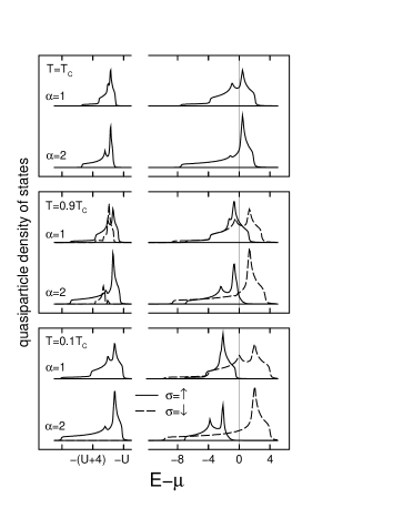
FIG. 4.: Spin-dependent quasiparticle densities of states for the outer and inner layer of a d=3 film. Solid lines: majority spin direction ($\sigma=\uparrow$); broken lines: minority spin direction ($\sigma=\downarrow$). Further parameters: $n=1.4$, $U=48$.

For temperatures below the Curie temperature $T_{C}$ an additional splitting (“exchange-splitting”) in majority ($\sigma=\uparrow$) and minority ($\sigma=\downarrow$) spin direction occurs, leading to non-zero magnetization $m_{\alpha}=n_{\alpha\uparrow}-n_{\alpha\downarrow}$. For $T=0$ the majority QDOS lies completely below the chemical potential, the system is fully polarized ($n_{\alpha\uparrow}=1$). Thus the low-energy subband of the minority spin direction disappears and the minority QDOS is exactly given by the BDOS of the non-interacting system (Fig. 1) due to vanishing correlation effects in the $\sigma=\downarrow$ channel. The reduced surface magnetization at $T=0$ (see Fig. 2) is, therefore, directly caused by the layer-dependent BDOS.

We like to stress that the spin-splitting does not depend on the size of the Coulomb interaction $U$ as long as $U$ is chosen from the strong coupling limit. Contrary to Hartree-Fock theory the spin splitting saturates as a function of $U$ for values of about $2-3$ times the bandwidth of the non-interacting system. The same holds for the Curie temperature $T_{C}$ [44].

The temperature behavior of the QDOS is governed by two correlation effects (Fig. 4). As the temperature is increased, the spin-splitting between $\sigma=\uparrow$ and $\sigma=\downarrow$ spectrum decreases. This effect is accompanied by a redistribution of spectral weight between the lower and upper subbands along with a change of the widths of the subbands. For $T=0.9\,T_{C}$ one clearly sees that in the minority spectrum weight has been transferred from the upper to lower subband which has reappeared due to non-saturated magnetization at finite temperatures. In the $\sigma=\uparrow$ spectrum the opposite behavior is found. For all $T<T_{C}$ the spin splitting is significantly larger in the inner layer compared with the surface. At $T=T_{C}$ the exchange splitting has disappeared whereas the correlation-induced Hubbard splitting is still present.

Let us consider the question why the surface magnetization shows a tendency towards a reduced Curie temperature as seen in Fig. 2. This effect can be understood by the above mentioned moment analysis of the BDOS (Fig. 1): From bulk systems it is known that an asymmetrically shaped BDOS is favorable for the stability of ferromagnetism in the Hubbard model. In particular, the Curie temperatures increase with increasing skewness of the BDOS [42]. The same trend shows up in the present film-system where the skewness of the BDOS is higher for the inner layers compared to the surface-layer. Note that this argument is somewhat more delicate than in the case of Heisenberg films where the reduced surface magnetization is directly caused by the reduced number of interacting sites.

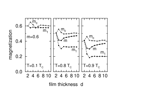
FIG. 5.: Surface-layer magnetization $m_{1}$, central layer magnetization $m_{c}$ and mean magnetization $m$ as a function of the film thickness $d$ and for three reduced temperatures $T/T_{C}=0.1,\,0.8,\,0.9$. Further parameters: $n=1.4$, $U=48$.

In Fig. 5 the difference between surface magnetization $m_{1}$, central-layer magnetization $m_{c}$, and mean magnetization $m$ is analyzed in more detail. For all film thicknesses where this distinction is meaningful ($d\geq 3$), the surface magnetization is reduced with respect to the mean magnetization. This holds not only for very thin films ($d=3-5$, see also Fig. 2) where some oscillations are present that are caused by the finite film thickness, but also extends to the limit $d\rightarrow\infty$ where the two surfaces are well separated and do not interact. The surface and central-layer magnetizations already stabilize for thicknesses around $d=6$. Further, Fig. 5 clearly shows that the reduction of $m_{1}$ drastically increases for higher temperatures. For $T=0.9\,T_{C}$ the surface magnetization is reduced to about half the size of the magnetization in the center of the film.

The charge transfer due to differing layer occupations $n_{\alpha}=n_{\alpha\uparrow}+n_{\alpha\downarrow}$ is found to be smaller than $\approx 0.03$ at $T=0$ and is almost negligible for finite temperatures.

We now like to focus on the magnetic anisotropy energy within the model system (3). The second-order anisotropy constant $K_{2}=K_{2,\text{so}}+K_{2,\text{dip}}$ is calculated via Eq. (12) which needs as an input the temperature-dependent layer magnetizations of the Hubbard film. The dipole constants $\Phi_{\alpha}$ for an fcc(100) film geometry are found to be: $\Phi_{0}=0.7624\cdot 4\pi/3$, $\Phi_{1}=0.1206\cdot 4\pi/3$, $\Phi_{2}=-0.0020\cdot 4\pi/3$, and are set to zero for $\alpha\geq 3$.

To simulate both, surface and volume contribution of the spin-orbit induced anisotropy, we choose the effective anisotropy field (8) in the surface-layer to be different from its value in the volume of the film:

$$\beta_{\alpha}=\left\{\begin{array}[]{ll}\beta_{S}&\textrm{for }\alpha=1,d\\ \beta_{V}&\textrm{else.}\end{array}\right.$$ (21)

In the perturbational approach only the ratio $\beta_{\alpha}/\omega_{0}$ is important. Thus we are left with only two parameters (fixed at $T=0$) to model the RT.

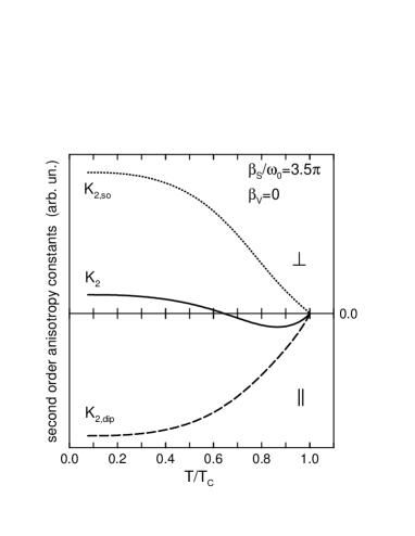
FIG. 6.: Second-order anisotropy constants for a three-layer film in the Fe-type configuration as a function of the reduced temperature $T/T_{C}$. Further parameters: $n=1.4$, $U=48$.

In principle these constants could be taken from experiment or from theoretical ground-state calculations. In our opinion, however, this would mean to somewhat over-judge the underlying rather idealized model system. We are mainly interested in the question whether a realistic temperature-driven RT is possible at all in the Hubbard film and by what mechanism it is induced. Therefore, we choose the parameters $\beta_{S}$ and $\beta_{V}$ conveniently, guided however by the experimental findings in the Fe-type and Ni-type scenarios described in the Introduction.

Fig. 6 and Fig. 7 show that for appropriate parameters $\beta_{S},\,\beta_{V}$ both types of temperature-driven RT can be found within a three-layer film. The same is found for any film thickness $d\geq 3$.

In the Fe-type situation (Fig. 6) we consider a strong positive surface anisotropy field $\beta_{S}/\omega_{0}=3.5\pi$ together with $\beta_{V}=0$. At low temperatures the system is magnetized in out-of-plane direction. As the temperature increases, $K_{2,\text{so}}$ decreases faster than $-K_{2,\text{dip}}$ because of the strong reduction of the surface anisotropy and the magnetization switches to an in-plane position. In principle this kind of RT is possible for all film thicknesses $d\geq 3$. For thicker films $\beta_{S}$ has to be rescaled proportional to $d$ to compensate the increasing importance of the dipole anisotropy.

FIG. 7.: Second-order anisotropy constants for a three-layer film in the Ni-type configuration as a function of the reduced temperature $T/T_{C}$. Further parameters: $n=1.4$, $U=48$.

The Ni-type RT from in-plane to out-of-plane magnetization for a three layer system is obtained by a positive volume anisotropy field $\beta_{V}=6\pi$ and a negative surface anisotropy $\beta_{S}=-0.6\pi$. At low temperatures the dipole anisotropy as well as the negative surface anisotropy field lead to an in-plane magnetization. For higher temperatures, however, where the surface anisotropy becomes less important because of the reduced surface magnetization, the positive volume anisotropy field forces the magnetization to switch to an out-of-plane direction. The ratio $\beta_{S}/\beta_{V}$ determines for what thickness $d$ this type of temperature-driven RT is possible and scales like $\beta_{S}/\beta_{V}\sim 1/d$ for thicker films.

Note that for both types of RT the values of $\beta_{S}$ and $\beta_{V}$ are chosen in such a way that the system is close to a thickness-driven RT. In both cases the RT is mediated by the strong decrease of the surface-layer magnetization compared to the inner layers as a function of temperature.

Finally, we consider the dependence on the band occupation $n$. In Fig. 8 the ratio $m_{1}/m_{c}$ of a three-layer film is plotted as a function of the reduced temperature $T/T_{C}$ for different band occupations $1.4\leq n\leq 1.7$. Above $n=1.78$ and below $n=1.0$ the fcc(100) Hubbard film does not have ferromagnetic solutions whereas between $n=1.0$ and $n=1.3$ there is a tendency towards first order phase transition as a function of temperature[47] and no realistic RT is possible.

FIG. 8.: Ratio $m_{1}/m_{c}$ between surface- and center-layer magnetization as a function of the reduced temperature $T/T_{C}$ for a three-layer film and different band occupations n. In addition $m_{1}/m_{c}$ calculated within Hartree-Fock theory is shown for $n=1.4$. Further parameter: $U=48$.

The ratio $m_{1}/m_{c}$ (Fig. 8) decreases as a function of temperature for all band occupations. For $n=1.4$ which has been considered in Fig. 6 and Fig. 7, it changes from $m_{1}/m_{c}=0.9$ at $T=0$ to $m_{1}/m_{c}=0.4$ close to $T_{C}$. However, for higher band occupations this strong temperature-dependent change in $m_{1}/m_{c}$ diminishes. From the discussion above it is clear that this is unfavorable for the RT. We can thus conclude from Fig. 8 that the possibility of a temperature-driven RT sensitively depends on the band occupation $n$. In addition we plotted in Fig. 8 the ratio $m_{1}/m_{c}$ calculated within Hartree-Fock theory. The result is completely different. At low temperatures we find $m_{1}/m_{c}<1$ whereas $m_{1}/m_{c}>1$ close to $T_{C}$. Note that the ratio $m_{1}/m_{c}$ is almost constant for the wide temperature range $0.1<T/T_{C}<0.9$. Therefore, a realistic temperature-driven RT is excluded within the Hartree-Fock approximation. This holds for all parameters that have been considered here.

VI conclusion

We have applied a generalization of the spectral-density approach (SDA) to thin Hubbard films. The SDA which reproduces the exact results of the $t/U$-perturbation theory in the strong coupling limit, leads to rather convincing results concerning the magnetic properties. The magnetic behavior of the itinerant-electron film can be microscopically understood by means of the temperature-dependent electronic structure.

For an fcc(100) film geometry the layer-dependent magnetizations have been discussed as a function of temperature as well as film thickness. The magnetization in the surface layer is found to be reduced with respect to the inner layers for all thicknesses and temperatures. By analyzing the layer-dependent QDOS this reduction can be explained by the fact that in the free BDOS both variance and skewness are diminished in the surface-layer compared to the inner layers.

The inclusion of the dipole interaction and an effective layer-dependent anisotropy field allows to study the temperature-driven RT. The second-order anisotropy constants have been calculated within a perturbational approach. For appropriate strengths of the surface and volume anisotropy fields both types of RT, from out-of-plane to in-plane (Fe-type) and from in-plane to out-of-plane (Ni-type) magnetization are found. For the Ni-type scenario the inclusion of a positive volume anisotropy is necessary. The RT in our itinerant model system is mediated by a strong reduction of the surface magnetization with respect to the inner layers as a function of temperature. Here a close similarity to the model calculations within Heisenberg-type systems is apparent, despite the fact that these models completely ignore the itinerant nature of the magnetic moments in the underlying transition-metal samples. Contrary to Heisenberg films, the band occupation $n$ enters as an additional parameter within an itinerant-electron model. We find that the possibility of a RT sensitively depends on the band occupation. The fact that no realistic RT is possible within Hartree-Fock theory clearly points out the importance of a reasonable treatment of electron correlation effects.

- [1] M. L. Néel, J. Phys. Radium 15, 225 (1954).
- [2] D. P. Pappas, K.-P. Kämper, and H. Hopster, Phys. Rev. Lett. 64, 3179 (1990).
- [3] D. P. Pappas, C. R. Brundle, and H. Hopster, Phys. Rev. B 45, 8169 (1992).
- [4] Z. Q. Qiu, J. Pearson, and S. D. Bader, Phys. Rev. Lett. 70, 1006 (1993).
- [5] R. Allenspach, M. Stampanoni, and A. Bischof, Phys. Rev. Lett. 65, 3344 (1990).
- [6] R. Allenspach and A. Bischof, Phys. Rev. Lett. 69, 3385 (1992).
- [7] R. Allenspach, J. Magn. Magn. Mat. 129, 160 (1994).
- [8] H. Fritzsche, J. Kohlhepp, H. J. Elmers, and U. Gradmann, Phys. Rev. B 49, 15665 (1994).
- [9] D. E. Fowler and J. V. Barth, Phys. Rev. B 53, 5563 (1996).
- [10] M.-T. Lin, J. Shen, W. Kuch, H. Jenniches, M. Klaua, C. M. Schneider, and J. Kirschner, Phys. Rev. B 55, 5886 (1997).
- [11] B. Schulz and K. Baberschke, Phys. Rev. B 50, 13467 (1994).
- [12] K. Baberschke, Appl. Phys. A 62, 417 (1996).
- [13] A. Braun, B. Feldmann, and M. Wuttig, J. Magn. Magn. Mat. 171, 16 (1997).
- [14] M. Farle, W. Platow, A. N. Anisimov, P. Poulopoulos, and K. Baberschke, Phys. Rev. B 56, 5100 (1997).
- [15] M. Farle, W. Platow, A. N. Anisimov, B. Schultz, and K. Baberschke, J. Magn. Magn. Mat. 165, 74 (1997).
- [16] H. Takayama, K.-P. Bohnen, and P. Fulde, Phys. Rev. B 14, 2282 (1976).
- [17] P. Bruno, Phys. Rev. B 39, 865 (1989).
- [18] M. Cinal, D. M. Edwards, and J. Mathon, Phys. Rev. B 50, 3754 (1994).
- [19] A. Lessard, T. H. Moos, and W. Hübener, Phys. Rev. B 56, 2594 (1997).
- [20] Ding sheng Wang, Ruqian Wu, and A. J. Freemann, Phys. Rev. B 47, 14932 (1993).
- [21] G. H. O. Daalderop, P. J. Kelly, and M. F. H. Schuurmans, Phys. Rev. B 50, 9989 (1994).
- [22] R. Lorenz and J. Hafner, Phys. Rev. B 54, 15937 (1996).
- [23] O. Hjortstam, K. Baberschke, J. M. Wills, B. Johansson, and O. Eriksson, Phys. Rev. B 55, 15026 (1997).
- [24] A. B. Shick, D. L. Novikov, and A. J. Freemann, Phys. Rev. B 56, 14259 (1997).
- [25] H. B. Callen and E. Callen, J. Phys. Chem. Solids 27, 1271 (1966).
- [26] L. M. Levinson, M. Luban, and S. Shtrikman, Phys. Rev. 187, 715 (1969).
- [27] D. Pescia and V. L. Pokrovsky, Phys. Rev. Lett. 65, 2599 (1990).
- [28] P. J. Jensen and K. H. Bennemann, Phys. Rev. B 42, 849 (1990).
- [29] P. J. Jensen and K. H. Bennemann, Solid State Commun. 100, 585 (1996).
- [30] P. J. Jensen, Acta. Phys. Polonia A 92, 427 (1997).
- [31] A. Moschel and K. D. Usadel, Phys. Rev. B 51, 16111 (1995).
- [32] A. Moschel and K. D. Usadel, J. Magn. Magn. Mat. 140-144, 649 (1995).
- [33] A. Hucht and K. D. Usadel, Phys. Rev. B 55, 12309 (1997).
- [34] A. B. MacIsaac, J. P. Whitehead, K. De’Bell, and P. H. Poole, Phys. Rev. Lett. 77, 739 (1996).
- [35] A. B. MacIsaac, K. De’Bell, and J. P. Whitehead, Phys. Rev. Lett. 80, 616 (1998).
- [36] Y. Millev and J. Kirschner, Phys. Rev. B 54, 4137 (1996).
- [37] J. Hubbard, Proc. R. Soc. London, Ser. A 276, 238 (1963).
- [38] M. Ulmke, Euro. Phys. J. B 1, 301 (1998).
- [39] D. Vollhardt, N. Blümer, K. Held, J. Schlipf, and M. Ulmke, Z. Phys. B 103, 283 (1997).
- [40] M. P. Gokhale and D. L. Mills, Phys. Rev. B 49, 3880 (1994).
- [41] M. Plihal and D. L. Mills, Phys. Rev. B 52, 12813 (1995).
- [42] J. Wahle, N. Blümer, J. Schlipf, K. Held, and D. Vollhardt, preprint (1998).
- [43] W. Nolting and W. Borgieł, Phys. Rev. B 39, 6962 (1989).
- [44] T. Herrmann and W. Nolting, J. Magn. Magn. Mat. 170, 253 (1997).
- [45] A. B. Harris and R. V. Lange, Phys. Rev. 157, 295 (1967).
- [46] H. Eskes and A. M. Oleś, Phys. Rev. Lett. 73, 1279 (1994).
- [47] T. Herrmann and W. Nolting, Solid State Commun. 103, 351 (1997).
- [48] M. Potthoff, T. Herrmann, T. Wegner, and W. Nolting, preprint (1998).
- [49] W. Nolting, W. Borgieł, V. Dose, and Th. Fauster, Phys. Rev. B 40, 5015 (1989).
- [50] W. Nolting, A. Vega, and Th. Fauster, Z. Phys. B 96, 357 (1995).
- [51] A. Vega and W.Nolting, phys. stat. sol. (b) 193, 177 (1996).
- [52] M. Potthoff and W. Nolting, J. Phys.: Condens. Matter 8, 4937 (1996).
- [53] M. Potthoff and W. Nolting, Surf. Sci. 377-379, 457 (1997).
- [54] M. Potthoff and W. Nolting, Z. Phys. B 104, 265 (1997).
- [55] T. Herrmann and W. Nolting, Phys. Rev. B 53, 10579 (1996).
- [56] W. Nolting and T. Herrmann, preprint (1998).
- [57] T. Herrmann and W. Nolting, to be published (1998).