Transmission and Scattering of a Lorentz Gas on a Slab

Abstract

We perform numerical scattering experiments on a Lorentz array of disks centered on a triangular lattice with $L$ columns and study its transmission and reflection properties. In the finite horizon case, the motion of the particles may be modeled as simple one dimensional random walks with absorbing walls for which the scaling of the transmission and reflection coefficients are known, and agree with those found numerically. In the infinite horizon case the analogy with a simple diffusive process is no longer valid. In this case we compare our results to those expected for a one dimensional Lévy walk, again with absorbing walls, for which logarithmic corrections to the scaling relations appear. These corrections are consistent with the numerical results. The scaling with $L$ and the symmetry properties of the forward $\sigma_{T}(\phi)$ and backward $\sigma_{R}(\phi)$ differential cross sections are also studied, and some of their salient features are discussed.

PACS number(s): 05.40 +j,05.45 +b,05.60 +w

I Introduction

The Lorentz gas is an ensemble of noninteracting point particles which move freely with elastic reflections from fixed scatterers [3]. It is a basic model for linearized kinetic equations [4] and its ergodic properties are well known [5].

In this paper we present the results of numerical experiments in which a large number of particles are incident on an array of disks centered on a triangular lattice. The particles are launched initially either in the $+x$ direction or isotropically towards the array, and are reflected elastically from the scatterers. The array of disks is finite in the $x$ direction and infinite in the $y$ direction so we speak of a “slab” of scatterers. Our slab is characterized by two parameters, the width of the slab, that is, the number $L$ of columns of scatterers, and the separation $w$ between them (the disk radius is unity). The quantities that are measured are the transmission $T$ and reflection $R$ coefficients, the mean survival time $\tau$ of particles in the slab and the transmitted $\sigma_{T}$ and reflected $\sigma_{R}$ differential cross sections. These quantities are analyzed as functions of the parameters characterizing the slab.

If the separation between scatterers $w$ in a triangular lattice is small, $w<w_{c}=0.3094\dots$, the length of free motion of the point particles is bounded, that is, the particles “see” a finite horizon. On the other hand, when $w_{c}<w$ the length of free motion may be unbounded, the particles “see” an infinite horizon. In this work we study the scattering properties in both situations, and analyze our results in terms of the characteristic motion of the particles in each case. In the finite horizon case, the motion of the particles is known to be diffusive [6] and the diffusion coefficient can be estimated with ergodic arguments [7]. Velocity correlation functions have been shown to decay exponentially [6], as confirmed by numerical experiments [8]. In contrast, for the infinite horizon case the diffusion coefficient diverges logarithmically [9, 10] and correlation functions have a power law decay [11]. We find that there are also fundamental differences in the scattering properties for each case.

Lorentz gases in finite size geometries have also been introduced elsewhere with the aim of studying escape rates and their relation to transport coefficients and fractal repellers [12]. An account of these results, together with a formulation of the problem in terms of flux boundary conditions can be found in Ref. [13].

In Section II we introduce all the definitions and discuss in detail the numerical experiments for the case of a finite horizon. Section III draws an analogy between the Lorentz scattering experiments in the finite horizon case and the behavior of one-dimensional diffusive motion with absorbing boundaries. This serves as a basis for the explanation of the observed scaling laws for transmission coefficients and survival times. In Section IV we present the results for the infinite horizon case when the particles are launched initially in the $x$ direction. These show logarithmic corrections to the scaling laws, which are consistent with considering the motion of the particles within the slab as a Lévy walk. In Section V we discuss angular dependences and symmetries of the transmission and reflection differential cross sections. In Section VI we discuss how some of the scattering properties are affected by sending the particles isotropically, i.e. with an incidence angle uniformly distributed between $-\pi/2$ and $\pi/2$. A modified random walk model displaying these same differences is also briefly discussed. Finally, Section VII is devoted to discussion of the results and conclusions.

II Scattering with a finite horizon

The scatterers we consider are disks of unitary radius centered on a triangular lattice as shown in Fig. 1. The distance between neighboring centers is $2+w$ and the centers lie along $L$ lines parallel to the $y$ axis. The slab is finite in the $x$ direction and infinite in the $y$ direction. A large number $N$ of particles are incident from the left parallel to the $x$ axis with unit speed. The particles move freely except for elastic collisions at the boundary of the disks. In the experiments, the dynamics is solved by considering the motion in the elementary Wigner-Seitz hexagonal cell where opposite sides are identified. Each incident particle has a different impact parameter $b$, defined here as the distance between the initial position and the horizontal line passing through the center of the scatterer in the Wigner-Seitz cell. Due to the symmetry of the slab, it is sufficient to consider b between 0 and $1+w/2$. The trajectory in the slab is obtained by unfolding the orbit in the Wigner-Seitz cell. The cases where particles are incident with an angle different from zero and the effect of isotropic incidence will be briefly discussed in Section VI.

FIG. 1.: Slabs of scatterers in a triangular array. (a) Finite horizon, $w=0.3$, with $L=5$. (b) Infinite horizon, $w=1.$, with $L=5$.

In the finite horizon case, $0<w<w_{c}=(4/\sqrt{3}-2)=0.3094\dots$, the particles that enter the scatterer cannot travel long distances without suffering collisions. In the infinite horizon case, $w_{c}<w$, the particles may travel arbitrarily far between collisions, due to the opening of infinite corridors. If $w_{c}<w<2$ the infinite corridors lie at angles of $\pi/6$, $\pi/3$, and $\pi/2$. We will be mainly considering particles incident parallel to the $x$ axis that cannot cross the slab without collisions when $w<2$.

Since the slab is infinite in the $y$ direction and the collisions are elastic, every particle that enters the slab must eventually exit it, except for a set of measure zero which goes asymptotically to periodic orbits inside the slab (we disregard all zero measure sets herafter). Thus, in practice, a particle that enters the slab collides with some of the obstacles and will be ultimately transmitted or reflected, leaving the slab with an angle $\phi$ measured with respect to the $+x$ direction. Particles are transmitted if they exit the slab from the right ($|\phi|<\pi/2$), and are reflected if they exit from the left ($|\phi|>\pi/2$).

A first characterization of the system is through the computation of the transmision $T$, and reflection $R$, coefficients. The former is defined as the fraction of particles that pass through the slab and exit on the right, and the latter as the particle fraction that exits the slab on the left (obviously $T+R=1$). A finer quantity is the differential scattering cross section $\sigma$ defined by saying that $\sigma(\phi)d\phi$ is the fraction of particles scattered between $\phi$ and $\phi+d\phi$. We can separate this quantity in the transmitted $\sigma_{T}$ and reflected $\sigma_{R}$ differential scattering cross sections by considering $|\phi|<\pi/2$ and $|\phi|>\pi/2$ respectively.

In Fig. 2 we show the dependence of the transmission coefficient $T$ on $L$ for the finite horizon case. These results are consistent with the scaling law $T\sim L^{-\beta}$ where $\beta\approx 1$ independently of $w$. This behavior will be justified in the next section drawing from an analogy with random walks. Since $R=1-T$ and $T$ scales to zero with $L$, $R$ does not depend on $L$ for $L\gg 1$. Another quantity of interest is the mean survival time inside the slab $\tau$. This average time is evaluated over all the $N$ incident particles no matter if they are transmitted or reflected. We find that $\tau\sim L^{\gamma}$ with $\gamma\approx 1$ as we show in Fig. 3.

III Diffusive behavior in finite size systems

In the finite horizon case, rigorous results, convincing evidence and plausible arguments have been set forth indicating that the motion of the particles in the Lorentz system can be accurately modeled as a simple random walk [6, 7]. In its simplest version the particles can be viewed as hopping between adjacent “cages” in an essentially uncorrelated fashion, and staying in each cage for a well defined average time. For the case under study in this paper it is not even necessary to consider the random walk process as occuring on a two dimensional lattice since the quantities we are interested in can be calculated from the projection of the walk onto the finite direction $x$.

While the discrete one dimensional random walk on a finite lattice can be described completely [14, 15], such a detailed comparison between the two systems cannot hold. As the random walk is an analogy to the Lorentz system, the best we can realistically expect to determine from it is the scaling behavior of the quantities under study. With this in mind, we choose to evaluate the transmission and reflection coefficients for the simple random walk problem via the diffusion equation, with a numerically determined phenomenological diffusion constant $D$. This equation describes the evolution of the coarse grained particle density in the system and is expected to be valid when the system size is much greater than the root mean square (rms) step length. Once again, since the slab is translationally invariant along the $y$ axis, the coarse grained particle density obeys a diffusion equation along $x$.

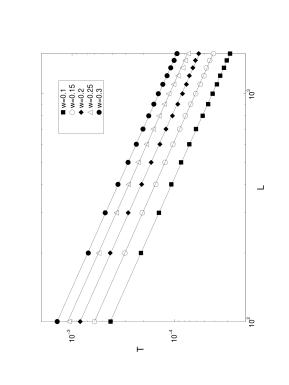
FIG. 2.: Logarithmic plot of the transmission coefficient T as a function of the size of the system L, for different values of $w$. The number N of incident particles were, for $w=0.1,4\times 10^{7}$; for $w=0.15,2\times 10^{7}$, and for $w=0.2,0.25,0.3,10^{7}$. The full lines are the least square fits, all of them compatible with the theoretical prediction $T\sim L^{-1}$ to within $1\%$.

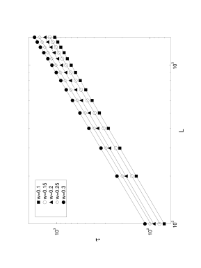
FIG. 3.: Logarithmic plot of the survival time $\tau$ vs. $L$ for the same values of $w$ and $N$ as in Fig. 2. The full lines are the least square fits, all of them compatible with the theoretical prediction $\tau\sim L$ to within $1.6\%$.

To estimate the reflection and transmission coefficients within this approximation, we require the solution of the diffusion equation with absorbing boundary conditions at $x=0$ and $x=X$ and a constant unit input flux at site $a$. In the steady state, the magnitude of the fluxes at 0 and $X$ will give the splitting probabilities; i.e. the probability that a particle injected at position $a$ will be absorbed at the origin or at $X$. In our scattering system the particles are inciding on the left, which can be thought of as having the injection point $a$ near the origin. Then the calculation outlined above yields the transmission coefficient

$$T=a/X.$$ (1)

To estimate the mean survival time of the particles within the slab, we recall that within the diffusion approximation, the survival time for a random walker starting at position $a$ satisfies the equation [15]

$$D{d^{2}\tau(a)\over da^{2}}=-1~{},$$ (2)

with the conditions $\tau(0)=\tau(X)=0$, where $D$ is again the diffusion constant of the process. Thus

$$\tau(a)={1\over 2D}a(X-a)~{},$$ (3)

and if the injection point is taken to be close to the origin ($a\ll X$), we obtain

$$\tau\sim aX/2D.$$ (4)

These results can also be obtained on a more general footing through Wald’s identity  [15], and are expected to hold as long as the rms step size of the random walk is small compared to the system size $X$, and the number of steps given by the random walker scales linearly with time (i.e. there are no long tail waiting time distributions).

We can identify the quantities appearing in Eqs. (1) and (4) corresponding to the Lorentz scattering experiment. The diffusion coefficient $D$ is computed in Ref. [7] in a random walk approximation and numerically through the Green-Kubo relation. The length $X$ is related to $w$ and $L$ by $X=L(2+w)\sqrt{3}/2$ and thus the penetration length $a$ can be determined by the slope of the dependence of $\tau$ on $L$ as in Fig. 3. The results are consistent with the distance between traps $(2+w)/\sqrt{3}$, as defined in Ref. [7], for small values of $w$ (where also the diffusion constant predicted in the random walk approximation agrees with the numerically determined one).

IV Infinite horizon

When the horizon becomes infinite the analogy to the simple diffusive process breaks down. This occurs as a consequence of the opening of infinite corridors between scatterers in which the particle is capable of travelling very large distances between collisions. The distribution of the length of these sojourns, $p(r)$, has been shown to decay as $r^{-3}$ when $r\to\infty$ by both numerical results and theoretical arguments [9, 16, 10, 17]. Thus the rms step length diverges and the diffusive approximation described in the last section breaks down.

If we insist on making a random walk description of the system, we are now led to consider a random walk with a distribution of step lengths without second moment (generically called “Lévy flights”  [15, 18]). Here one sometimes makes the distinction between a discrete time process, in which each step is selected from a power-law distribution of lengths, but always takes a fixed time and the so-called Lévy walk in which each step takes a time proportional to its length. This latter, while more relevant to the case we are discussing, is not significantly different from the Lévy flight if the first moment of the step size distribution exists, as it certainly does in our case. We shall therefore ignore the considerable complications this causes and often identify time with the number of jumps or collisions $n$.

In contrast to the diffusive case, the derivation of the transmission coefficient in the case of Lévy flights appears not to have been treated in the literature. We present an argument which leads to a scaling prediction which seems reasonable for general Lévy flights, and specialize it to the case we are concerned with.

Denote the step distribution of the Lévy flight as $P(r)\sim 1/|r|^{1+\alpha}$ with $0<\alpha\leq 2$. A random walker with this step distribution travels a typical distance [18]

$$\xi^{2}\sim\cases{t^{2/\alpha}&{\rm for} $1<\alpha<2$\cr t\ln t&{\rm for} $\alpha=2$\cr t&{\rm for} $\alpha>2$\cr}$$

in time t.

If we assume that the particle is initially at a point $a$ sufficiently near the origin ($a\ll X$), then we can invoke Sparre-Andersen’s theorem [14]. This theorem states that the probability that the walker steps for the first time to the left of the point $a$ at the $n$-th step is a universal function $\pi(n)$, which is completely independent of any of the properties of $P(r)$, as long as $P(r)$ is symmetric and continuous. This distribution is found to decay as $\pi(n)\sim n^{-3/2}$ for any kind of unbiased walk whatsoever, in particular for the Lévy flights we are concerned with. This allows us to estimate straightforwardly the behaviour of Lévy flights both as regards their transmission and the mean survival time in the interval considered.

The scaling behavior of the transmission coefficient of a Lévy walk across a finite system of length $X$ can be estimated as follows: Denote by $\tau_{\alpha}(X)$ the time required for the walker to travel a distance of order $X$ with appreciable probability. The transmission coefficient is then the probability that the walker never steps left of the origin during $\tau_{\alpha}(X)$. From the above scaling relation, $\tau_{\alpha}(X)$ is expected to scale as $X^{\alpha}$ for $1<\alpha<2$, as $X^{2}/\ln X$ for $\alpha=2$ and as $X^{2}$ for $\alpha>2$, which corresponds to normal diffusion. Then, in terms of $\tau_{\alpha}(X)$ the transmission coeficient is given by

$$T(X)\sim\sum_{n\geq\tau_{\alpha}(X)}^{\infty}\pi(n)\sim\int_{\tau_{\alpha}(X)}^{\infty}t^{-3/2}dt\sim 1/\sqrt{\tau_{\alpha}(X)}.$$ (5)

For $\alpha>2$ we therefore get the behavior of the ordinary diffusive case treated in Section III. In particular, for our infinite horizon Lorentz slab, we expect $T(X)\sim{\sqrt{\ln L}}/L$.

As for the survival time, it is estimated in a similar way: The probability of leaving the interval $[0,X]$ at time $n$ is given by $\pi(n)$ as long as $n$ is not so large that leaving at the right hand-side becomes appreciably likely. This occurs at times of the order of $\tau_{\alpha}(X)$. This reasoning gives for the mean first exit time $\tau$

$$\tau\sim\sum_{n=1}^{\tau_{\alpha}(X)}n\pi(n)\sim\sqrt{\tau_{\alpha}(X)}.$$ (6)

The prediction for the probability distribution $\pi(n)$ of leaving the slab to the left after $n$ collisions based on the Sparre-Andersen theorem can be tested for the Lorentz gas; it is valid both for the finite horizon case and for the infinite horizon. In Fig. 4 we show this distribution as obtained from the simulation for $w=1.5$ (infinite horizon) together with the Sparre-Andersen scaling law. The agreement is good even for small values of $n$.

FIG. 4.: The probability distribution $\pi(n)$ of leaving the system to the left after $n$ collisions, for $w=1.5$, and from left to right $L=100,500,1000,1500$ and $N=10^{7}$. The Sparre-Andersen scaling result is shown by the dashed lines.

The scaling laws for the transmission coefficient and for the mean survival time can be also tested for the Lorentz gas in the infinite horizon case. In Fig. 5 we show $(TL)^{2}$ for a set of $w$ values as a function of $\ln(L)$. According to our theory $(TL)^{2}\sim\ln(L)$ for $w_{c}<w$. In Fig.6 we show $(\tau/L)^{2}$ as a function of $\ln(L)$ in order put in evidence the predicted logarithmic correction.

Runs were also carried out at other fixed incidence angles, and the same features as described above were obtained. We have thus shown that, given a fixed angle incidence, the opening of the horizon appears to produce logarithmic corrections to the scaling laws present for finite horizon. This feature is shared by the behavior of other quantities which also present logarithmic corrections, such as the diffusion coefficient.

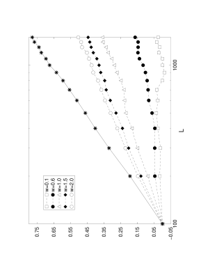
FIG. 5.: The logarithmic correction to $T$ is shown by plotting $[(LT(L))^{2}-(100T(100))^{2}]/(100T(100))^{2}$ vs. $\ln(L)$ for $w=0.1$ (with $N=4\times 10^{7}$), and $w=0.6,1.0,1.5,2.0$ (with $N=10^{7}$). Straight lines with nonzero slope, indicating the logarithmic correction, are expected for $w$ above the infinite horizon. The dotted lines are meant as a guide to the eye.

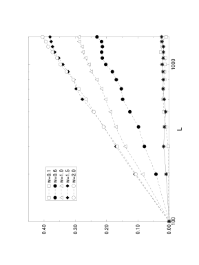
FIG. 6.: The logarithmic correction to $\tau$ is shown by plotting $[(L/\tau(L))^{2})-(100/\tau(100))^{2}]/(100/\tau(100))^{2}$ vs $\ln(L)$ for the same values of $w$ and $N$ as in Fig. 5. Again straight lines with nonzero slope are expected for $w$ above the infinite horizon, and we also show the corresponding quantity por a Lévy walk with $\alpha=2.0$. The dotted lines are meant as a guide to the eye.

V Angular Dependence of Forward and Backward Scattering

We have already observed that for fixed incidence angle the transmission coefficient scales as $1/L$ in the finite horizon case, whereas it scales as $\sqrt{\ln L}/L$ in the case of infinite horizon. It is also instructive to look in somewhat greater detail at the angular distribution of the transmitted and reflected particles (this is what is done also in chaotic scattering experiments with fewer scatterers [19]). We define $\sigma_{R}(\phi)$ as the density of particles reflected at angle $\phi$ and $\sigma_{T}(\phi)$ similarly for the transmitted particles. Due to the symmetry $\phi\to-\phi$ the range of $\phi$ will be from 0 to $\pi/2$ for transmitted particles and from $\pi/2$ to $\pi$ for those that are reflected. As these distributions are also dependent on $L$, we further propose that in the finite horizon case they can be expanded as

$$\sigma_{R}(\phi)=a_{R}(\phi)+{b_{R}(\phi)\over L}+\cdots$$ (7)

and

$$\sigma_{T}(\phi)={b_{T}(\phi)\over L}+\cdots.$$ (8)

The leading term in the transmission cross section is zero since there is no transmission for infinite $L$. The following relation has then been found to hold in all cases for sufficiently large $L$ (see Fig. 7):

$$b_{R}(\phi)=-b_{T}(\pi-\phi)$$ (9)

This symmetry relation can be understood as follows: Imagine that the slab is subjected to a continuous flow of particles with identical distributions incident from both sides of the sample. If we now look at the distribution of angles of the particles which go to the right in these circumstances, it is given by the superposition $\sigma_{T}(\phi)+\sigma_{R}(\phi)=a_{R}(\phi)+{b_{R}(\phi)\over L}+{b_{T}(\phi)\over L}+\cdots$. Now, by symmetry, the above set-up is equivalent to having particles incident only from the right and a reflecting wall at the middle of the sample. However, from the fact that a particle travelling deep into the slab eventually loses memory of its original incidence direction, it follows that the trajectory of a particle reflected on the wall is indistinguishable with the trajectory of a particle travelling in a semi-infinite system and eventually returning across the position of the wall (which occurs with probability one). Thus, given that the correlation with the initial incidence is small enough, the system with the reflecting wall will not show any great difference from the semi-infinite system ($L=\infty$) as far as the angular distribution of its particles is concerned. This then allows to derive the identity

$$a_{R}(\phi)=a_{R}(\phi)+{b_{R}(\phi)+b_{T}(\pi-\phi)\over L}+\cdots$$ (10)

from which the result follows. Numerically, this is quite well borne out both in the case of finite (Fig. 7) and infinite horizon (Fig. 8).

FIG. 7.: The quantities $b_{T}(\phi/\pi)$ ($\bullet$) and $b_{R}((\pi-\phi)/\pi)$ ($\bigtriangleup$) vs. $\phi/\pi$ for $w=0.3$ and $N=10^{7}$. The values for $b_{T}$ are extracted from data with $L=100$ and those for $b_{R}$ are determined by substraction of data with $L=200$ and $L=100$.

FIG. 8.: The quantities $-b_{T}(\phi/\pi)$ ($\bullet$) and $b_{R}((\pi-\phi)/\pi)$ ($\bigtriangleup$) vs. $\phi/\pi$ for $w=1.5$ and $N=10^{7}$. The values for $b_{T}$ are extracted from data with $L=100$ and those for $b_{R}$ are determined by substraction of data with $L=200$ and $L=100$.

In the case of infinite horizon, another striking feature of the angular distribution function is found: there is a clear peak in $b_{T}$ around the value $\phi_{c}=\pi/6$ as well as a corresponding dip in $a_{R}$ around the value $\phi_{c}=5\pi/6$ (see Fig.9) which are the angles the infinite corridors make with the edge of the sample. Qualitatively, the appearence of these singularities can be argued as follows. As is well-known, the periodic system corresponding to the one we are studying is ergodic, so that all allowed positions and all directions are eventually equally probable. In the finite system we are studying, this is no longer the case. In particular, near the edges, the relative weight of the directions leading to escape will be different from the other ones. Nevertheless, we may at first start with the approximation that, at least as long as the particles enter reasonably deep into the system, the hypothesis of equidistribution of velocity directions holds to a good approximation. Then we may estimate the transmission coefficient as a function of angle by means of the fraction of surface area from which trajectories escape at that angle (we may assume that the transverse direction of the gas is made finite by some device such as periodic boundary conditions). This yields a singularity in the angular dependence of the transmission coefficient near the critical angles when $L\to\infty$.

FIG. 9.: The quantities $b_{T}$ (full line) and $a_{R}$ (dashed line) vs. $\phi/\pi$ for $w=1.5$, $N=10^{6}$. The features expected at $\phi=\pi/6$ and $\phi=5\pi/6$ are clear. There is also a peak at $\phi\approx{\rm arctan}\sqrt{2}$, for which we have no explanation.

VI The Effect of Isotropic Incidence

The following apparent difficulty motivated us to also study the case in which the particles are isotropically incident upon the slab: In the preceding Section, we reported numerical and theoretical evidence for the existence of a logarithmic correction to the mean survival time. Yet a quite general argument appears to show such a correction is impossible. Consider the phase space on a constant energy shell inside the Lorentz array. The volume of this phase space, which clearly scales as $L$, can be expressed as the integral of the time of residence inside the system over all points of entry (this relation is known as the Katz formula [20]). Since the volume of trajectories that remain forever confined to the system is zero, and the volumes of those entering from the left and from the right are equal, it follows that the mean survival time scales as $L$, in contradiction to what was numerically observed in the last Section, as well as to the predictions of the Lévy flight model.

If we consider the above argument carefully, however, we see that it only applies if all angles of incidence are taken as equally probable. To understand why this might make a difference, one should note the following: If all angles are equally probable, then the distribution of initial step lengths will have a singularity due to the probability of launching the particle with an angle very close to critical and an appropiate impact parameter. This leads, as is readily seen, to the probability for a large initial step length of $x$ going as $x^{-2}$. This behaviour is in marked contrast to the step probability distribution within the interior of the system, for which the impact parameter and the angle are interrelated. For these, as was pointed out before, the probability of a large step $x$ goes as $x^{-3}$.

In order to clarify these issues, we performed simulations on the system with isotropic incidence. Indeed, as expected from the above argument, the mean survival time was found to scale as $L$, without any logarithmic corrections (see Fig. 6). On the other hand, the transmission coefficient was found to retain its peculiar behaviour (see Fig. 5). The above argument is therefore sound, it does not contradict the numerical work reported in the previous Section. On the contrary, since the two models show such clear differences with regard to their mean survival time, this seems to indicate that the distribution of initial step lengths may well have been the cause.

To test this final hypothesis, we also simulated a Lévy walk with $\alpha=2$ in which the first step has a distribution with an $x^{-2}$ tail, corresponding to $\alpha=1$. The results are again very clear: the mean survival time now grows as $L$ without any logarithmic corrections. On the other hand, the transmission coefficient still has the previous anomalous behaviour, though it takes a somewhat longer time to reach it.

VII Concluding remarks

In this work we have examined the scattering properties of a Lorentz gas incident on an array of scatterers centered on a triangular lattice with a finite number $L$ of columns. Much of our attention has focused on the scaling with $L$, for large values of $L$, of transport and optical properties, namely, transmission and reflection coeficients, mean survival time and differential cross section. It should be emphasized that though most of the numerical results reported in this paper were obtained for incidence along the $x$ direction, exactly the same phenomena was observed in runs carried out at other fixed incident angles. On the other hand, some significant differences were found when the particles were launched isotropically in the infinite horizon case.

For our understanding of the observed numerical trends we have considerably profited from the link, in some cases formal, in others qualitative, to random walk processes. Two regimes are considered: the finite and the infinite horizon cases. For finite horizon the transmission coefficient scales with $1/L$, the survival time with $L$ and the differential cross-section has no singularities and presents certain symmetry properties. All this is in agreement with the behavior of normal diffusion and ordinary random walks with absorbing boundaries.

The infinite horizon case, on the other hand, exhibits logarithmic corrections to the aforementioned scalings depending on the incidence angle distribution (in this case the relation to Lévy walks is illuminating). Also, singularities appear in the differential cross section at angles corresponding to the corridors inside the slab, for which we only have a partial understanding. A peculiar effect related to the difference observed between particles launched in one fixed direction and particles launched isotropically can also be explained in terms of a simple Lévy flight model with a different distribution for the initial step length. This allows an explanation for the a discrepancy in the behavior of the mean survival time, which had been anticipated on quite general grounds.

It is also of interest to understand the features of the free motion length distribution. For finite horizon two peaks in such distribution are present at the values $w$ and $\sqrt{3}(2+w)-2$, which correspond to the unstable periodic orbits perpendicular to the disks. For infinite horizon a set of peaks develops, whose number increases with $w$; the slope of the envelope of the probability distribution is $-3$. The origin of such peaks, which most probably are related to other periodic orbits, remains to be analyzed.

REFERENCES

- [1] e-mail: rrs@mazatl.cie.unam.mx
- [2] e-mail: ruffo@ing.unifi.it
- [3] H.A. Lorentz, Proc. Amst. Acad. 7, 438, 585, 604 (1905).
- [4] G. Gallavotti, Phys. Rev. 185, 308 (1969); E.H. Hauge, in Lecture Notes in Physics, 31 pp. 337-367 (1974).
- [5] Sh. Goldstein, J. Lebowitz amd M. Aizenman, in Lecture Notes in Physics, 38 pp. 112-143 (1975); G. Gallavotti, in Lecture Notes in Physics, 38, pp. 236-295 (1975); Ya. G. Sinai, Funkts. Anal. Ego Prilozh., 13, 46 (1979).
- [6] L. A. Bunimovich and Ya. G. Sinai, Commun. Math. Phys. 78, 479 (1981).
- [7] J. Machta and R. Zwanzig, Phys. Rev. Lett. 50, 1959 (1983).
- [8] P.L. Garrido and G. Gallavotti, J. Stat. Phys. 76, 549 (1994).
- [9] J.P. Bouchaud and P. Le Doussal, J. Stat. Phys., 41, 225 (1985).
- [10] P. M. Bleher, J. Stat. Phys., 66, 315 (1992).
- [11] J. Machta, J. Stat. Phys. 32, 555 (1983); B. Friedman and R.F. Martin Jr., Phys. Lett. 105A, 23 (1984).
- [12] P. Gaspard and G. Nicolis, Phys. Rev. Lett., 65, 1693 (1990); P. Gaspard and F. Baras, Phys. Rev. E, 51 5332 (1995).
- [13] P. Gaspard, Physica A, 240, 54 (1997).
- [14] W. Feller, An Introduction to Probability Theory and its Applications, vol. 2, second edition (John Wiley, N.Y.) 1971.
- [15] G.H. Weiss, Aspects and Applications of the Random Walk (North-Holland, Amsterdam) 1994.
- [16] A. Zacherl, T. Geisel, J. Nierwetberg and G. Radons, Phys. Lett. A, 114, 317 (1986).
- [17] P. Dalquist, Nonlinearity, 10, 159 (1997); P. Dalquist and R. Artuso, Phys. Lett A, 219, 212 (1996).
- [18] J.-P. Bouchaud and A. Georges, Phys. Rep., 195, 127 (1990).
- [19] B. Eckhardt, Physica D, 33, 89 (1988).
- [20] I. P. Kornfeld, Y. G. Sinai and S. V. Fomin; Ergodic Theory (Nauka, Moscow) 1980.