Diamagnetic response of a normal-metal–superconductor proximity system at arbitrary impurity concentration

Abstract

We investigate the magnetic response of normal-metal–superconductor proximity systems for arbitrary concentrations of impurities and at arbitrary temperatures. Using the quasiclassical theory of superconductivity a general linear-response formula is derived which yields a non-local current-field relation in terms of the zero-field Green’s functions. Various regimes between clean-limit and dirty-limit response are investigated by analytical methods and by solving the general formula numerically. In the ballistic regime, a finite mean free path reduces the non-locality and leads to a stronger screening than in the clean limit even for a mean free path much larger than the system size. Additionally, the range of the kernel describing the non-locality is strongly temperature-dependent in this case. In the diffusive limit we find a cross-over from local to non-local screening, which restricts the applicability of the dirty-limit theory.

I Introduction

A normal metal in good metallic contact to a superconductor acquires induced superconducting properties. The basic features of this proximity effect were already well understood in the sixties. One of these properties is the diamagnetic screening of an applied magnetic field, which has been studied in a series of experimental[1, 2, 3, 4] and theoretical works[5, 6, 7, 8, 9].

Already early in this development it was recognized that the relevant length scale governing the superconducting correlations is given by the thermal and impurity dependent coherence lengths in the normal metal. The thermal length is given by $\xi_{T}=v_{\text{F}}/2\pi T$ in the clean limit (mean free path $l\to\infty$) and $\xi_{D}=(\xi_{T}l/3)^{1/2}$ in the dirty limit ($l\to 0$). The finite thickness $d$ of the normal-metal layer is an intrinsic geometric length scale of the proximity effect. The interplay between the three length scales $\xi_{T}$, $l$, and $d$ is relevant for the behavior of the microscopic quantities such as the spatial decay of the pair amplitude or the spectral density of states. In this paper we investigate the range between the clean and the dirty limiting cases and find several intermediate regimes of interest, differing by the relative magnitudes of $\xi_{T}$, $l$, and $d$.

The theory of linear diamagnetic response of clean and dirty N-S proximity systems has already been studied extensively[5, 6, 8]. While the dirty-limit theory was found to be in agreement with early experimental work [10], the samples studied in more recent experiments[11, 12] fail to be described satisfactorily by either the clean or the dirty limit. They exhibit the qualitatively different behavior of an intermediate regime. In a previous paper[8] we were able to fit an experiment in the low-temperature regime with the dirty-limit theory. However, the data for temperatures $T>v_{\text{F}}/d$ could not be reproduced by the dirty limit theory. These experiments also show clear deviations from the clean-limit theory, even if the finite transparency of the interface is accounted for[7, 9]. On the other hand, the breakdown field seen in the nonlinear response to a magnetic field of some of the same samples was found to agree fairly well with the clean-limit theory[9]. In this paper, guided by a numerical study, we classify the intermediate regimes and show how the qualitative discrepancies between theory and experiment can be resolved. In recent experiments on relatively clean samples a low-temperature anomaly was reported[11, 3, 4]. The nearly perfect screening at $T\approx v_{\text{F}}/d$ was found to be reduced as the temperature was lowered further. This re-entrance effect has not been explained up to now. We will not address this problem directly here, but rather provide an understanding of those facets of the proximity effect which are the necessary basis for further investigations.

From a theoretical point of view there is a major qualitative difference between the magnetic response in the dirty versus the clean limit. In the dirty limit the current-field relation is local and the screening can be almost complete. This is in strong contrast to the clean limit, where the current-field relation is completely nonlocal and the current depends on the vector potential integrated over the whole normal-metal layer [6]. As a consequence, there is an overscreening effect, i. e., the magnetic field reverses its sign inside the normal metal, and the magnetic susceptibility is limited to $3/4$ of that of a perfect diamagnet. In the intermediate regime, the superfluid density and the range of the current-field relations, both diminishing with decreasing mean free path, are shown to affect the screening ability in a contrary way and thus compete in the magnetic response.

We investigate the magnetic response at arbitrary impurity concentrations starting from the quasi-classical Green’s functions in absence of the fields, which are discussed in Section II. On this basis, we develop a theory of linear current response in Section III. We produce a general result with the well-known structure: the current density $j(x)$ is given by a convolution of a kernel $K(x,x^{\prime})$ with the vector potential $A(x)$. The kernel is given explicitly in terms of the Green’s functions in the absence of the fields. Our formula easily yields the basic constitutive relations of the London[13]- and Pippard[14]-type for a superconductor. With the help of this kernel we calculate the magnetic susceptibility of a proximity system at arbitrary impurity concentrations in Section IV. We find that the impurities have non-trivial consequences on the magnetic response. The range of the integral kernel can be strongly temperature dependent, and can be given by either $\xi_{T}$ or $l$. In particular, we show that even for $l$ considerably larger that $d$ the spatial dependence of the integral kernel strongly enhances the magnetic response, as compared to the clean limit.

II Quasiclassical Equations and Proximity Effect

The basic set of equations appropriate for describing spatially inhomogeneous superconductors was developed by Eilenberger[15] and by Larkin and Ovchinnikov [16] (for a recent collection of papers on the quasiclassical method, see [17]). They are transport-like equations for the quasiclassical Green’s functions, i.e., the energy-integrated Gorkov Green’s functions, that are derived from the Gorkov equations under the assumption that the length scales relevant for superconductivity are much larger than atomic length scales. We treat the presence of elastic impurities within the Born approximation (the full T-matrix-formalism has been shown to lead to quantitative changes[18]). The Eilenberger equations take the form ($e=|e|$)

$$-\mathchoice{{\hbox{\boldmath$\displaystyle v$}}}{{\hbox{\boldmath$\textstyle v$}}}{{\hbox{\boldmath$\scriptstyle v$}}}{{\hbox{\boldmath$\scriptscriptstyle v$}}}_{\text{F}}(\mathchoice{{\hbox{\boldmath$\displaystyle\nabla$}}}{{\hbox{\boldmath$\textstyle\nabla$}}}{{\hbox{\boldmath$\scriptstyle\nabla$}}}{{\hbox{\boldmath$\scriptscriptstyle\nabla$}}}+2ie\mathchoice{{\hbox{\boldmath$\displaystyle A$}}}{{\hbox{\boldmath$\textstyle A$}}}{{\hbox{\boldmath$\scriptstyle A$}}}{{\hbox{\boldmath$\scriptscriptstyle A$}}}(\mathchoice{{\hbox{\boldmath$\displaystyle x$}}}{{\hbox{\boldmath$\textstyle x$}}}{{\hbox{\boldmath$\scriptstyle x$}}}{{\hbox{\boldmath$\scriptscriptstyle x$}}}))f(\mathchoice{{\hbox{\boldmath$\displaystyle v$}}}{{\hbox{\boldmath$\textstyle v$}}}{{\hbox{\boldmath$\scriptstyle v$}}}{{\hbox{\boldmath$\scriptscriptstyle v$}}}_{\text{F}},\mathchoice{{\hbox{\boldmath$\displaystyle x$}}}{{\hbox{\boldmath$\textstyle x$}}}{{\hbox{\boldmath$\scriptstyle x$}}}{{\hbox{\boldmath$\scriptscriptstyle x$}}})=$$ (2)

$$(2\omega+\frac{1}{\tau}\langle g(\mathchoice{{\hbox{\boldmath$\displaystyle x$}}}{{\hbox{\boldmath$\textstyle x$}}}{{\hbox{\boldmath$\scriptstyle x$}}}{{\hbox{\boldmath$\scriptscriptstyle x$}}})\rangle)f(\mathchoice{{\hbox{\boldmath$\displaystyle v$}}}{{\hbox{\boldmath$\textstyle v$}}}{{\hbox{\boldmath$\scriptstyle v$}}}{{\hbox{\boldmath$\scriptscriptstyle v$}}}_{\text{F}},\mathchoice{{\hbox{\boldmath$\displaystyle x$}}}{{\hbox{\boldmath$\textstyle x$}}}{{\hbox{\boldmath$\scriptstyle x$}}}{{\hbox{\boldmath$\scriptscriptstyle x$}}})-(2\Delta(\mathchoice{{\hbox{\boldmath$\displaystyle x$}}}{{\hbox{\boldmath$\textstyle x$}}}{{\hbox{\boldmath$\scriptstyle x$}}}{{\hbox{\boldmath$\scriptscriptstyle x$}}})+\frac{1}{\tau}\langle f(\mathchoice{{\hbox{\boldmath$\displaystyle x$}}}{{\hbox{\boldmath$\textstyle x$}}}{{\hbox{\boldmath$\scriptstyle x$}}}{{\hbox{\boldmath$\scriptscriptstyle x$}}})\rangle)g(\mathchoice{{\hbox{\boldmath$\displaystyle v$}}}{{\hbox{\boldmath$\textstyle v$}}}{{\hbox{\boldmath$\scriptstyle v$}}}{{\hbox{\boldmath$\scriptscriptstyle v$}}}_{\text{F}},\mathchoice{{\hbox{\boldmath$\displaystyle x$}}}{{\hbox{\boldmath$\textstyle x$}}}{{\hbox{\boldmath$\scriptstyle x$}}}{{\hbox{\boldmath$\scriptscriptstyle x$}}})$$

$$\mathchoice{{\hbox{\boldmath$\displaystyle v$}}}{{\hbox{\boldmath$\textstyle v$}}}{{\hbox{\boldmath$\scriptstyle v$}}}{{\hbox{\boldmath$\scriptscriptstyle v$}}}_{F}(\mathchoice{{\hbox{\boldmath$\displaystyle\nabla$}}}{{\hbox{\boldmath$\textstyle\nabla$}}}{{\hbox{\boldmath$\scriptstyle\nabla$}}}{{\hbox{\boldmath$\scriptscriptstyle\nabla$}}}-2ie\mathchoice{{\hbox{\boldmath$\displaystyle A$}}}{{\hbox{\boldmath$\textstyle A$}}}{{\hbox{\boldmath$\scriptstyle A$}}}{{\hbox{\boldmath$\scriptscriptstyle A$}}})f^{\dagger}(\mathchoice{{\hbox{\boldmath$\displaystyle v$}}}{{\hbox{\boldmath$\textstyle v$}}}{{\hbox{\boldmath$\scriptstyle v$}}}{{\hbox{\boldmath$\scriptscriptstyle v$}}}_{\text{F}},\mathchoice{{\hbox{\boldmath$\displaystyle x$}}}{{\hbox{\boldmath$\textstyle x$}}}{{\hbox{\boldmath$\scriptstyle x$}}}{{\hbox{\boldmath$\scriptscriptstyle x$}}})=$$ (4)

$$(2\omega+\frac{1}{\tau}\langle g(\mathchoice{{\hbox{\boldmath$\displaystyle x$}}}{{\hbox{\boldmath$\textstyle x$}}}{{\hbox{\boldmath$\scriptstyle x$}}}{{\hbox{\boldmath$\scriptscriptstyle x$}}})\rangle)f^{\dagger}(\mathchoice{{\hbox{\boldmath$\displaystyle v$}}}{{\hbox{\boldmath$\textstyle v$}}}{{\hbox{\boldmath$\scriptstyle v$}}}{{\hbox{\boldmath$\scriptscriptstyle v$}}}_{\text{F}},\mathchoice{{\hbox{\boldmath$\displaystyle x$}}}{{\hbox{\boldmath$\textstyle x$}}}{{\hbox{\boldmath$\scriptstyle x$}}}{{\hbox{\boldmath$\scriptscriptstyle x$}}})-(2\Delta(\mathchoice{{\hbox{\boldmath$\displaystyle x$}}}{{\hbox{\boldmath$\textstyle x$}}}{{\hbox{\boldmath$\scriptstyle x$}}}{{\hbox{\boldmath$\scriptscriptstyle x$}}})+\frac{1}{\tau}\langle f^{\dagger}(\mathchoice{{\hbox{\boldmath$\displaystyle x$}}}{{\hbox{\boldmath$\textstyle x$}}}{{\hbox{\boldmath$\scriptstyle x$}}}{{\hbox{\boldmath$\scriptscriptstyle x$}}})\rangle)g(\mathchoice{{\hbox{\boldmath$\displaystyle v$}}}{{\hbox{\boldmath$\textstyle v$}}}{{\hbox{\boldmath$\scriptstyle v$}}}{{\hbox{\boldmath$\scriptscriptstyle v$}}}_{\text{F}},\mathchoice{{\hbox{\boldmath$\displaystyle x$}}}{{\hbox{\boldmath$\textstyle x$}}}{{\hbox{\boldmath$\scriptstyle x$}}}{{\hbox{\boldmath$\scriptscriptstyle x$}}})$$

$$-\mathchoice{{\hbox{\boldmath$\displaystyle v$}}}{{\hbox{\boldmath$\textstyle v$}}}{{\hbox{\boldmath$\scriptstyle v$}}}{{\hbox{\boldmath$\scriptscriptstyle v$}}}_{F}\mathchoice{{\hbox{\boldmath$\displaystyle\nabla$}}}{{\hbox{\boldmath$\textstyle\nabla$}}}{{\hbox{\boldmath$\scriptstyle\nabla$}}}{{\hbox{\boldmath$\scriptscriptstyle\nabla$}}}g(\mathchoice{{\hbox{\boldmath$\displaystyle v$}}}{{\hbox{\boldmath$\textstyle v$}}}{{\hbox{\boldmath$\scriptstyle v$}}}{{\hbox{\boldmath$\scriptscriptstyle v$}}}_{\text{F}},\mathchoice{{\hbox{\boldmath$\displaystyle x$}}}{{\hbox{\boldmath$\textstyle x$}}}{{\hbox{\boldmath$\scriptstyle x$}}}{{\hbox{\boldmath$\scriptscriptstyle x$}}})=$$ (6)

$$(\Delta(\mathchoice{{\hbox{\boldmath$\displaystyle x$}}}{{\hbox{\boldmath$\textstyle x$}}}{{\hbox{\boldmath$\scriptstyle x$}}}{{\hbox{\boldmath$\scriptscriptstyle x$}}})+\frac{1}{2\tau}\langle f(\mathchoice{{\hbox{\boldmath$\displaystyle x$}}}{{\hbox{\boldmath$\textstyle x$}}}{{\hbox{\boldmath$\scriptstyle x$}}}{{\hbox{\boldmath$\scriptscriptstyle x$}}})\rangle)(f(\mathchoice{{\hbox{\boldmath$\displaystyle v$}}}{{\hbox{\boldmath$\textstyle v$}}}{{\hbox{\boldmath$\scriptstyle v$}}}{{\hbox{\boldmath$\scriptscriptstyle v$}}}_{\text{F}},\mathchoice{{\hbox{\boldmath$\displaystyle x$}}}{{\hbox{\boldmath$\textstyle x$}}}{{\hbox{\boldmath$\scriptstyle x$}}}{{\hbox{\boldmath$\scriptscriptstyle x$}}})-f^{\dagger}(\mathchoice{{\hbox{\boldmath$\displaystyle v$}}}{{\hbox{\boldmath$\textstyle v$}}}{{\hbox{\boldmath$\scriptstyle v$}}}{{\hbox{\boldmath$\scriptscriptstyle v$}}}_{\text{F}},\mathchoice{{\hbox{\boldmath$\displaystyle x$}}}{{\hbox{\boldmath$\textstyle x$}}}{{\hbox{\boldmath$\scriptstyle x$}}}{{\hbox{\boldmath$\scriptscriptstyle x$}}}))$$

These are three coupled differential equations for the normal (diagonal) Green’s function $g$ and the anomalous (off-diagonal) Green’s functions $f$ and $f^{\dagger}$. They depend on Matsubara frequency $\omega=\pi T(2n+1)$, the elastic scattering time $\tau=l/v_{\text{F}}$, and the Fermi velocity $\mathchoice{{\hbox{\boldmath$\displaystyle v$}}}{{\hbox{\boldmath$\textstyle v$}}}{{\hbox{\boldmath$\scriptstyle v$}}}{{\hbox{\boldmath$\scriptscriptstyle v$}}}_{\text{F}}$, $\langle\dots\rangle$ denoting the average over the Fermi surface ($\hbar=c=1$ throughout). The superconducting order parameter $\Delta$ is taken to be real. We note that the $\omega$-dependence of the Green’s functions has been omitted in our notation. The Green’s functions obey the normalization condition

$$g^{2}(\mathchoice{{\hbox{\boldmath$\displaystyle v$}}}{{\hbox{\boldmath$\textstyle v$}}}{{\hbox{\boldmath$\scriptstyle v$}}}{{\hbox{\boldmath$\scriptscriptstyle v$}}}_{\text{F}},\mathchoice{{\hbox{\boldmath$\displaystyle x$}}}{{\hbox{\boldmath$\textstyle x$}}}{{\hbox{\boldmath$\scriptstyle x$}}}{{\hbox{\boldmath$\scriptscriptstyle x$}}})+f(\mathchoice{{\hbox{\boldmath$\displaystyle v$}}}{{\hbox{\boldmath$\textstyle v$}}}{{\hbox{\boldmath$\scriptstyle v$}}}{{\hbox{\boldmath$\scriptscriptstyle v$}}}_{\text{F}},\mathchoice{{\hbox{\boldmath$\displaystyle x$}}}{{\hbox{\boldmath$\textstyle x$}}}{{\hbox{\boldmath$\scriptstyle x$}}}{{\hbox{\boldmath$\scriptscriptstyle x$}}})f^{\dagger}(\mathchoice{{\hbox{\boldmath$\displaystyle v$}}}{{\hbox{\boldmath$\textstyle v$}}}{{\hbox{\boldmath$\scriptstyle v$}}}{{\hbox{\boldmath$\scriptscriptstyle v$}}}_{\text{F}},\mathchoice{{\hbox{\boldmath$\displaystyle x$}}}{{\hbox{\boldmath$\textstyle x$}}}{{\hbox{\boldmath$\scriptstyle x$}}}{{\hbox{\boldmath$\scriptscriptstyle x$}}})=1$$ (7)

and fulfill the symmetry relations $g^{*}(-\mathchoice{{\hbox{\boldmath$\displaystyle v$}}}{{\hbox{\boldmath$\textstyle v$}}}{{\hbox{\boldmath$\scriptstyle v$}}}{{\hbox{\boldmath$\scriptscriptstyle v$}}}_{F},\mathchoice{{\hbox{\boldmath$\displaystyle x$}}}{{\hbox{\boldmath$\textstyle x$}}}{{\hbox{\boldmath$\scriptstyle x$}}}{{\hbox{\boldmath$\scriptscriptstyle x$}}})=g(\mathchoice{{\hbox{\boldmath$\displaystyle v$}}}{{\hbox{\boldmath$\textstyle v$}}}{{\hbox{\boldmath$\scriptstyle v$}}}{{\hbox{\boldmath$\scriptscriptstyle v$}}}_{F},\mathchoice{{\hbox{\boldmath$\displaystyle x$}}}{{\hbox{\boldmath$\textstyle x$}}}{{\hbox{\boldmath$\scriptstyle x$}}}{{\hbox{\boldmath$\scriptscriptstyle x$}}})$ and $f^{*}(-\mathchoice{{\hbox{\boldmath$\displaystyle v$}}}{{\hbox{\boldmath$\textstyle v$}}}{{\hbox{\boldmath$\scriptstyle v$}}}{{\hbox{\boldmath$\scriptscriptstyle v$}}}_{F},\mathchoice{{\hbox{\boldmath$\displaystyle x$}}}{{\hbox{\boldmath$\textstyle x$}}}{{\hbox{\boldmath$\scriptstyle x$}}}{{\hbox{\boldmath$\scriptscriptstyle x$}}})=f^{\dagger}(\mathchoice{{\hbox{\boldmath$\displaystyle v$}}}{{\hbox{\boldmath$\textstyle v$}}}{{\hbox{\boldmath$\scriptstyle v$}}}{{\hbox{\boldmath$\scriptscriptstyle v$}}}_{F},\mathchoice{{\hbox{\boldmath$\displaystyle x$}}}{{\hbox{\boldmath$\textstyle x$}}}{{\hbox{\boldmath$\scriptstyle x$}}}{{\hbox{\boldmath$\scriptscriptstyle x$}}})$ . The current is given by

$$\mathchoice{{\hbox{\boldmath$\displaystyle j$}}}{{\hbox{\boldmath$\textstyle j$}}}{{\hbox{\boldmath$\scriptstyle j$}}}{{\hbox{\boldmath$\scriptscriptstyle j$}}}(\mathchoice{{\hbox{\boldmath$\displaystyle x$}}}{{\hbox{\boldmath$\textstyle x$}}}{{\hbox{\boldmath$\scriptstyle x$}}}{{\hbox{\boldmath$\scriptscriptstyle x$}}})=\frac{i2ep_{F}m}{\pi}T\sum_{\omega>0}\langle\mathchoice{{\hbox{\boldmath$\displaystyle v$}}}{{\hbox{\boldmath$\textstyle v$}}}{{\hbox{\boldmath$\scriptstyle v$}}}{{\hbox{\boldmath$\scriptscriptstyle v$}}}_{F}g(\mathchoice{{\hbox{\boldmath$\displaystyle v$}}}{{\hbox{\boldmath$\textstyle v$}}}{{\hbox{\boldmath$\scriptstyle v$}}}{{\hbox{\boldmath$\scriptscriptstyle v$}}}_{F},\mathchoice{{\hbox{\boldmath$\displaystyle x$}}}{{\hbox{\boldmath$\textstyle x$}}}{{\hbox{\boldmath$\scriptstyle x$}}}{{\hbox{\boldmath$\scriptscriptstyle x$}}})\rangle\;,$$ (8)

and depends only on the imaginary part of $g$, due to the above symmetry relations.

In this paper, we consider a system shown in Fig. 1 consisting of a normal-metal layer of thickness $d$, which is in ideal contact with a semi-infinite superconductor. A magnetic field $(0,0,H)$ is applied parallel to the metal surface, producing screening currents $(0,j(x),0)$ along the surface, which depend on the coordinate $x$. The pair potential is taken to be a step function $\Delta(x)=\Delta\Theta(-x)$. Assuming a thickness $d\gg\xi_{0}=v_{\text{F}}/2\pi T_{c}$, we can neglect the self-consistency of the pair potential. Furthermore, we assume specular reflection at the normal-metal–vacuum boundary.

FIG. 1.: Geometry of the proximity model system. The thickness of the superconductor is assumed to be much greater than $\xi_{0}$, the pair potential is taken real and assumed to follow a step function: $\Delta(x)=\Delta\Theta(-x)$. In our gauge, the screening current and the vector potential are parallel to the NS interface. The interface is assumed to be perfect and the normal-metal–vacuum boundary to be specularly reflecting.

In the absence of external fields (we denote the corresponding Green’s functions by $g_{0}$, $f_{0}$ and $f_{0}^{{\dagger}}$) Eqs. (2) reduce to

$$-{v}_{x}\frac{d}{dx}f_{0}(v_{\text{x}},x) = 2\tilde{\omega}(x)f_{0}(v_{\text{x}},x)-2\tilde{\Delta}(x)g_{0}(v_{\text{x}},x)$$ (9)

$${v}_{x}\frac{d}{dx}f^{\dagger}_{0}(v_{\text{x}},x) = 2\tilde{\omega}(x)f_{0}^{\dagger}(v_{\text{x}},x)-2\tilde{\Delta}(x)g_{0}(v_{\text{x}},x)\;.$$ (10)

We have introduced the effective frequency $\tilde{\omega}(x)=\omega+\langle g_{0}(x)\rangle/2\tau$ and pair potential $\tilde{\Delta}(x)=\Delta(x)+\langle f_{0}(x)\rangle/2\tau$. Equations (9) imply that $f_{0}(v_{\text{x}},x)=f_{0}^{\dagger}(-v_{\text{x}},x)$ and, since $\langle f_{0}(x)\rangle=\langle f_{0}^{{\dagger}}(x)\rangle^{*}$, for real $\Delta$ we obtain a real $\langle f_{0}(x)\rangle$, too.

Depending on the relative size of the thermal length $\xi_{T}$, the mean free path $l$, and the thickness $d$ we distinguish the ballistic, the dirty and the intermediate diffusive regime that are discussed in the following subsections. These regimes are also shown in Fig. 2.

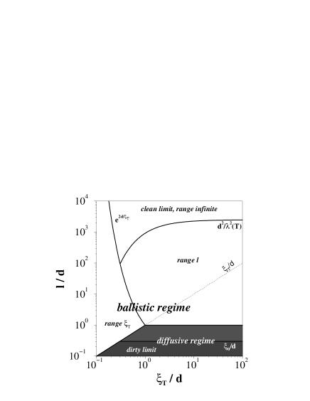
FIG. 2.: Dependence of the magnetic response on thermal length $\xi_{T}=v_{\text{F}}/2\pi T$ and mean free path $l$. In the ballistic regime $l\gg{\rm min}\{\xi_{T},d\}$ we distinguish three regions: (a) the clean limit with infinite range of the kernel exhibiting a reduced diamagnetism (overscreening), (b) the quasi-ballistic limit with finite range $\xi_{T}$ increasing screening at large temperatures, (c) the ballistic limit where the finite range $l$ enhances the screening although $l\gg d$. In the diffusive regime $l\ll\xi_{T},d$ the range of the kernel is given by $l$. The dirty limit with nearly isotropic Green’s functions is restricted to $l\ll\xi_{0},\xi_{T},d$. Note that the current-field relations can still be local or non-local depending on the relative size of penetration depth and mean free path. For comparison, the conventionally assumed border line between clean and dirty limits ($l=\xi_{T}$) is indicated by a dotted line.

A Ballistic regime

The ballistic regime is limited by $l\gg{\rm min}\{\xi_{T},d\}$, which ensures a ballistic propagation of the electrons over the thickness or the thermal length of the normal layer, respectively. As a limiting case, for $l\rightarrow\infty$ (clean limit) Eq. (9) may be solved analytically. For $T_{c}\gg T_{A}\equiv v_{\text{F}}/2\pi d$, the solution in the normal metal takes the form [6]

$$f_{0}(v_{\text{x}},x) = e^{\frac{\displaystyle 2\omega}{\displaystyle v_{\text{x}}}{\displaystyle(d-x)}}/\cosh\chi_{d}$$ (11)

$$f_{0}^{\dagger}(v_{\text{x}},x) = f(-v_{\text{x}},x),\quad\chi_{d}=\frac{2\omega d}{|v_{\text{x}}|}\;.$$ (12)

At temperatures above the Andreev temperature, $T\gg T_{A}$, only the first Matsubara frequency $\omega=\pi T$ is relevant and the decay of the $f$-function is governed by $\xi_{T}=v_{\text{F}}/2\pi T$. $T_{A}$ determines the temperature at which the $f$-function acquires a finite value at the outer boundary.

An estimation using the Eilenberger equation Eq. (9) easily shows that the clean-limit solution is valid for

$$l\gg d\exp(2d/\xi_{T})\quad \quad\xi_{T}\ll d$$ if (13)

$$l\gg d\quad \quad\xi_{T}\gg d\;.$$ if (14)

We note that this includes the region $d\ll l\ll\xi_{T}$, the finite thickness preventing the small mean free path $l\ll\xi_{T}$ of becoming effective. In the remaining part of the ballistic regime, see Fig. 2, the full solution is not known, but we may produce an approximate solution, which characterizes well the numerical results found below. Limiting ourselves to $\xi_{T}\ll d$ allows us to consider the Green’s function for the first Matsubara frequency $\omega=\pi T$ only. We restrict ourselves to the forward direction $v_{\text{x}}=+v_{\text{F}}$. From Eq. (9) we find that $f_{0}\approx 2\exp(-x/\xi_{T})$ remains unchanged as in (11), and $f_{0}^{{\dagger}}\ll 1$ and $1-g_{0}\ll 1$ obey the approximate equations,

$$\left(\frac{d}{dx}-\frac{1}{\xi_{T}}\right)f_{0}^{\dagger}(x) = -\frac{1}{l}\langle f_{0}(x)\rangle$$ (15)

$$\frac{d}{dx}(1-g_{0}(x)) = -\frac{1}{l}\langle f_{0}(x)\rangle f(x)\;$$ (16)

with the approximate solutions

$$f_{0}^{\dagger}(x) = \frac{\xi_{T}}{2l}e^{\displaystyle-x/\xi_{T}}$$ (17)

$$1-g_{0}(x) = \frac{\xi_{T}}{2l}e^{\displaystyle-2x/\xi_{T}}\;$$ (18)

Here we have used $\langle f_{0}\rangle\approx f/2$, which is valid since $f_{0}(-|v_{\text{x}}|)\ll f_{0}(|v_{\text{x}}|)$. Interestingly, while the induced superconducting correlations as described by $\langle f_{0}(x)\rangle$ remain unchanged as compared to the clean limit (11), the values of $f_{0}^{{\dagger}}$ and $1-g_{0}$ are of order $\xi_{T}/l$ rather than exponentially suppressed as in (11). This is of importance for the current response as we show below.

B Dirty limit

If impurity scattering dominates, as described by $\langle g_{0}\rangle/\tau\gg\omega$ and $\langle f_{0}\rangle/\tau\gg\Delta$, Eq. (9) can be reduced to the Usadel equation [19] for the isotropic part $\langle f_{0}(x)\rangle$. Assuming $\omega\ll\Delta$ the solution in the normal metal takes the form

$$\langle f_{0}(x)\rangle=\cosh(\sqrt{\frac{2\omega}{D}}(d-x))/\cosh(\sqrt{\frac{2\omega}{D}}d)\;,$$ (19)

where $D=v_{\text{F}}^{2}\tau/3$ is the diffusion constant. Equation (19) shows that the important energy scale is the Thouless energy $E_{\text{Th}}=D/2\pi d^{2}$. The coherence length in this case is $\xi_{D}(T)=(D/2\pi T)^{1/2}$, which reflects the diffusive nature of the electron motion.

In the normal metal $l\ll\xi_{T},d$ are necessary conditions for the Usadel theory to be valid. However, as the numerical results will confirm below, the Usadel theory in the normal metal may not be applied without considering the superconductor inducing the proximity effect. The application of the Usadel equations requires the Green’s functions to be nearly isotropic, which in the superconductor is only fulfilled for $\langle f_{0}\rangle/\tau\gg\Delta$. The validity of the Usadel theory (in the absence of fields) is thus restricted to $l\ll d,\xi_{T}$, and $l\ll\xi_{0}=v_{\text{F}}/2\pi T_{c}$, the dirty limit, see Fig. 2.

C Intermediate diffusive regime

Now we relax all restrictions on the mean free path and investigate the regime between the ballistic regime and the dirty limit. Eq. (9) can be formally decoupled using the Schopohl-Maki transformation [20]

$$a_{0}(v_{\text{x}},x)=\frac{f_{0}(v_{\text{x}},x)}{1+g_{0}(v_{\text{x}},x)},a^{\dagger}_{0}(v_{\text{x}},x)=\frac{f^{\dagger}_{0}(v_{\text{x}},x)}{1+g_{0}(v_{\text{x}},x)},$$ (20)

leading to the Riccati differential equations

$$-{v}_{x}\frac{d}{dx}a_{0}(v_{\text{x}},x)=2\tilde{\omega}(x)a_{0}(v_{\text{x}},x)+\tilde{\Delta}(x)(a^{2}_{0}(v_{\text{x}},x)-1)$$ (21)

$$v_{\text{x}}\frac{d}{dx}a^{\dagger}_{0}(v_{\text{x}},x)=2\tilde{\omega}(x)a^{\dagger}_{0}(v_{\text{x}},x)+\tilde{\Delta}(x)(a^{\dagger 2}_{0}(v_{\text{x}},x)-1).$$ (22)

Eqs. (22) provide the basis for a (stable) numerical solution. We have determined the impurity self-energies self-consistently by an iteration procedure starting from the dirty-limit expression. Representative results of the numerical calculation are shown in Fig. 3.

FIG. 3.: Spatial dependence of the anomalous Green’s function $f_{0}(x,v_{x})$ in a proximity normal-metal layer. The thickness is $d=10v_{\text{F}}/T_{c}$ and the frequency is $\omega=v_{F}/d$. The mean free path is $l=d$ in (a) and $l=0.1d$ in (b). The insets show the angular dependence $f(v_{\text{Fx}})$ at the positions indicated by the arrows. We note that in the Usadel theory the angular dependence would be given by a linear function.

We have chosen the frequency $\omega=v_{F}/d$ and a mean free path of $l=d$ in Fig. 3(a), $l=0.1d$ in Fig. 3(b). Note the distinction of the $f$-function for forward ($v_{\text{Fx}}=v_{\text{F}}$, solid line) and backward propagation ($v_{\text{Fx}}=-v_{\text{F}}$, dashed line). As we cross over from the ballistic to the diffusive regime, the backward propagating branch changes from a monotonically increasing $f$-function of $x$ for $l=d$ to a decaying $f$-function for $l=0.1d$. In the ballistic case the backward moving electrons carry superconducting correlations only after reflection from the normal-metal–vacuum boundary $x=d$. In the diffusive case, the backward propagating $f$-function is generated by the impurity scattering from the forward branch, thus taking the same functional dependence of $x$, see Fig. 3. This behavior is illustrated in the insets, where $f$ is plotted as a function of $v_{\text{x}}$ for fixed positions. The sharp features present in Fig. 3(a) are washed out by impurity scattering in 3(b). Remarkably, however, they are still far from the dirty-limit behavior, for which $f_{0}(v_{\text{Fx}})$ in the insets is expected to be a straight line. According to conventional wisdom $\l=0.1v_{\text{F}}/\omega\ll\xi_{T}$ would indicate the dirty limit. Considering that we have chosen $d=10v_{\text{F}}/T_{c}$, implying $l\approx v_{\text{F}}/\Delta$, we notice that the dirty-limit condition is not fulfilled in the superconductor. The anisotropy of the $f$-function present in the superconductor by proximity induces an anisotropy inside the normal metal, which is not accurately described by the Usadel theory. For the dirty-limit theory to be valid in the normal metal, the superconductor has to be dirty as well.

We note that in our present calculation we have assumed the same mean free path in the superconductor and the normal metal. Allowing for different mean free paths would affect the definition of the dirty and the intermediate regime, and we do not further investigate this question here.

III Linear-response kernel

In this section we derive the general linear-response kernel (44) of a normal-metal–superconductor sandwich in terms of the Green’s functions in absence of the fields. We consider the quasi-one-dimensional system shown in Fig. 1, assuming a superconductor of thickness $d_{s}$ and a normal metal of thickness $d$. The magnetic field is applied in $z$-direction as described by the gauge $\mathchoice{{\hbox{\boldmath$\displaystyle A$}}}{{\hbox{\boldmath$\textstyle A$}}}{{\hbox{\boldmath$\scriptstyle A$}}}{{\hbox{\boldmath$\scriptscriptstyle A$}}}=A(x)\mathchoice{{\hbox{\boldmath$\displaystyle e$}}}{{\hbox{\boldmath$\textstyle e$}}}{{\hbox{\boldmath$\scriptstyle e$}}}{{\hbox{\boldmath$\scriptscriptstyle e$}}}_{y}$. To calculate the linear diamagnetic response, we separate the Green’s functions into its real and imaginary parts, where the imaginary part is of first order in $A$ and the real part of zeroth order:

$$f(\mathchoice{{\hbox{\boldmath$\displaystyle v$}}}{{\hbox{\boldmath$\textstyle v$}}}{{\hbox{\boldmath$\scriptstyle v$}}}{{\hbox{\boldmath$\scriptscriptstyle v$}}}_{\text{F}},\mathchoice{{\hbox{\boldmath$\displaystyle x$}}}{{\hbox{\boldmath$\textstyle x$}}}{{\hbox{\boldmath$\scriptstyle x$}}}{{\hbox{\boldmath$\scriptscriptstyle x$}}}) = f_{0}(v_{\text{x}},x)+if_{1}(v_{\text{x}},v_{\text{y}},x)$$ (23)

$$f^{\dagger}(\mathchoice{{\hbox{\boldmath$\displaystyle v$}}}{{\hbox{\boldmath$\textstyle v$}}}{{\hbox{\boldmath$\scriptstyle v$}}}{{\hbox{\boldmath$\scriptscriptstyle v$}}}_{\text{F}},\mathchoice{{\hbox{\boldmath$\displaystyle x$}}}{{\hbox{\boldmath$\textstyle x$}}}{{\hbox{\boldmath$\scriptstyle x$}}}{{\hbox{\boldmath$\scriptscriptstyle x$}}}) = f^{\dagger}_{0}(v_{\text{x}},x)+if^{\dagger}_{1}(v_{\text{x}},v_{\text{y}},x)$$ (24)

$$g(\mathchoice{{\hbox{\boldmath$\displaystyle v$}}}{{\hbox{\boldmath$\textstyle v$}}}{{\hbox{\boldmath$\scriptstyle v$}}}{{\hbox{\boldmath$\scriptscriptstyle v$}}}_{\text{F}},\mathchoice{{\hbox{\boldmath$\displaystyle x$}}}{{\hbox{\boldmath$\textstyle x$}}}{{\hbox{\boldmath$\scriptstyle x$}}}{{\hbox{\boldmath$\scriptscriptstyle x$}}}) = g_{0}(v_{\text{x}},x)+ig_{1}(v_{\text{x}},v_{\text{y}},x)\;.$$ (25)

The zeroth-order parts obey Eq. (9) discussed in the previous section. The first-order parts of Eq. (2) read

$$-{v}_{x}\frac{d}{dx}f_{1}(v_{\text{x}},v_{\text{y}},x)=2\tilde{\omega}(x)f_{1}(v_{\text{x}},v_{\text{y}},x)$$ (27)

$$-2\tilde{\Delta}(x)g_{1}(v_{\text{x}},v_{\text{y}},x)+2ev_{\text{y}}A(x)f_{0}(v_{\text{x}},x)$$

$${v}_{x}\frac{d}{dx}f^{\dagger}_{1}(v_{\text{x}},v_{\text{y}},x)=2\tilde{\omega}(x)f^{\dagger}_{1}(v_{\text{x}},v_{\text{y}},x)$$ (29)

$$-2\tilde{\Delta}(x)g_{1}(v_{\text{x}},v_{\text{y}},x)+2ev_{\text{y}}A(x)f^{\dagger}_{0}(v_{\text{x}},x)\;.$$

where $\tilde{\omega}(x)$, $\tilde{\Delta}(x)$ were given after Eq. (9) and

$$g_{1}(v_{\text{x}},v_{\text{y}},x)=$$ (31)

$$-\frac{f_{0}(v_{\text{x}},x)f^{\dagger}_{1}(v_{\text{x}},v_{\text{y}},x)+f_{1}(v_{\text{x}},v_{\text{y}},x)f^{\dagger}_{0}(v_{\text{x}},x)}{2g_{0}(v_{\text{x}},x)}$$

follows from the normalization (7). We now apply the Maki-Schopohl transformation defined in (20) to the full equations of motions (2). After linearization we obtain

$$f_{1}(v_{\text{x}},v_{\text{y}},x) = 2\frac{a_{1}(v_{\text{x}},v_{\text{y}},x)-a_{0}^{2}(v_{\text{x}},x)a^{\dagger}_{1}(v_{\text{x}},v_{\text{y}},x)}{(1+a_{0}(v_{\text{x}},x)a^{\dagger}_{0}(v_{\text{x}},x))^{2}}$$

$$f^{\dagger}_{1}(v_{\text{x}},v_{\text{y}},x) = 2\frac{a^{\dagger}_{1}(v_{\text{x}},v_{\text{y}},x)-a^{\dagger 2}_{0}(v_{\text{x}},x)a_{1}(v_{\text{x}},v_{\text{y}},x)}{(1+a_{0}(v_{\text{x}},x)a^{\dagger}_{0}(v_{\text{x}},x))^{2}}\;,$$

and Eqs. (27) are decoupled into

$$-\frac{v_{\text{x}}}{2}\frac{d}{dx}a_{1}(v_{\text{x}},v_{\text{y}},x)=$$ (32)

$$\left[\tilde{\omega}(x)+\tilde{\Delta}(x)a_{0}(v_{\text{x}},x)\right]a_{1}(v_{\text{x}},v_{\text{y}},x)+ev_{\text{y}}A(x)a_{0}(v_{\text{x}},x)$$ (33)

$$\frac{v_{\text{x}}}{2}\frac{d}{dx}a^{\dagger}_{1}(v_{\text{x}},v_{\text{y}},x)=$$ (34)

$$\left[\tilde{\omega}(x)+\tilde{\Delta}(x)a^{\dagger}_{0}(v_{\text{x}},x)\right]a^{\dagger}_{1}(v_{\text{x}},v_{\text{y}},x)+ev_{\text{y}}A(x)a^{\dagger}_{0}(v_{\text{x}},x).$$ (35)

For a more general form of these equations that has been used to treat the linear electromagnetic response of vortices numerically, see [21]. We will now proceed analytically. As a consequence of Eq. (32) we find $a_{1}(-v_{\text{y}})=-a_{1}(v_{\text{y}})$ and the same for $a^{\dagger}_{1}$, which leads to $\langle f_{1}\rangle=\langle f^{\dagger}_{1}\rangle=0$, as was already noted above. Furthermore, since $a^{\dagger}_{1}(v_{\text{x}})=a_{1}(-v_{\text{x}})$, we only have to consider one of the two equations (e.g., the first one). Equation (32) is an inhomogeneous first-order differential equation, which can be integrated analytically. Assuming that $f$ and $f^{{\dagger}}$ do not change sign with the help of (9) the solution can be written as

$$a_{1}(v_{\text{x}},v_{\text{y}},x)=c(v_{\text{x}},v_{\text{y}})\frac{m(v_{\text{x}},x,x_{0})}{f^{\dagger}_{0}(v_{\text{x}},x)}$$ (37)

$$-\frac{2ev_{\text{y}}}{v_{\text{x}}f^{\dagger}_{0}(v_{\text{x}},x)}\int_{x_{0}}^{x}[1-g_{0}(v_{\text{x}},x^{\prime})]m(v_{\text{x}},x,x^{\prime})A(x^{\prime})dx^{\prime}$$

where

$$m(v_{\text{x}},x,x^{\prime})=\exp\left(\frac{2}{v_{\text{x}}}\int_{x}^{x^{\prime}}\frac{\tilde{\Delta}(x^{\prime\prime})}{f^{\dagger}_{0}(v_{\text{x}},x^{\prime\prime})}dx^{\prime\prime}\right)$$ (38)

In this equation $x_{0}$ is an arbitrary reference point and the constant $c$ has to be determined by the appropriate boundary conditions. $m$ satisfies the relations of a propagator, $m(u,x,x^{\prime})=m(u,x^{\prime},x)^{-1}$ and $m(u,x,x^{\prime\prime})m(u,x^{\prime\prime},x^{\prime})=m(u,x,x^{\prime})$. Now we determine the constant $c$ for a system of size $[-d_{s},d]$. We assume specular reflection at two boundaries at $x=-d_{s},d$ and ideal interfaces between different materials inside the system. The appropriate boundary conditions are $f(v_{\text{x}},v_{\text{y}},x=-d_{s},d)=f(-v_{\text{x}},v_{\text{y}},x=-d_{s},d)$ and continuity at the internal interfaces. The same conditions are valid for $a_{1}$ and $a^{\dagger}_{1}$. This leads to

$$c(v_{\text{x}},v_{\text{y}}) = 2e\frac{v_{\text{y}}}{v_{\text{x}}}\int_{-d_{s}}^{d}\frac{m(v_{\text{x}},d,x^{\prime})+m(-v_{\text{x}},d,x^{\prime})}{m(v_{\text{x}},d,-d_{s})-m(-v_{\text{x}},d,-d_{s})}$$ (40)

$$\times[1-g_{0}(v_{\text{x}},x^{\prime})]A(x^{\prime})dx^{\prime}\;\hfill.$$

The current is determined by Eq. (8), using the Green’s functions (31), expressed by the solution (37). We obtain the following general result for the linear current response in functional dependence of the vector potential,

$$j_{y}(x)=-\int\limits_{-d_{s}}^{d}K(x,x^{\prime})A(x^{\prime})dx^{\prime}\;,$$ (41)

where the kernel $K(x,x^{\prime})$ is given by

$$K(x,x^{\prime}) = \frac{e^{2}p_{F}^{2}}{\pi}T\sum_{\omega>0}\int\limits_{0}^{v_{F}}\text{d}u\,\frac{v_{F}^{2}-u^{2}}{{v_{F}^{2}}u}[1+g_{0}(u,x)][1-g_{0}(u,x^{\prime})]\bigg{[}\Theta(x-x^{\prime})m(u,x,x^{\prime})+\Theta(x^{\prime}-x)m(-u,x,x^{\prime})$$ (44)

$$+\frac{m(-u,x,d)m(u,d,x^{\prime})}{1-m(u,d,-d_{s})m(-u,-d_{s},d)}+\frac{m(u,x,-d_{s})m(-u,-d_{s},x^{\prime})}{1-m(u,d,-d_{s})m(-u,-d_{s},d)}$$

$$+\frac{m(-u,x,d)m(u,d,-d_{s})m(-u,-d_{s},x^{\prime})}{1-m(u,d,-d_{s})m(-u,-d_{s},d)}+\frac{m(u,x,-d_{s})m(-u,-d_{s},d)m(u,d,x^{\prime})}{1-m(u,d,-d_{s})m(-u,-d_{s},d)}\bigg{]}\;.$$

Equation (44) gives the exact linear-response kernel of any quasi-one-dimensional system, consisting of a combination of normal and superconducting layers extending from $x=-d_{s}$ to $x=d$. The kernel is expressed in terms of the quasi-classical Green’s functions in absence of the fields, which may be specified for the particular problem of interest. We note two characteristic features of Eq. (44): The factor $(1-g_{0}(u,x^{\prime}))$ measures the deviation of a quasi-classical trajectory from the normal state $g_{0}\equiv 1$, which is inert to a magnetic field. The propagator $m(u,x,x^{\prime})$ shows up in six summands which represent all the ballistic paths from $x$ to $x^{\prime}$, accounting for multiple reflection at the walls at $-d_{s}$ and $d$. Thus the first two summands connecting $x$ and $x^{\prime}$ directly constitute the bulk contribution, while the additional four summands are specific to a finite system (assuming specular reflection at the boundary). We note that a form similar to (44) may be derived for non-ideal interfaces between the normal and superconducting layers, if the appropriate boundary conditions following from Ref. [22] are taken into account (these boundary conditions are only valid if the distance between two barriers is larger than the mean free path).

For illustration we reproduce the current response of a half-infinite superconductor. Setting $d=0$ and $d_{s}\to\infty$, the solution of the Eilenberger equation (9) takes the simple form $g_{0}=\omega/\Omega$, $f_{0}=f^{{\dagger}}_{0}=\Delta/\Omega$, where $\Omega=(\Delta^{2}+\omega^{2})^{1/2}$. Inserting in (44) we obtain the linear-response kernel

$$K_{S}(x,x^{\prime}) = \frac{e^{2}p_{F}^{2}}{\pi}T\sum_{\omega>0}\frac{\Delta^{\!2}}{\Omega^{2}}\int\limits_{0}^{v_{F}}\!\!du\frac{1\!-\!u^{2}/v_{F}^{2}}{u}$$ (46)

$$\times\big{[}e^{-(2\Omega+\frac{\scriptstyle 1}{\scriptstyle\tau})\frac{\scriptstyle|x-x^{\prime}|}{\scriptstyle u}}\!\!+e^{(2\Omega+\frac{\scriptstyle 1}{\scriptstyle\tau})\frac{\scriptstyle x+x^{\prime}}{\scriptstyle u}}\big{]}\;,$$

which describes the current response of an arbitrary superconductor, as first derived by Gorkov[23], which here additionally includes the effect of the boundary. For fields varying rapidly spatially we arrive at a non-local current-field relation of the Pippard-type[14], while for slowly varying fields the kernel can be integrated out in Eq. (41), producing the London result[13]. We recall here certain generic features of this kernel, which are of importance below. In a dirty superconductor ($\Omega\ll 1/\tau$) the range is given by the mean free path $l=v_{F}\tau$. In a clean superconductor ($1/\tau\ll\Omega$), the range is roughly given by the coherence length $\xi_{0}$ and is thus nearly temperature-independent.

IV Magnetic response

For the NS system we consider in this paper, see Fig. 1, the kernel (44) may be simplified using $m(u,x,-\infty)\rightarrow 0$ and $m(-u,-\infty,x)\rightarrow 0$ as $d_{s}\to\infty$ ($u>0$). The linear-response kernel takes the form,

$$K(x,x^{\prime}) = -\frac{e^{2}p_{F}^{2}}{\pi}T\sum_{\omega>0}\int\limits_{0}^{v_{F}}du\frac{v_{F}^{2}-u^{2}}{v_{F}^{2}u}(1+g_{0}(u,x))(1-g_{0}(u,x^{\prime}))$$ (48)

$$\bigg{[}\Theta(x-x^{\prime})m(u,x,x^{\prime})+\Theta(x^{\prime}-x)m(-u,x,x^{\prime})+m(-u,x,d)m(u,d,x^{\prime})\bigg{]}\;.$$

The magnetic response of the proximity system follows from the self-consistent solution of Eq. (41) and the Maxwell equation

$$\frac{d^{2}}{dx^{2}}A(x)=-4\pi j_{y}(x)\;.$$ (49)

As boundary condition we use $\frac{d}{dx}A(x)|_{x=d}=H$, where $H$ is the applied magnetic field, and $A(0)=0$, neglecting the penetration of the field into the superconductor. The inclusion of the field penetration into the superconductor leads to corrections $\sim\lambda_{\text{S}}/d$ to $\rho$, which is a small ratio for typical proximity systems. Here $\lambda_{\text{S}}$ is the effective penetration depth of the superconductor, including the nonlocal or impurity effects. The magnetic response of the normal-metal layer is measured by the screening fraction $\rho=-4\pi\chi=1-A(d)/Hd$, which gives the fraction of the normal-metal layer that is effectively field free. It is given by the susceptibility $\chi$, which is equal to the ratio of the average magnetization to the applied magnetic field.

The general properties of the kernel (44) are characterized by both the decay (range) of the propagator $m(v_{F},x,x^{\prime})$ and the amplitude of the prefactor $(1+g_{0})(1-g_{0})$ which determines the degree of non-locality of the relations (41). The inverse decay length of the propagator is proportional to the off-diagonal part of the self-energy $\tilde{\Delta}$ and the prefactor is related to the superfluid density. We discuss below how, in the proximity effect, the range of the kernel varies from infinity to $l$ and $\xi_{T}$, exhibiting a strong temperature dependence, which leads to non-trivial screening properties. Furthermore, the superfluid density introduces an additional length scale in the problem: the London length $\lambda_{N}$, which becomes crucial for the distinction of various regimes.

A Clean limit

A special case is the clean normal metal ($l\to\infty$). Here the range is infinite and the current-field relation is completely non-local. It follows from (44) that it is necessary to have impurities in a normal metal to get a finite range of the kernel. In the limit $d\gg\xi_{0}$ the current may be written as

$$j_{\text{clean}}=-\frac{1}{4\pi\lambda^{2}(T)\,d}\int\limits_{0}^{d}A(x)dx\;.$$ (50)

This defines a temperature-dependent penetration depth that can be given explicitly in the limits $T=0$ and $T\gg T_{A}$:

$$\lambda^{2}(T)=\left\{\begin{array}[c]{ll}\displaystyle\frac{m}{4\pi e^{2}n_{e}}=:\lambda_{N}^{2}&;\;T=0\\[14.22636pt] \displaystyle\frac{\lambda_{N}^{2}T}{12T_{A}}e^{2\frac{T}{T_{A}}}&;\;T\gg T_{\text{A}}.\end{array}\right.$$ (51)

Solving Maxwell’s equation we find

$$A(x)=Hx(1-\frac{3}{4}\frac{d(2d-x)}{(3\lambda^{2}(T)+d^{2})}),$$ (52)

and the screening fraction

$$\rho=\frac{3}{4+12\lambda^{2}(T)/d^{2}}\;.$$ (53)

In the limit $\lambda(T)\ll d$ the screening fraction is $3/4$, thus the screening is not perfectly diamagnetic. The magnetic field inside the normal metal is $B(x)/H=1-2\rho(1-x/d)$, showing the effect of overscreening for $\rho>1/2$, where the field reverses sign inside the normal metal.

B Dirty limit

Using the fact that the zeroth-order Green’s function is nearly isotropic and varies on a scale $\xi_{D}(T)\gg l$, we find for the kernel (48)

$$K(x,x^{\prime}) = -\frac{e^{2}p_{F}^{2}}{\pi}T\sum_{\omega>0}\langle f(x)\rangle^{2}\int\limits_{0}^{v_{F}}du\frac{v_{F}^{2}-u^{2}}{v_{F}^{2}u}$$ (55)

$$\times\left[e^{-\frac{|x-x^{\prime}|}{lu}}+e^{\frac{2d-x-x^{\prime}}{lu}}\right]\;.$$

The kernel is factorized in a part containing the temperature dependence and a part which is responsible for the non-locality. The current is then expressed as

$$j(x)=-\frac{1}{4\pi\lambda^{2}(x,T)}\int\limits_{0}^{d}K_{d}(x,x^{\prime})A(x^{\prime})dx^{\prime}\;.$$ (56)

The local penetration depth $\lambda(x,T)$ is defined as

$$\frac{1}{\lambda^{2}(x,T)}=\frac{4\pi\tau}{\lambda_{N}^{2}}T\sum_{\omega>0}\langle f(x)\rangle^{2}$$ (57)

and the temperature-independent part of the kernel is given by

$$K_{d}(x,x^{\prime}) = \frac{3}{4l}\left[E_{1}(\frac{|x-x^{\prime}|}{l})-E_{3}(\frac{|x-x^{\prime}|}{l})\right.$$ (59)

$$\left.+E_{1}(\frac{2d-x-x^{\prime}}{l})-E_{3}(\frac{2d-x-x^{\prime}}{l})\right]\;.$$

In this formula $E_{n}(z)=\int_{1}^{\infty}t^{-n}\exp(-zt)dt$ is the exponential integral. For $\lambda(x,T)\gg l$ the vector potential may be taken out of the integral in Eq. (56) and the spatial integral yields the well-known local current-vector potential relation used in Usadel theory[19]. We note that for $\lambda\ll\xi_{0}$ there may exist a region (see Fig. 2) where the Green’s functions are nearly isotropic, and in absence of the field are given by Usadel theory, but the current response is nonlocal. To put limits on the validity of the local relation, we consider the approximate form $\langle f\rangle\sim\exp[-x(2\omega/D)^{1/2}]$ to determine the local penetration depth. As a result we find

$$\lambda(x,T)\approx\left\{\begin{array}[c]{ll}\lambda_{N}\frac{x}{l}&\text{if}\quad\xi_{D}(T)\gg d\\ \lambda_{N}\frac{\xi_{D}(T)}{l}e^{x/\xi_{D}(T)}&\text{if}\quad\xi_{D}(T)\ll d\;.\end{array}\right.$$ (60)

To achieve locality we need to have $l<\lambda(x,T)$ in the region, where the screening takes place. For $T\ll D/d^{2}$ this means $l\ll\lambda(d)$ leading to the condition $l^{2}\ll\lambda_{N}d$. For $T\gg D/d^{2}$ screening takes place at $x\approx\xi_{D}$ and we have $l^{2}\ll\lambda_{N}\xi_{D}(T)$. The local penetration depth at the outer boundary can be small compared to $d$. In that case the screening fraction $\rho=1-\lambda(d)/d$ can reach practically unity.

At high temperatures $T\gg E_{\text{Th}}$, the inverse penetration depth is exponentially suppressed on a scale of the temperature-dependent coherence length $\xi_{D}(T)$. This length defines the screening region and consequently

$$\rho(T)\propto\frac{\xi_{D}(T)}{d}\propto T^{-1/2}\;.$$ (61)

This result has already been obtained on the basis of Ginzburg-Landau theory [5] and numerically confirmed using Usadel theory [24]. We expect that non-local screening, which may be taken into account using Eq. (59), will only lead to quantitative corrections to Eq. (61). We will not consider this here but concentrate on the more interesting case in which non-locality gives rise to a qualitatively different picture.

C Arbitrary impurity concentration: numerical results

As has been shown in the last two subsections, there are two main differences in the observable properties of the induced screening in the clean or the dirty limit. Firstly, the saturation value of $\rho$ in the dirty limit can reach practically unity, whereas in the clean limit it is limited to $3/4$. The analytic behavior at high temperatures is quite different too. In the dirty limit $\rho$ shows an algebraic behavior $\propto T^{-1/2}$, whereas in the clean limit we find $\rho\propto\exp(-2T/T_{A})$. From a theoretical point of view these two limits are characterized by a completely nonlocal constitutive relation in the clean limit and a local relation in the dirty limit. In this section we will investigate the magnetic response in the regime between these two extreme cases.

To calculate the diamagnetic response, we have evaluated the integral kernel in Eq. (48) numerically using the results from the Sec. II and solving Maxwell’s equation by a finite-difference technique. Therefore, the parameters entering the calculation are $l/d$ and $\lambda_{N}/d$, assuming $l>\xi_{0}$, and $\xi_{T}/d$ giving the temperature dependence.

Magnetic field distributions for various impurity concentrations and temperatures are shown in Fig. 4. Thick lines show the magnetic field and thin lines the current distribution inside the normal metal. Different graphs correspond to different mean free paths and the curves inside each graph to different temperatures. In all curves we have chosen $\lambda_{N}=0.003d$. All these curves clearly show deviations from the clean-limit behavior, where the field decays linearly and the current density is spatially constant. Larger impurity concentrations make it possible to localize the current on a length scale smaller than system size. Obviously, this scale is not given by the mean free path, but can be considerably smaller. Later we will show what determines this length scale. Whether the localization of the current increases or decreases the screening fraction depends on temperature. Note that for all parameters chosen the field is overscreened, which is the signature of a nonlocal constitutive relation.

FIG. 4.: Magnetic induction (thick lines) and current densities (thin lines) in a proximity layer for different mean free paths. The different curves in each graph correspond to temperatures of $T/T_{A}=0.04$ (solid line), $5$ (short-dashed line), and $8$ (long-dashed line).

FIG. 5.: Numerical results for screening fraction of the normal metal layer for $\lambda_{N}=0.003d$. The clean limit is indicated by a thin line reaching $\rho=0.75$ for $T\to 0$. Even a very large mean free path of $10^{4}d$ leads to an enhanced screening at low temperatures. For smaller mean free paths (but still $>d$) the screening is enhanced at high and low temperatures. At the smallest mean free path $0.1d$ the system is in the diffusive regime leading to a completely different temperature dependence.

The screening fraction as a function of temperature is shown in Fig. 5. The different curves are for the clean limit and for mean free paths $l/d=10^{4},10,1,0.1$. We see that a finite impurity concentration has strong influence on the screening fraction, even if $l>d$. It can either increase or decrease the diamagnetic screening, depending on temperature.

For the interpretation of these results we first consider the case $l=0.1d$. The lower-right graph in Fig. 4 shows that the screening is nearly local, since overscreening is rather small. The local screening strength depends on the local superfluid density. At low temperatures $T\ll T_{A}$ the superfluid density at $x=d$ is finite and the field is screened exponentially, leading to a screening fraction of nearly unity. A higher temperature suppresses the superfluid density and the field penetrates to the point where the density is large enough to screen effectively. On the other hand, the locality of the kernel allows the system to screen even if the superfluid density is suppressed nearly everywhere. The screening is then enhanced in comparison to the clean limit. In Fig. 5 this appears at $T\approx 6T_{A}$.

Let us now consider a mean free path of order or much larger than the sample size. Even for $l=10^{4}d$ we see a deviation from the clean-limit expression at low temperatures. For $l=10d$ and $l=d$ screening is enhanced in comparison to the clean limit at low and high temperatures. Only in an intermediate regime, i. e. around $T=5T_{A}$ in our case, $\rho$ is similar to the clean limit screening fraction. A qualitative understanding may be gained from looking at the constitutive relation in the limit $l\gg d$. In the limit $T\ll T_{A}$ the zeroth-order Green’s functions are given by the clean-limit expressions (11). We approximate the kernel (48) by

$$K(x,x^{\prime})=\frac{1}{8\pi\lambda^{2}(T)d}\left[e^{-\frac{|x-x^{\prime}|}{l}}+e^{-\frac{2d-x-x^{\prime}}{l}}\right]\;.$$ (62)

Since $l\gg d$, the exponentials may be expanded to first order. As a result, we obtain two contributions to the current

$$j_{\text{clean}} = \frac{-1}{4\pi\lambda^{2}(T)d}\int_{0}^{d}A(x)dx$$ (63)

$$j_{\text{imp}}(x) = \frac{1}{8\pi\lambda^{2}(T)d}\int_{0}^{d}\frac{|x-x^{\prime}|+2d-x-x^{\prime}}{l}A(x^{\prime})dx^{\prime}\;.$$ (65)

When will deviations from the clean limit become important? It is clear that the impurities cannot be neglected, if (LABEL:jyimp) is comparable to (63). We estimate this by calculating the two contributions to the current using the clean-limit vector potential (52). Comparing the two contributions, we find that impurities can be neglected, if

$$\lambda_{\text{eff}}(T)\equiv\sqrt[3]{\lambda^{2}(T)l}\gg d\;.$$ (66)

This equation defines a new length scale, the effective penetration depth $\lambda_{\text{eff}}$, which determines the validity of the clean-limit magnetic response. For the clean limit to be valid at $T=0$ the condition $\lambda_{\text{eff}}(0)>d$ has to be fulfilled, since in this case the screening takes place on the geometrical scale $d$. In the case $\lambda_{\text{eff}}(0)\ll d$ the field is screened on a scale $\lambda_{\text{eff}}$ and the screening fraction is strongly enhanced in comparison to the clean limit. Nevertheless, the clean-limit behavior reappears at higher temperatures, since $\lambda_{\text{eff}}(T)$ grows with temperature.

For $T\gg T_{A}$ the deviations from the clean limit are related to deviations of the zeroth-order Green’s function from the clean-limit expression due to impurity scattering. The correction to $g$, given in Eq. (18), leads to a finite superfluid density in the vicinity of the superconductor via the factor $1-g(x^{\prime})$ in the kernel. The range of the propagator is modified by the correction (17) to $f^{\dagger}$, leading to

$$m(x,x^{\prime})=\exp\left(\frac{1}{l}\int_{x}^{x^{\prime}}dx^{\prime\prime}\frac{\langle f(x^{\prime\prime})\rangle}{f^{\dagger}(x^{\prime\prime})}\right)\approx\exp\left(2\frac{x^{\prime}-x}{\xi_{T}}\right)\;.$$ (67)

Thus, the range of the kernel is now given by $\xi_{T}$, which is strongly temperature dependent. Summarizing, we find for the current

$$j(x)\approx\frac{-1}{\lambda_{\text{eff}}(0)^{3}}\int_{0}^{d}dx^{\prime}e^{-2\frac{x^{\prime}+|x-x^{\prime}|}{\xi_{T}}}A(x^{\prime})\;,$$ (68)

again showing the importance of the new length scale $\lambda_{\text{eff}}$. In the limit $\lambda_{\text{eff}}(0)\gg\xi_{T}$ the field cannot be effectively screened on the scale $\xi_{T}$, leading to a vanishing screening fraction. If $\lambda_{\text{eff}}(0)\ll\xi_{T}$ the field can be screened on a length scale smaller than $\xi_{T}$ and the screening fraction will be finite.

It is therefore evident that the interplay between local and nonlocal physics is of crucial importance for the screening behavior of a normal-metal proximity layer. The most interesting regime occurs for $l>d$, where a transition between different screening behaviors may be observed by varying the temperature, see Fig. 2.

We note that the screening fraction is a non-monotonic function of the mean free path. At low temperature, with increasing mean free path (i.e. increasing purity), the screening fraction is reduced rather than enhanced. Assuming a temperature-dependent scattering mechanism with decreasing mean free path as a function of temperature, such as electron-electron or electron-phonon interaction, we might speculate to observe a non-monotonic (i.e. re-entrant) behavior of the susceptibility (here the smallness of the scattering rate is compensated by the high sensibility of the non-local current-field relation). However, as is evident from Eq. (38), the largest off-diagonal self-energy ($\tilde{\Delta}$) which includes e.g. impurity scattering will provide a (low-temperature) cutoff for this behavior.

Finally we comment on the effect of a rough boundary. For $T\gg T_{A}$ the Green’s functions are independent of the boundary condition at $x=d$. In this case a finite screening fraction can only be due to impurity scattering, see Fig. 5. For $T<T_{A}$ the screening behavior will be strongly affected by a rough boundary. This makes it possible to distinguish between clean samples with a rough boundary and samples containing impurities.

V Conclusions

We have investigated the diamagnetic response of a proximity layer for arbitrary impurity concentration using the quasiclassical theory of superconductivity. We found a variety of different regimes in which the physics is different from the previously studied clean and dirty limits.

We have first investigated the proximity effect in the absence of fields, distinguishing three different regimes, see Fig. 2. In the ballistic regime, the validity of the clean-limit solution is restricted to $l\gg d\exp(2d/\xi_{T})$ for $\xi_{T}\ll d$ and to $l\gg d$ for $\xi_{T}\gg d$. The last condition is the consequence of the suppression of the density of states for $\omega\ll v_{\text{F}}/d$, which enhances the effective mean free path to $\sim lv_{\text{F}}/\omega d$. In the diffusive regime, we found that the validity of the Usadel equation (dirty limit) depends on the superconductor as well as the normal metal, and is thus restricted to $l\ll\xi_{0}$ and $l\ll d,\xi_{T}$. The first condition is due to the fact that the induced superconducting correlations are strongly anisotropic for a clean superconductor ($l\gg\xi_{0}$), even if the motion is diffusive in the normal metal. The intermediate diffusive regime ($\xi_{0}\ll l\ll d$) is not covered by these two cases. Here the full Eilenberger equation has to be solved, which requires a numerical analysis, see Fig. 3.

To study the magnetic response of the proximity layer we have derived explicit expressions for the general linear-response kernel (44) for an NS sandwich. This derivation may easily be generalized to systems such as Josephson junctions or unconventional superconductors. We have used this linear-response kernel to study the magnetic response of the proximity system at arbitrary impurity concentrations. The nonlocal current-field relation is shown to have non-trivial consequences on the screening behavior of the normal metal. In the ballistic case, we found the clean-limit theory to be restricted further by $d<(\lambda^{2}(T)l)^{1/3}=\lambda_{\text{eff}}$, $\lambda_{\text{eff}}$ giving the penetration depth for the non-local current-field relation. If $\lambda_{\text{eff}}>d$, the screening takes place on the geometric length scale $d$, leading to a saturation at the screening fraction of $3/4$ at low temperatures. If $\lambda_{\text{eff}}<d$, the finite (even though large) mean free path strongly enhances the screening. Thus for typical samples with $\lambda_{N}\ll d$ even a mean free path $l\gg d$ cannot be neglected, i.e., the clean-limit behavior is practically unobservable. At large temperatures $T\gg T_{A}$, a finite impurity concentration reduces the range of the linear-response kernel to $\xi_{T}$, again enhancing the screening. Furthermore, the screening fraction may serve to distinguish between samples with bulk impurities rather than a rough boundary, since a nonzero screening fraction at large temperatures is only due to bulk impurity scattering. In dirty systems, where the zeroth-order Green’s function is well described by the Usadel approximation, the current-field relation can still be non-local. We have shown that the applicability of the local current-field relation is restricted to $l^{2}\ll\lambda_{N}d$ for $T\ll E_{\text{Th}}$ and $l^{3}\ll\lambda_{N}^{2}\xi_{D}(T)$ for $T\gg E_{\text{Th}}$. This shows that in the presence of magnetic fields some caution is needed in applying the Usadel theory.

We would like to acknowledge discussions with G. Blatter, G. Schön, F. K. Wilhelm, and A. D. Zaikin. A. L. F. is grateful to Universität Karlsruhe for hospitality, C. B. and W. B. would like to thank ETH Zürich for hospitality and were supported by the Deutsche Forschungsgemeinschaft (grant No. Br1424/2-1) and the German Israeli Foundation (Contract G-464-247.07/95).

REFERENCES

- [1] A. C. Mota, D. Marek, and J. C. Weber, Helv. Phys. Acta 55, 647 (1982).
- [2] Th. Bergmann, K. H. Kuhl, B. Schröder, M. Jutzler, and F. Pobell, J. Low Temp. Phys. 66, 209 (1987).
- [3] P. Visani, A. C. Mota, and A. Pollini, Phys. Rev. Lett. 65, 1514 (1990).
- [4] A. C. Mota, P. Visani, A. Pollini, and K. Aupke, Physica B 197, 95 (1994).
- [5] Orsay Group on Superconductivity, in Quantum Fluids, ed. D. Brewer (North-Holland, Amsterdam, 1966).
- [6] A. D. Zaikin, Solid State Commun. 41, 533 (1982).
- [7] S. Higashitani and K. Nagai, J. Phys. Soc. Jpn. 64, 549 (1995).
- [8] W. Belzig, C. Bruder, and G. Schön, Phys. Rev. B 53, 5727 (1996).
- [9] A. L. Fauchère and G. Blatter, Phys. Rev. B 56, 14102 (1997).
- [10] Y. Oda and H. Nagano, Solid State Commun. 35, 631 (1980).
- [11] A. C. Mota, P. Visani, and A. Pollini, J. Low Temp. Phys. 76, 465 (1989).
- [12] H. Onoe, A. Sumuiyama, M. Nakagawa, and Y. Oda, J. Phys. Soc. Jpn. 64, 2138 (1995).
- [13] F. and H. London, Proc. Phys. Soc., A149, 71 (1938).
- [14] A. B. Pippard, Proc. Roy. Soc. 216, 547 (1953).
- [15] G. Eilenberger, Z. Phys. 214, 195 (1968).
- [16] A. I. Larkin and Yu. N. Ovchinnikov, Zh. Eksp. Teor. Fiz. 55 2262 (1968) (Sov. Phys. JETP 26, 1200 (1968)).
- [17] For a comprehensive review of the quasiclassical formalism applied to unconventional superconductors, see the forthcoming book Quasiclassical Methods in Superconductivity and Superfluidity, edited by D. Rainer and J. A. Sauls (Springer, Heidelberg, 1998).
- [18] J. Herath and D. Rainer, Physica C 161, 209 (1989).
- [19] K. D. Usadel, Phys. Rev. Lett. 25, 507 (1970).
- [20] N. Schopohl and K. Maki, Phys. Rev. B 52, 490 (1995), N. Schopohl, cond-mat/9804064.
- [21] M. Eschrig, PhD thesis, Universität Bayreuth 1997 (unpublished); cond-mat/9804330 to be published in Ref. [17].
- [22] A. V. Zaitsev, Zh. Eksp. Teor. Fiz 86, 1742 (1984) [Sov. Phys. JETP 59, 1015 (1984)].
- [23] A. A. Abrikosov, L. P. Gorkov, and I. E. Dzyaloshinski, Methods of Quantum Field Theory in Statistical Physics, Dover (1975)
- [24] O. Narikiyo and H. Fukuyama, J. Phys. Soc. Jpn. 58, 4557 (1989).