Shuttle Instability in Self-Assembled Coulomb Blockade Nanostructures

Abstract

We study a simple model of a self-assembled, room temperature Coulomb-blockade nanostructure containing a metallic nanocrystal or grain connected by soft molecular links to two metallic electrodes. Self-excitation of periodic grain vibrations at 10 - 100 GHz is shown to be possible for a sufficiently large bias voltage leading to a novel ‘shuttle mechanism’ of discrete charge transfer and a current through the nanostructure proportional to the vibration frequency. For the case of weak electromechanical coupling an analytical approach is developed which together with Monte Carlo simulations shows that the shuttle instability for structures with high junction resistances leads to hysteresis in the current - voltage characteristics.

, , , and

1 Introduction

Conventional microelectronics is approaching a limit where further miniaturization is no longer possible. This has motivated a vigorous search for alternative technologies such as ‘single electronics’, which is based on Coulomb charging effects in ultrasmall structures [1, 2]. A novel approach to building such structures — nature’s own approach — is self-assembly using molecular recognition processes to form complex functional units. Familiar examples of molecules with this ability are amphiphilic chain molecules (e.g. thiol) in solution which form ordered films on easily polarizable metal surfaces, antibodies which find and bind to specific molecular targets, and DNA strands which recognize and bind to matching sequences. Recent progress include the successful use of self-assembled DNA templates for making tiny silver wires connecting macroscopic gold electrodes [3] and the demonstration of room-temperature Coulomb blockade behavior in novel composite mesoscopic structures containing both metallic elements and self-assembled organic matter [4, 5, 6]. Charging effects in the latter structures are in the focus of the work we present here.

The crucial aspect of the new room-temperature Coulomb blockade structures from the point of view of our work is that they contain metallic grains or molecular clusters with a typical size of 1-5 nm that can vibrate; their positions are not necessarily fixed. This is because the dielectric material surrounding them is elastic and consists of mechanically soft organic molecules. These molecular inter-links have elastic moduli which are typically two or three orders of magnitude smaller than those of ordinary solids [7]. Their ohmic resistance is high and of order $10^{7}$ - $10^{8}$ ohm, while at the same time they are extremely small — a few nanometers in size. A large Coulomb blockade effect in combination with the softness of the dielectric medium implies that charge transfer may give rise to a significant deformation of these structures as they respond to the electric field associated with a bias voltage. Hence the position of a grain with respect to, for instance, bulk metallic leads is not necessarily fixed. For the model system of Fig. 1 — containing one metallic cluster connected by molecular links to two metallic electrodes — we have recently shown [8] that self-excitation of mechanical grain vibrations at 10 - 100 GHz accompanied by barrier deformations is possible for a sufficiently large bias voltage. This effect amounts to a novel ‘shuttle mechanism’ for electron transport.

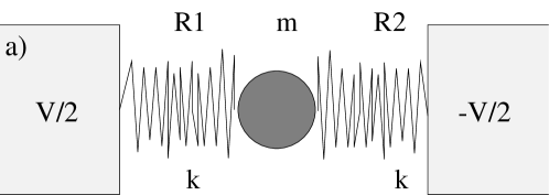
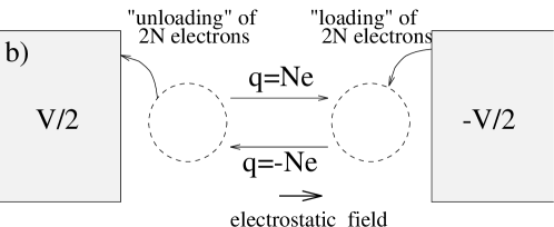
Figure 1: (a) Simple model of a soft Coulomb blockade system in which a metallic grain (center) is linked to two electrodes by elastically deformable organic molecular links. (b) Dynamic instabilities occur since in the presence of a sufficiently large bias voltage $V$ the grain is accelerated by the same electrostatic force towards first one, then the other electrode. A cyclic change in direction is caused by the repeated “loading” of electrons near the negatively biased electrode and the subsequent “unloading” of the same at the positively biased electrode. As a result the sign of the net grain charge alternates leading to an oscillatory grain motion and a novel “electron shuttle” mechanism for charge transport.

The purpose of the present paper is to carry the analysis presented in Ref. [8] quite a bit further. Strictly speaking the analytical part of the analysis in our earlier work is valid for low tunnel-barrier resistances when the rate of charge redistribution between grain and leads, inversely proportional to the tunneling resistance, is assumed to be so large in comparison with the vibration frequency that the stochastic fluctuations in grain charge during a single vibration period are unimportant. In order to describe the opposite limit of low charge redistribution frequencies characteristic of high-resistance tunnel barriers we develop here a new approach for considering the coupling betwen charge fluctuations and grain vibrations. We show that in the case of weak electromechanical coupling (i.e. when a change of the grain charge by $e$ does not significantly affect the vibrational motion) the main results which can be obtained within the model introduced in Ref. [8] can be proven to be correct even for high resistance junctions. In this high ohmic limit a new scenario for the shuttle instability becomes possible leading to hysteresis in the current - voltage characteristics.

The paper is organized as follows: In Section 2 we present our model composite Coulomb blockade system as well as a derivation of the equations governing the charge transport through the system. Then, in Section 3 we derive the dynamical equations for the case when the ‘fast’ grain oscillations have been averaged out so that only the ‘slow’ variation in oscillation amplitude remains. In Section 4 these equations are used to analyze the shuttle instability and the resulting current - voltage characteristics in our model Coulomb blockade system. The results are in good agreement with our earlier numerical results. The analytically solvable model is in addition useful for analyzing the nature of the loss of stability as the shuttle mechanism sets in. Such an analysis — supplemented by Monte Carlo simulations — is carried out in Section 5, where we find that depending on the resistances of the tunnel junctions the transition from the static regime to the shuttle regime can be associated either with smooth increase in the amplitude of the self-oscillations or with a jump in the amplitude at the transition. Adopting nomenclature from the theory of oscillations [9] we are dealing with either soft or hard excitation of self-oscillations, where hard excitation is associated with a hysteretic behavior of the current as the bias voltage is swept up and down. Finally, in Section 6 we present our conclusions.

2 Model System

In this Section we present a model of the simplest possible composite Coulomb blockade system that retains the properties of interest for us. It consists of one small metallic grain of mass $M$ connected by elastic molecular links to two bulk leads on either side, as shown in Fig. 1a. The electrostatic potential of the grain $\phi$ is a linear function of the grain charge $Q$ and the bias voltage ${V}$

$$\phi=\frac{Q}{C(X)}+a(X){V}\,,$$

where $X$ denotes the displacement of the grain from the equilibrium position in the centre of the system. This relation defines the capacitance $C(X)$ that appears in the theory. In a symmetric situation, as the one considered in this paper, $\phi(Q,{V},X)=\phi(Q,-{V},-X)$ and hence the coefficients $C(X)$ and $a(X)$ are even and odd functions of $X$ respectively. For small displacements we have $\phi\approx Q/C$, where $C=C(0)$. The magnitude of $C$ corresponds typically to the size of the grain. There are three different forces acting on the grain; a linear elastic restoring force $F_{el}=-kX$, a dissipative damping force $F_{d}=-\gamma_{d}\dot{X}$ and an electrostatic force $F_{q}=\frac{d}{dx}\mathcal{F}$,

$$\mathcal{F}\equiv U_{\mathrm{e}}-\frac{{V}}{2}(Q_{\mathrm{L}}-Q_{\mathrm{R}})\,,$$

where the electrostatic energy $U_{\mathrm{e}}$ of the system and the charges in the left (right) lead $Q_{\mathrm{L}}$ ($Q_{\mathrm{R}}$) are considered to be functions of $Q$ and ${V}$. The function $\mathcal{F}$ is bilinear in $Q$ and ${V}$ hence

$$\mathcal{F}=\frac{Q^{2}}{2C(X)}+\vartheta(X)Q{V}+\frac{{V}^{2}}{2}b(X)\,.$$

For a symmetric junction

$$\mathcal{F}(Q,{V},X)=\mathcal{F}(Q,-{V},-X)$$

implying that $\vartheta(X)$ is an odd function and that $C(X)$ and $b(X)$ are even. Then, for small displacements,

$$F_{q}=\frac{{V}}{L}Q,\mbox{ }L^{-1}\equiv\frac{d\vartheta(X)}{dX}{\Bigg{|}}_{X=0}$$

and one can consider $\mathcal{E}\equiv{V}/L$ as an effective electrostatic field induced by the bias voltage acting on the grain between the leads. This way we arrive at the estimate $L\sim$distance between the leads.

Knowing the forces that act on the grain, we may now introduce its equation of motion,

$$M\ddot{X}+\gamma_{d}\dot{X}+kX=\mathcal{E}Q(t)\,.$$ (1)

If the Coulomb charging energy, $U_{c}=e^{2}/C$, satisfies $U_{c}\gg\hbar/RC,\beta^{-1}$ where $R$ is the characteristic tunneling resistance and $\beta$ is the inverse temperature, one can expect a strong quantization of the charge $Q(t)$ in units of the elementary charge $e$,

$$Q(t)=en(t)\,,$$

where $n(t)$ will be a step function which can take on only integer values. Changes in $n(t)$ with time are due to quantum transitions of electrons between the grain and the leads. According to the ‘orthodox’ Coulomb blockade theory [2] the probability for the transition

$$(n,Q_{\mathrm{L,R}})\rightarrow(n\pm 1,Q_{\mathrm{L,R}}\mp e)$$

to occur during a small time interval $\Delta t$ when the grain is located at $X$ can be expressed as

$$\mathcal{W}_{\mathrm{L,R}}^{(\pm)}(n,X,\Delta t)=\Delta t\frac{1}{R_{\mathrm{L,R}}(0)C}\Gamma_{\mathrm{L,R}}^{(\pm)}(n,X)\,,$$ (2)

where

$$\Gamma_{\mathrm{L}}^{(\pm)}(n,X) = \left(\frac{R_{\mathrm{L}}(0)}{R_{\mathrm{L}}(X)}\right)f(\pm\frac{{V}C}{2e}\mp n-\frac{1}{2})$$

$$\Gamma_{\mathrm{R}}^{(\pm)}(n,X) = \left(\frac{R_{\mathrm{R}}(0)}{R_{\mathrm{R}}(X)}\right)f(\pm\frac{{V}C}{2e}\pm n-\frac{1}{2})\,.$$ (3)

Here the function $f$ is defined as

$$f(x)=\frac{x}{1-\exp({-\beta U_{c}x})}\,,$$ (4)

where $R_{\mathrm{L(R)}}(X)$ is the tunneling resistance of the left (right) junction which depends exponentially on the distance between the grain and the respective lead. In this paper $R_{\mathrm{L}}(X)=R_{\mathrm{R}}(-X)=R\exp(X/\lambda)$ where we refer to $\lambda$ as the tunneling length. Depending on the material of the reservoirs and the insulating links $\lambda$ can be estimated to lie within $0.05{\rm{\AA}}-3{\rm{\AA}}$ for direct tunneling from the electrodes to the grain. Due to the strong exponential dependence on the tunneling resistances the variations in capacitance with position are relatively small and are therefore neglected. The equations (1)-(4) hence define our model system.

3 Limit of Weak Electromechanical Coupling

In this Section we describe how the model system introduced above can be solved analytically for the case of weak electromechanical coupling. In later Sections this analytical solution will be compared to ‘exact’ Monte-Carlo results and found to be very useful in the further analysis of the model system. The key is to average over the fast grain oscillations so that we are left with a set of equations describing only the slow variations in the amplitude. We start by considering the typical scales of our parameters. It is natural to use $\lambda$ as a characteristic length scale. Furthermore the condition for observing Coulomb blockade effects requires that we operate with voltages ${V}$ of the order of the Coulomb blockade offset voltage ${V}_{0}=U_{c}/e=e/C$. Introducing the dimensionless variables $x\equiv X/\lambda$ and ${v}\equiv{V}/{V}_{0}$ the equation of motion for the grain (1) turns into

$$\ddot{x}+\omega^{2}x=\frac{\Omega^{2}}{2}{v}n(t)-\gamma\dot{x}\,,$$ (5)

where $\omega=\sqrt{k/M}$ is the elastic oscillation frequency and $\gamma$ and $\Omega^{2}$ are defined through $\gamma\equiv\gamma_{d}/M$ and

$$\Omega^{2}\equiv\frac{e^{2}}{MLC\lambda}=\frac{\lambda}{L}\frac{{U}_{c}}{E_{\mathrm{\lambda}}}\omega^{2}\,.$$

Here $E_{\mathrm{\lambda}}=k\lambda^{2}/2$ is the energy of harmonic mechanical vibrations with amplitude $\lambda$. For a nanoscale grain and typical organic junctions $\Omega^{2}/\omega^{2}=\epsilon\sim 10^{-2}$. Taking $\gamma/\omega$ to be of the same order we can separate out slow variations in oscillation amplitude by averaging over the fast oscillations. This is conveniently done by looking for a solution to (5) of the form

$$x(t)=\tilde{x}(t)\sin(\omega t)\,,$$ (6)

where $\tilde{x}(t)$ is a slowly varying function such that $\dot{\tilde{x}}(t)\sim\epsilon\omega$. Substituting (6) into (5), multiplying by $\cos(\omega t)$ and averaging over a time interval $T$ yields

$$\frac{\mathrm{d}\tilde{x}}{\mathrm{d}t}=\frac{\Omega^{2}}{2\omega}{v}\left\langle n(t)\cos(\omega t)\right\rangle_{\tilde{x}(t)}-\frac{1}{2}\gamma\tilde{x}(t)\,.$$ (7)

The time average is indicated by brackets and defined as

$$\left\langle g(t)\right\rangle_{\tilde{x}}=\frac{1}{T}\int_{t-T/2}^{t+T/2}g(\tau)\mathrm{d}\tau\,,$$

where the index $\tilde{x}$ indicates that the averaging process is performed for harmonic oscillations with constant amplitude $\tilde{x}$. The value of $T$ has to be chosen to obey the double inequality

$$\omega^{-1},\omega_{\mathrm{R}}^{-1}=RC\ll T\ll t_{\mathrm{S}}=\omega^{-1}\epsilon^{-1}\,,$$

where $t_{\mathrm{S}}\sim 10^{-9}-10^{-8}\mathrm{s}$ is the characteristic time for changes in the vibration amplitude $\tilde{x}(t)$ and $\omega_{\mathrm{R}}^{-1}\sim 10^{-10}\mathrm{s}$ is the typical time for charge redistribution between the leads and the grain. With this choice of $T$ the grain will perform many oscillations which differ very little in amplitude during the averaging, i.e.

$$\frac{\tilde{x}(t+T)-\tilde{x}(t)}{\tilde{x}(t)}\ll 1\,.$$

Introducing the dimensionless mechanical vibration energy

$$E(t)=\frac{M\omega^{2}(\lambda\tilde{x}(t))^{2}}{2E_{\mathrm{\lambda}}}$$

and making a change of variables in (7) we get

$$\frac{\mathrm{d}E}{\mathrm{d}t}={v}\frac{\Omega^{2}}{\omega}W(E)-\gamma E$$ (8)

$$W(E)=\sqrt{E}\left\langle n(t)\cos(\omega t)\right\rangle_{E}\,.$$ (9)

The physical meaning of the term containing $W(E)$ is that energy is pumped into the system when the grain is oscillating. Due to the correlation between the charge fluctuations $n(t)$ and the position of the grain, $x(t)=\sqrt{E(t)}\sin(\omega t)$, $W(E)$ will be nonzero. In order to describe this correlation we introduce the correlation function

$$P_{n}(\varphi,E)=\pi\left\langle\delta_{n,n(t)}\delta\left(\sin{\textstyle\frac{1}{2}}(\omega t-\varphi)\right)\right\rangle_{E}\,,$$ (10)

where the average is taken over a time $T$ that allows the grain to perform $N=T\omega/2\pi$ complete harmonic oscillations with constant energy $E$. The grain will now pass through the particular point

$$(E,\varphi)=(x,\dot{x})=(x_{E}(\varphi),\dot{x}_{E}(\varphi))=\left(\sqrt{E}\sin(\varphi),\omega\sqrt{E}\cos(\varphi)\right)$$

in a two-dimensional ‘phase space’ $N$ times and $P_{n}(\varphi,E)$ will thus be the relative number of times the grain passes this point with charge $Q=en$. Using the definition (10) of $P_{n}(\varphi,E)$ we rewrite (9) as

$$W(E)=\frac{\sqrt{E}}{2\pi}\int\mathrm{d}\varphi\cos(\varphi)q(\varphi,E)$$ (11)

$$q(\varphi,E)\equiv\sum_{n}nP_{n}(\varphi,E)\,.$$ (12)

In Appendix A it is shown how one can obtain a differential equation for $P_{n}(\varphi,E)$. The equations (8), (11) and (31) then completely describe the behavior of the model and are stated below in their final form,

$$\frac{\mathrm{d}E}{\mathrm{d}t} = {v}\frac{\Omega^{2}}{\omega}W(E)-\gamma E$$ (13)

$$W(E) = \frac{\sqrt{E}}{2\pi}\int\mathrm{d}\varphi\cos(\varphi)\sum_{n}nP_{n}(\varphi,E)$$ (14)

$$\frac{\d{\vec{P}}(\varphi,E)}{\d\varphi} = \nu_{\mathrm{R}}\hat{\mathcal{G}}(\sqrt{E}\sin\varphi)\vec{P}(\varphi,E)\,.$$ (15)

Here $\vec{P}(\varphi,E)$ is a vector containing $P_{n}(\varphi,E)$ and the components of the matrix $\hat{\mathcal{G}}$ appearing in (15) are

$$\hat{\mathcal{G}}_{n,m}(x_{E}(\varphi))=-\delta_{n,m}[\Gamma^{+}_{E}(n,\varphi)+\Gamma^{-}_{E}(n,\varphi)]+\delta_{n,m\pm 1}\Gamma^{\mp}_{E}(n,\varphi)$$

$$\Gamma_{\mathrm{E}}^{\pm}(n,\varphi)=\Gamma_{\mathrm{L}}^{\pm}(n,x_{E}(\varphi))+\Gamma_{\mathrm{R}}^{\mp}(n,x_{E}(\varphi))$$

and we have defined a dimensionless charge relaxation frequency,

$$\nu_{\mathrm{R}}=\frac{\omega_{\mathrm{R}}}{\omega}\,.$$

If we formally solve equations (13-15) any observable characterizing the system can be evaluated. One such observable is the average current through the left and rights leads respectively. In Appendix A this current is shown to be

$$\bar{I}_{\mathrm{L,R}}=\frac{e\omega}{2\pi}\int_{0}^{2\pi}\mathrm{d}\varphi\sum_{n}j_{n}^{\mathrm{L,R}}(\sqrt{E}\sin\varphi)P_{n}(\varphi,E)\,,$$ (16)

where

$$j_{n}^{\mathrm{L,R}}(\sqrt{E}\sin\varphi)=\nu_{\mathrm{R}}\mathrm{e}^{\mp\sqrt{E}\sin\varphi}\left[f({v}/2\mp n-1/2)-f(\pm n-{v}/2-1/2)\right].$$

(17)

By using the definition (17) of the partial currents and Eq. (12) together with (31) one comes to the expression

$$\frac{\d q(\varphi,E)}{\d\varphi}=\sum_{n}\left(j_{n}^{\mathrm{L}}(\sqrt{E}\sin\varphi)-j_{n}^{\mathrm{R}}(\sqrt{E}\sin\varphi)\right)P_{n}(\varphi,E)\,.$$ (18)

This form of our equations is especially useful when $v=(2n+1)$ at zero temperature, i.e. when the function $f(x)=x\theta(x)$ and when the voltage is chosen at the point where a new channel is about to switch on. The differential equation (18) for $q$ then simplifies to

$$\frac{\d q(\varphi,E)}{\d\varphi}=\nu_{\mathrm{R}}\left((1-{v})\sinh(\sqrt{E}\sin\varphi)-2q(\varphi,E)\cosh(\sqrt{E}\sin\varphi)\right).$$ (19)

Instead of $n$ coupled differential equations for $P_{n}$ there is now only one for $q(\varphi,E)$.

We are now ready to apply our analytical solution of the model Coulomb blockade system to an analysis of the shuttle instability. This will be done in the next two Sections.

4 Analytical and Numerical Analysis of the Shuttle Instability

In this Section we will use both the approximate analytical approach of the previous Section and an ‘exact’ numerical scheme to analyze the shuttle instability in our model Coulomb blockade system. Using first the analytical approach we conclude from Eq. (13) that the stationary regimes of our system are defined by

$$v\frac{\Omega^{2}}{\omega}W(E)=\gamma E\,.$$

This equation always has one trivial solution $E=0$. When this solution is stable it corresponds to the system being close to the point of mechanical equilibrium only subject to small deviations due to charge fluctuations. We will refer to this regime as the static regime. For our symmetric system the current-voltage characteristics in this regime show no pronounced Coulomb blockade structure even though there are peaks in the differential conductance due to the switching on of new channels at voltages $v_{n}=2n+1$ [1].

In Appendix B it is shown that for small $E$ we have

$$W(E)=\alpha(v){E}+\mathcal{O}(E^{2}),\mbox{ }\alpha(v)>0\,.$$

Hence, according to (13) the point $(x=0,\dot{x}=0)$ will become unstable if

$$\frac{\d E}{\d t}\Bigg{|}_{E=0}>0\mbox{ }\Leftrightarrow\mbox{ }v\frac{\Omega^{2}}{\omega}\alpha(v)>\gamma\,,$$

i.e. when more energy is pumped into the system than can be dissipated. We define the critical voltage $v_{c}$ as the voltage when

$$v_{c}\frac{\Omega^{2}}{\omega}\alpha(v_{c})=\gamma\,.$$

This equation cannot be solved for $v_{c}$ in the general case, but if we know $\alpha(v)$ for some specific values $v_{1}$ and $v_{2}$ of the bias voltage and if

$$v_{1}\frac{\Omega^{2}}{\omega}\alpha(v_{1})<\gamma<v_{2}\frac{\Omega^{2}}{\omega}\alpha(v_{2})\,,$$

it follows that $v_{c}$ lies in the interval $[v_{1},v_{2}]$ since $\alpha(v)$ is a continuous function of $v$. For the special case $v=v_{n}\equiv(2n+1)$ at zero temperature we only need to consider the single equation (19). By performing successive partial integrations of (14) using (19) and approximating $\sinh{x}\approx x$ and $\cosh x\approx 1$ one finds that

$$\alpha(v_{n})=\frac{\nu_{\mathrm{R}}(v_{n}-1)}{2(1+4\nu_{R}^{2})}\,.$$

Hence the critical voltage can be established within one Coulomb blockade voltage,

$$\left|v_{c}-2\left[\frac{3}{4}+\sqrt{\frac{\gamma\omega(1+4\nu_{\mathrm{R}}^{2})}{2\nu_{\mathrm{R}}\Omega^{2}}+\frac{1}{16}}\right]\right|<1$$ (20)

If this critical voltage is exceeded the oscillation amplitude will increase as the voltage is raised above $v_{c}$. The answer to the natural question whether this increase of amplitude will saturate at some definite value or not is determined by the behavior of $W(E)$ as $E$ tends to infinity. To investigate the behavior of $W(E)$ for large values of $E$ it is convenient to consider the contributions to $W(E)$ from three different regions in $(x,\dot{x})$- space; a “right”, a “left” and a “central” region, see Fig. 2.

Figure 2: Division of the phase space into three regions: ‘left’, ‘center’ and ‘right’. In the left and right regions the charge distribution on the grain is determined by the exchange with the corresponding lead. In the center region charge exchange with both leads contribute to the charge distribution.

The “right” region is defined as $x_{E}(\varphi)>x_{E}(\varphi_{0})\equiv\ln E$, where the rate of the charge exchange between the grain and the right lead dominates over the exchange with the left lead. Similarly the “left” region is defined as $x_{E}(\varphi)<-x_{E}(\varphi_{0})$ where the converse is true. The third region is the central region where $|x_{E}(\varphi)|<x_{E}(\varphi_{0})$. In a symmetric system the first two regions contribute equally to $W(E)$ and we need only consider the “left” region. For this case it is convenient to represent Eq. (15) for $\vec{P}(\varphi,E)$ in the form

$$\hat{\mathcal{G}}_{\mathrm{L}}\vec{P}=-\varepsilon(E)\tau_{\mathrm{R}}g(\varphi)\frac{\d\vec{P}}{\d\varphi}-\varepsilon^{2}(E)g^{2}(\varphi)\hat{\mathcal{G}}_{\mathrm{R}}\vec{P}\,,$$ (21)

where

$$\hat{\mathcal{G}}_{\mathrm{L,R}}=e^{\pm x}\hat{\mathcal{G}}(x)|_{x\gg 1},\mbox{ }\varepsilon(E)=\exp(-x_{E}(\varphi_{0}))=E^{-1}$$

$$g(\varphi)=\exp(\sqrt{E}(\sin\varphi_{0}+\sin\varphi))<1\,,$$

i.e. $\hat{\mathcal{G}}_{\mathrm{L,R}}$ describes the charge exchange with the corresponding lead when the grain is disconnected from the other lead. For large $E$ when $\varepsilon\ll 1$ one can develop a perturbation procedure to solve (21). For the ‘left’ region one finds the expansion

$$\vec{P}(\varphi)=\vec{P}^{\mathrm{L}}-\varepsilon^{2}(E)g^{2}\hat{\mathcal{G}}_{\mathrm{L}}^{-1}\hat{\mathcal{G}}_{\mathrm{R}}\vec{P}^{\mathrm{L}}+...\,,$$

where $\vec{P}^{\mathrm{L}}$, which satisfies the equation $\hat{\mathcal{G}}^{\mathrm{L}}\vec{P}^{\mathrm{L}}=0$, describes the charge distribution for a grain in thermal equilibrium with the left lead. Therefore the charge on the grain will saturate at the value $q^{\mathrm{L}}=\sum nP_{n}^{\mathrm{L}}$ and as a consequence the leading term does not depend on the position of the grain. This is why the contribution from the left (and right) region to $W(E)$ will decrase with increasing amplitude. The contribution from the central region is restricted by the upper limit $4x_{E}(\varphi_{0})\max\{q(\varphi)\}$. All the above considerations yield the inequality

$$W(E)<A\ln E+B\quad\mbox{when}\quad E\gg 1\,.$$

This inequality implies that at large amplitude the rate of dissipation, $\gamma E$, always exceeds the rate at which energy is pumped into the system leading to a final stationary state with the grain oscillating with a finite amplitude $E=E_{\mathrm{sh}}$ if $v>v_{c}$. This oscillating regime we refer to as the shuttle regime. A more sophisticated treatment reveals that

$$W(E)=2q^{\mathrm{L}}\ln E+\mathcal{O}(1)\mbox{ when }E\gg 1\,.$$

This leads to the following estimation for $E_{\mathrm{sh}}$ as a function of the bias voltage at $v=v_{c}$ at zero temperature when 2$q^{\mathrm{L}}\sim v$

$$E_{\mathrm{sh}}=\frac{\Omega^{2}v^{2}}{\omega\gamma}\ln\left(\frac{\Omega^{2}v^{2}}{\omega\gamma}\right)\,.$$

To support the preceeding discussion we have performed numerical simulations of the system. Figure 3 shows the charge on the grain as a function of its position in the shuttle regime.

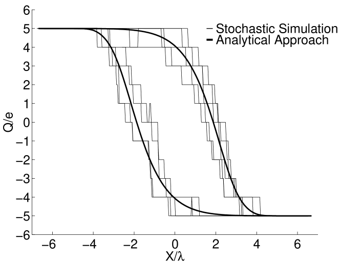
Figure 3: Comparison between ‘exact’ Monte Carlo simulations and the analytical approach. The graph shows the grain charge as a function of grain position in the shuttle regime at bias voltage $V=10V_{0}$ ($V_{0}$ is the theshold voltage for lifting the Coulomb blockade). The thin lines are from stochastic simulations and the thick smooth curve is the result of our analytical approach to the system. From this graph we see that the charging-decharging process takes place in the center of the system while the the charge on the grain saturates at it’s maximum (minimum) value outside this region.

The thin lines are the result of a Monte-Carlo simulation of the system when $v=10$ and the thick lines show the results of our analytical approach. The graph reveals the true stochastic nature of the charge on the grain as well as the validity of our analytical solution. Moreover one sees that the charging and decharging of the system takes place in a limited region around the center of the system while the charge saturates as the grain approaches the respective lead. To understand this behavior one can integrate Eq. (18) to get the following relationship for the charge on the grain

$$q(0)-q(\pi)=\int_{\pi}^{2\pi}\sum_{n}j_{n}^{\mathrm{L}}P_{n}(\varphi)\d\varphi-\int_{\pi}^{2\pi}\sum_{n}j_{n}^{\mathrm{R}}P_{n}(\varphi)\d\varphi$$

(Recall that $q(2\pi)=q(0)$ and that $q(0)$ [$q(\pi)$] is the charge on the grain as it passes the center position moving right [left]). Substituting this expression into (16) one can get the current in the form

$$\bar{I}=\frac{e\omega}{2\pi}[q(0)-q(\pi)]+\frac{e\omega}{2\pi}\int_{0}^{\pi}\d\varphi\sum_{n}j_{n}^{\mathrm{L}}P_{n}(\varphi)+\frac{e\omega}{2\pi}\int_{\pi}^{2\pi}\d\varphi\sum_{n}j_{n}^{\mathrm{R}}P_{n}(\varphi)\,.$$

(22)

The last two terms determine the current between the grain and the most distant lead. We can think of this contribution as a tunnel current through the central cross section of the system. The first term corresponds to the current through this cross section when the grain passes the point $x=0$. This current exists only because of the oscillatory motion of the grain. We refer to this mechanically mediated current as the shuttle current. At large amplitudes we can estimate the contribution from the last two terms in (22) to be of the order $1/\sqrt{E}$. At the same time it follows from a perturbative treatment analogous to the one carried out above to determine the behavior of $W(E)$ for large $E$ that

$$-q(\pi)=+q(0)=|q^{\mathrm{L}}|-\mathcal{O}\left(\frac{1}{\sqrt{E}}\right)\,.$$

At zero temperature we have also

$$|q^{\mathrm{L,R}}|=\left[\frac{v+1}{2}\right]$$

where the square brackets $[..]$ denotes the integer part of the argument. Thus we find for this case that

$$\bar{I}=\frac{e\omega}{\pi}\left[\frac{v+1}{2}\right]+e\omega_{\mathrm{R}}\mathcal{O}\left(\frac{1}{\sqrt{E}}\right)\,.$$ (23)

From (23) one finds that for large amplitude oscillations a pronounced steplike behavior in the current appears in the symmetric case in contrast to the ordinary static Coulomb blockade case. This behavior is also seen in numerical simulations of the system. In Fig. 4 the current-voltage characteristics has been calculated. As the voltage is raised above $v_{c}$ the current departs from the current obtained in a static double junction and distinct steps appear.

Figure 4: Current through the Coulomb blockade system in the static regime ($V<V_{c}$) and in the shuttle regime ($V>V_{c}$). As the system enters the shuttle regime the current (solid line) deviates from the current for a static double junction (dashed line). After the transition to the shuttle regime distinct steps as predicted by Eq. (23) can be seen in the current even though we are modelling a symmetric system. The current in this figure and subsequent ones is normalized to the frequency of harmonic oscillations to demonstrate that the step height in the shuttle regime is proportional to $\omega$. In order to make a comparison with the current in the static regime this current has been scaled by the same factor.

5 Soft and Hard Excitation of Self-Oscillations

We have in the previous Sections shown that the stationary point $(x=0,\dot{x}=0)$ will become unstable for certain voltages $v>v_{c}$ and that the system will reach a self-oscillating regime with well defined amplitude. In this Section we now show that the transition from the static regime to the shuttle regime can be associated with either soft or hard excitation of self-oscillations. The terminology is adopted from the theory of oscillatons [9]); in the case of soft excitation of self-oscillations the amplitude increases smoothly from zero at the transition point, while the oscillation amplitude jumps to a finite value in the case of hard excitation of self-oscillations. The former case occurs when $W^{\prime\prime}(0)<0$ and the latter when $W^{\prime\prime}(0)>0$.

Figure 5: Schematic energy diagram for the case $W^{\prime\prime}(0)<0$. The graph shows $W(E)$ for a fixed set of parameters for three different voltages along with the line $\gamma E$. When $v=v^{\prime}<v_{c}$ all the energy pumped into the system can be dissipated and the stationary point $\mathbf{O}$ is stable. When $v=v_{c}$ this point becomes unstable and at voltage $v=v^{\prime}>v_{c}$ the system will reach a limit cycle with oscillation amplitude $\propto\sqrt{E}$ determined by the intersection point $\mathbf{P}$.

We start with the case when $W^{\prime\prime}(0)<0$ then for small $E$ and $v-v_{c}\ll v_{c}$ we have

$$W(E)=[\alpha(v_{c})+\alpha^{\prime}(v_{c})(v-v_{c})]E-\beta E^{2}\mbox{ }\mbox{ }\alpha,\beta>0\,.$$

The energy at constant amplitude satisfies according to (13)

$$v\frac{\Omega^{2}}{\omega}[\alpha(v)-\beta E]=\gamma\,,$$

where $v_{c}\alpha(v_{c}){\Omega^{2}}/{\omega}=\gamma$. Hence, in the vicinity of the transition the amplitude of oscillation will increase smoothly as

$$\tilde{x}=\sqrt{E}=\sqrt{\left(\frac{\alpha(v_{c})+v_{c}\alpha^{\prime}(v_{c})}{\beta}\right)\frac{(v-v_{c})}{v_{c}}}\,.$$ (24)

The development of the instability can be understood from the diagrams in Fig. 5. The graph shows $W(E)$ for a fixed set of parameters for three different voltages along with the line $\gamma E$. When $v<v_{c}$ the dissipation is larger than the pumping of energy into the system and the stationary point $\mathbf{O}$ is stable. When $v=v_{c}$ this point becomes unstable and at voltage $v>v_{c}$ the system will reach a limit cycle with oscillation amplitude $\propto\sqrt{E}$ determined by the intersection point $\mathbf{P}$.

Figure 6: Schematic energy diagram for the case $W^{\prime\prime}(0)>0$. The graph shows $W(E)$ for a fixed set of parameters for four different voltages along with the line $\gamma E$. When $v<v_{c1}$ only $\mathbf{O}$ will be a stable stationary point. At $v=v_{c1}$ a second unstable stationary point $\mathbf{Q}_{1}$ appears. For $v_{c1}<v=v^{\prime}<v_{c2}$ we have two coexisting stable points $\mathbf{O}$ and $\mathbf{P^{\prime}}$ leading to the hysteretic behavior of the system discussed in the text. At $v=v_{c2}$ $\mathbf{O}$ will become unstable and the system is determined to be in the limit cycle with amplitude corresponding to energy $E_{2}$ at the intersection $\mathbf{Q}_{2}$. As $v$ is increased above $v_{c2}$, the only stable stationary point left is $\mathbf{P^{\prime\prime}}$ corresponding to a limit cycle with amplitude $\propto\sqrt{E}$.

When $W^{\prime\prime}(0)>0$ the shuttle instability develops in a completely different way. Consider the diagrams in Fig. 6; the graph shows $W(E)$ for a fixed set of parameters for four different voltages along with the line $\gamma E$. Consider now the system being located in $\mathbf{O}$ at a voltage $v<v_{c1}$. In this case the system is in the static regime and exhibits the same behavior as an ordinary double junction. As the voltage is increased above $v_{c1}$ a second stable stationary point $\mathbf{P^{\prime}}$ appears but the system cannot reach this point since $\mathbf{O}$ is still stable. At $v=v_{c2}$, $\mathbf{O}$ becomes unstable and the system “jumps” from $\mathbf{O}$ to $\mathbf{Q}_{2}$. This instability we refer to as hard since the amplitude changes abruptly from $E=0$ to $E=E_{2}$ as the voltage is raised above $v_{c2}$. Now consider the case when the system is originally in the stationary point $\mathbf{P^{\prime\prime}}$ and the voltage is lowered. At $v<v_{c2}$, $\mathbf{O}$ becomes stable but cannot be reached by the system until $v$ has dropped to $v=v_{c1}$. At $v_{c1}$ the point $\mathbf{Q}_{1}$ becomes unstable and the system will “jump” to $\mathbf{O}$. This transition is characterized by an abrupt drop in amplitude from $E_{1}$ to $E=0$ at $v=v_{c1}$. Since $v_{c1}<v_{c2}$ the system will obviously exhibit a hysteretic behavior in the transition region.

By using the simplified equation (19) for the charge valid at zero temperature and $v=2n+1$ one can develop a perturbation expansion for $q(\varphi)$ for small $E$. Solving the system to third order in $\sqrt{E}$ we find an expression for $W^{\prime\prime}(0)$

$$\frac{\d^{2}W(E)}{\d E^{2}}\Bigg{|}_{E=0}=\frac{\tau_{\mathrm{R}}(v-1)}{16(\tau_{\mathrm{R}}^{2}+4)^{2}}(\tau_{\mathrm{R}}^{2}-12)\,.$$ (25)

From this result follows that the instability is associated with soft excitation of self-oscillations if $\tau_{\mathrm{R}}=\nu_{\mathrm{R}}^{-1}<2\sqrt{3}$ and with hard excitation of self-oscillations if $\tau_{\mathrm{R}}=\nu_{\mathrm{R}}^{-1}>2\sqrt{3}$.

Monte Carlo simulations of the system support the existence of two different types of instabilities. In Fig. 7 the result of a simulation for the case when $\tau_{\mathrm{R}}<2\sqrt{3}$ is shown.

(a) (b)

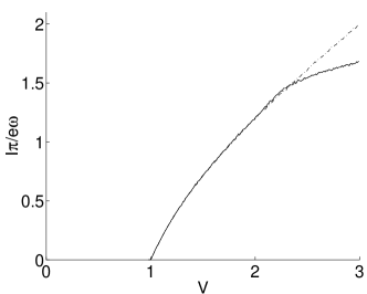
Figure 7: Soft excitation of self-oscillations from Monte Carlo simulations. (a) shows the root mean square amplitude as the voltage is raised above $V_{c}$ when $\tau_{\mathrm{R}}<2\sqrt{3}$. The predicted square-root increase of amplitude (Cf. Eq. (24)) can clearly bee seen here. The slight increase in amplitude before the transition comes from fluctuations in the charge on the grain. (b) The loss of stability is reflected in the current - voltage characteristics. As the system enters the shuttle regime the current deviates from the current seen in ordinary static double junctions (dashed line).

As expected the amplitude grows as in (24). The transition to the shuttle regime is visible in the current - voltage characteristics as a lowering of the current compared to the current for a static double junction. This decrease can be understood from the analytical expression (23) for the current .

A similar simulation for a case when $\tau_{\mathrm{R}}>2\sqrt{3}$ is shown in Fig. 8.

(a) (b)

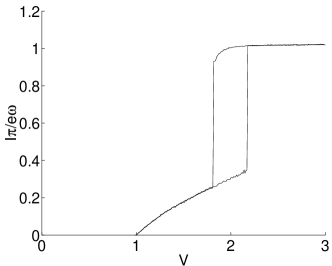
Figure 8: Hard excitation of self-oscillations from Monte Carlo simulations. (a) shows the root mean square amplitude at different voltages. As the voltage is raised from $V=0$ there is a discrete jump in amplitude at $V=V_{c2}$. Lowering the voltage again from $V=3V_{0}$ to zero reveals the hysteretic behavior as the amplitude drops to zero at $V=V_{c1}$. (b) The hysteretic behaviour is clearly visible in the current. Since $\nu_{\mathrm{R}}\ll 1$ the current in the shuttle regime lies very close to the value $I=e\omega/\pi$ as predicted in (23).

The predicted hysteretic behaviour is clearly visible along with the expected quantization of the current in the shuttle regime.

6 Conclusions

We have analyzed by both numerical and analytical methods charge transport by a novel ‘shuttle mechanism’ through the model shown in Fig. 1 of a self-assembled composite Coulomb blockade system [8]. A dynamical instability was found to exist above a critical bias voltage $V_{c}$, which depends on the junction resistances in the system. In this ‘shuttle regime’ there is a limit cycle in the position-charge plane for the grain (shuttle) motion as shown in Fig. 3. Above $V_{c}$ the current - voltage curve has a step-like structure, a type of Coulomb staircase, as shown in Fig. 4 even though we are modelling a symmetric double-junction system.

The transition from the static regime, where the grain does not move, to the shuttle regime can either be associated with soft excitation of self-oscillations, i.e. a continuous square-root increase in oscillation amplitude above $V_{c}$ as shown in Fig. 7 or by hard excitation of self-oscillations (the terminology is from the theory of oscillations [9]) implying a sudden jump in oscillation amplitude at an upper critical voltage $V_{c2}$. In the latter case the system behavior is hysteretic, as shown in Fig. 8; when the bias voltage is lowered the static regime is re-entered at a lower critical voltage $V_{c1}$.

Hard excitation of self-oscillation appears in our model for large junction resistances, $\tau_{R}\equiv RC>2\sqrt{3}/\omega$. At the same time the numerical value of $V_{c}\propto\sqrt{R}$ for large resistance junctions and may therefore be quite a bit larger than the threshold voltage $V_{0}$ for lifting the Coulomb blockade. The current in the high-voltage shuttle regime may furthermore be distinctly larger than in the static low-voltage regime. This is because it is governed mainly by the elastic vibration frequency of the grain and not by the rate of charge tunneling from the grain at rest in the center of the system, equally far from both leads. Hence in an experiment one might find a sudden increase of current at a quite large voltage $V_{c}$, where the shuttle mechanism sets in, rather than at the lower threshold voltage $V_{0}$, where the Coulomb blockade is lifted. This observation may be relevant in connection with the recent experiment by Braun et al. [3] where hysteresis effects in the current - voltage curves and an anomalously large threshold voltage (if interpreted within conventional Coulomb blockade theory) were reported for a system showing very large resistance at low bias voltages. The results of this work show that it may be possible to explain this experiment within a Coulomb blockade theory which allows for a shuttle instability of the type described here. In order to establish whether this mechanism is truly responsible for the behaviour of the system in [3] one has to study the experimental situation in great detail to properly estimate the mechanical parameters (elastic vibration frequency and damping) of the insulating material.

Appendix A Appendix A

In this Appendix we derive the differential equation (15) for the quantity $P_{n}(\varphi,E)$ defined in (10) and the result (16) for the average current $\bar{I}_{\mathrm{L,R}}$through the left and right leads.

Denote by $N_{n}(\varphi,E)=NP_{n}(\varphi,E)$ the number of times the grain passes through the point $(E,\varphi)$ carrying charge $Q=en$ and let
$N_{mn}(\varphi,E,\Delta t)$ be the number of times the grain has charge $Q=em$ as it passes through the point $(E,\varphi+\omega\Delta t)$ provided that it passed through $(E,\varphi)$ at a time $\Delta t$ earlier with charge $Q=en$, i.e.

$$N_{mn}(\varphi,E,\Delta t)=N\pi\left\langle\delta_{m,n(t+\Delta t)}\delta_{n,n(t)}\delta\left(\sin\left({\textstyle\frac{1}{2}}(\omega t-\varphi)\right)\right)\right\rangle_{E}$$ (26)

It’s now easy to see that

$$N_{n}(\varphi+\omega\Delta t,E) = \sum_{m}N_{nm}(\varphi,E,\Delta t)=\sum_{m\neq n}N_{nm}(\varphi,E,\Delta t)$$ (27)

$$+ \left(N_{n}(\varphi,E)-\sum_{m\neq n}N_{mn}(\varphi,E,\Delta t)\right)$$

Using the definition of $P_{n}(\varphi,E)$ in (27) yields

$$P_{n}(\varphi+\omega\Delta t,E) = \sum_{m\neq n}\frac{N_{nm}(\varphi,E,\Delta t)}{N_{m}(\varphi,E)}P_{m}(\varphi,E)$$ (28)

$$+ \left(P_{n}(\varphi,E)-\sum_{m\neq n}\frac{N_{mn}(\varphi,E,\Delta t)}{N_{n}(\varphi,E)}P_{n}(\varphi,E)\right)$$

For large $N$ the ratio $N_{nm}(\varphi,E,\Delta t)/N_{m}(\varphi,E)$ is the probability for the transition $(n,Q_{\mathrm{L,R}})\rightarrow(m,Q_{\mathrm{L,R}}\mp(m-n))$ during a small time interval $\Delta t$. But the probability for this kind of event was given in (2)

$$P_{n}(\varphi+\Delta\varphi,E) = \left(1-\sum_{\sigma=\pm}\sum_{\mathrm{S=L,R}}\mathcal{W}_{\mathrm{S}}^{\sigma}\left(n,x_{E}(\varphi),\frac{\Delta\varphi}{\omega}\right)\right)P_{n}(\varphi,E)$$ (29)

$$+ \sum_{\sigma=\pm}\sum_{\mathrm{S=L,R}}\mathcal{W}_{\mathrm{S}}^{\sigma}\left(n-\sigma 1,x_{E}(\varphi),\frac{\Delta\varphi}{\omega}\right)P_{n-\sigma 1}(\varphi,E)$$

We can write this as a first order differential equation if we introduce

$$\Gamma_{\mathrm{E}}^{\pm}(n,\varphi) = \Gamma_{\mathrm{L}}^{\pm}(n,x_{E}(\varphi))+\Gamma_{\mathrm{R}}^{\mp}(n,x_{E}(\varphi))$$ (30)

$$= \mathrm{e}^{-\sqrt{E}\sin\varphi}f(\pm\frac{v}{2}\mp n-\frac{1}{2})+\mathrm{e}^{\sqrt{E}\sin\varphi}f(\mp\frac{v}{2}\mp n-\frac{1}{2})$$

and use the relations (2) and (3)

$$\frac{\mathrm{d}P_{n}}{\mathrm{d}\varphi} = -\frac{\omega_{\mathrm{R}}}{\omega}\left(\Gamma_{\mathrm{E}}^{+}(n,\varphi)+\Gamma_{\mathrm{E}}^{-}(n,\varphi)\right)P_{n}(\varphi,E)$$ (31)

$$+ \frac{\omega_{\mathrm{R}}}{\omega}\left(\Gamma_{\mathrm{E}}^{-}(n+1,\varphi)P_{n+1}(\varphi,E)+\Gamma_{\mathrm{E}}^{+}(n-1,\varphi)P_{n-1}(\varphi,E)\right)$$

The average current through the left (right) lead can formally be written as

$$\bar{I}_{\mathrm{L,R}}=e\left\langle\frac{1}{\Delta t}\sum_{\sigma=\pm}\sigma\mathcal{W}_{\mathrm{L,R}}^{\sigma}\left(n(t),X(t),\Delta t\right)\right\rangle$$ (32)

Within our approximation we now consider this average when the grain is oscillating with a fixed amplitude $\lambda\sqrt{E}$ and arrive at the equation

$$\bar{I}_{\mathrm{L,R}} = \frac{e}{\Delta t}\int\mathrm{d}\varphi\sum_{n}\sum_{\sigma=\pm}\sigma\mathcal{W}_{\mathrm{L,R}}^{\sigma}\left(n,\lambda\sqrt{E}\sin\varphi,\Delta t\right){\textstyle\frac{1}{2}}\left\langle\delta_{n,n(t)}\delta(\sin{\textstyle\frac{1}{2}}(\omega t-\varphi))\right\rangle$$

By using the definition of the partial currents (17) one gets eq. (16).

Appendix B Appendix B

In this Appendix we prove that the function $W(E)$ is a linear function of $E$ for small $E$ with a positive coefficient.

For small $E$ we can expand (15) around $\sqrt{E}=0$ to obtain

$$\frac{\d{\vec{P}}(\varphi,E)}{\d\varphi}=\nu_{\mathrm{R}}\left(\hat{\mathcal{G}}_{0}+\sqrt{E}\sin\varphi\hat{\mathcal{G}_{1}}+...\right)\vec{P}(\varphi,E)$$ (34)

where

$$\hat{\mathcal{G}}_{0}=\hat{\mathcal{G}}(0)\mbox{ and }\hat{\mathcal{G}}_{1}\equiv\frac{\d\hat{\mathcal{G}}(x)}{\d x}\Bigg{|}_{x=0}$$ (35)

Expanding $\vec{P}(\varphi,E)$ in the same fashion

$$\vec{P}(\varphi,E)=\vec{P}^{(0)}+\sqrt{E}\vec{P}^{(1)}(\varphi)+...$$ (36)

and inserting this Ansatz into (34) we find that $\vec{P}^{(0)}$ is the solution to the homogenous equation

$$\hat{\mathcal{G}}_{0}\vec{P}^{(0)}=0$$ (37)

The correction to first order in $\sqrt{E}$, $\vec{P}^{(1)}(\varphi)$ is the solution to the equation

$$\left(\tau_{\mathrm{R}}\frac{\d}{\d\varphi}-\hat{\mathcal{G}}_{0}\right)\vec{P}^{(1)}(\varphi)=\hat{\mathcal{G}}_{1}\vec{P}^{(0)}\sin\varphi$$ (38)

this is a standard differential equation which can be solved to yield

$$\vec{P}^{(1)}(\varphi)=\frac{\nu_{\mathrm{R}}}{\hat{I}+\nu_{\mathrm{R}}^{2}\hat{\mathcal{G}}_{0}^{2}}\hat{\mathcal{G}}_{1}\vec{P}^{(0)}\cos\varphi+\hat{\mathcal{G}}_{0}\frac{\nu_{\mathrm{R}}^{2}}{\hat{I}+\nu_{\mathrm{R}}^{2}\hat{\mathcal{G}}_{0}^{2}}\hat{\mathcal{G}}_{1}\vec{P}^{(0)}\sin\varphi$$ (39)

where $\hat{I}$ denotes the identity matrix and the matrix divisions are symbolic for the multiplication whith the inverse operator. Recalling the expression (14) for $W(E)$ and introducing the vector $\hat{n}$ having components $n$ we find when inserting our expansion that we have to first order in $E$

$$W(E) = \frac{\sqrt{E}}{2\pi}\int\mathrm{d}\varphi\cos(\varphi)\hat{n}\cdot\vec{P}(\varphi,E)$$ (40)

$$= \frac{E}{2}\left(\hat{n}\cdot\frac{\nu_{\mathrm{R}}}{\hat{I}+\nu_{\mathrm{R}}^{2}\hat{\mathcal{G}}_{0}^{2}}\hat{\mathcal{G}}_{1}\vec{P}^{(0)}\right)+\mathcal{O}(E^{2})=\alpha{E}+\mathcal{O}(E^{2})$$

However, to get instability we require that $\alpha$ defined as

$$\alpha=\frac{1}{2\pi}\int\mathrm{d}\varphi\cos(\varphi)\sum_{n}nP_{n}^{(1)}(\varphi)$$ (41)

must obey $\alpha>0$. To show this consider the auxiliary equation

$$\left(\tau_{\mathrm{R}}\frac{\d}{\d\tau}-\hat{\mathcal{G}}_{0}\right)\vec{P}^{(1)}(\tau)=\hat{\mathcal{G}}_{1}\vec{P}^{(0)}g(\tau)$$ (42)

where $g(\tau)$ can be any non singular real valued function. We now define

$$q^{(1)}(\tau)=\sum_{n}nP^{(1)}(\tau)$$ (43)

and the functional $A\{g(\tau)\}$ as

$$A\{g(\tau)\}=\frac{\int_{-\infty}^{\infty}g^{\prime}(\tau)q^{(1)}(\tau)\d\tau}{\int_{-\infty}^{\infty}g^{2}(\tau)\d\tau}$$ (44)

Note that we have as a special case

$$\alpha=\frac{1}{2}{A\{g(\tau)=\sin\tau\}}$$ (45)

From the theory of linear response

$$q^{(1)}(\tau)=\int_{-\infty}^{\infty}\chi(\tau-\tau^{\prime})g(\tau^{\prime})\d\tau^{\prime}$$ (46)

where $\chi(\tau-\tau^{\prime})$ is the response function. Using (46) in conjunction with (44) one gets

$$A\{g(\tau)\}=\frac{\int\d\omega\mathrm{Im}\{\omega\chi(\omega)\}|g(\omega)|^{2}}{\int\d\omega|f(\omega)|^{2}}$$ (47)

where the Fourier transform is defined here as

$$g(\omega)=\int\d\tau\mathrm{e}^{\mathrm{i}\omega\tau}g(\tau)$$ (48)

Causality together with the requirement that $q^{(1)}(\tau)$ be real give two conditions

$$\mathrm{Im}\{\chi(\omega)\}\neq 0\mbox{ for }\omega\neq 0\mbox{ and }\mathrm{Im}\{\chi(-\omega)\}=\mathrm{Im}\{-\chi(\omega)\}$$

Since $\chi$ is odd and nonzero at $\omega=0$ we conclude that

$$\mathrm{sgn}\left(\mathrm{Im}\{\omega\chi(\omega)\}\right)=Const$$ (49)

However, the response function $\chi(\omega)$ is independent of the particular form of $g(\tau)$ and hence we have that

$$\mathrm{sgn}(\alpha)=\mathrm{sgn}\left(A\{\sin\tau\}\right)=\mathrm{sgn}\left(A\{g(\tau)\}\right)$$ (50)

To see that $\alpha>0$ consider the special choice of $g(\tau)$

$$g_{0}(\tau)=\left\{\begin{array}[]{cc}{0}&{|\tau|>T}\\ {-g_{0}\mathrm{sgn}(\tau)}&{|\tau|<T}\end{array}\right.$$ (53)

where $T\gg{\omega}/{\omega_{\mathrm{R}}}$. This choice of $g$ has a very simple physical meaning. At $\tau<-T$ the grain is immobile in the centre of the system carrying charge $q=0$. At $\tau=-T$ it instantanously jumps to a location close to the right lead and waits there long enough to acquire a negative charge $q=-q_{0}$. It then moves instantanously to the left lead and there gets the charge $q=+q_{0}$ and then moves back to the middle. This process yields

$$A\{g_{0}(\tau)\}=3q_{0}/2T>0$$ (54)

Hence we have shown that for small $E$

$$W(E)=\alpha{E}+\mathcal{O}(E^{2}),\mbox{ }\alpha>0$$ (55)

References

• [1] I. O. Kulik and R. I. Shekhter, Sov. Phys. JETP ${\bf 41}$, 308 (1975).
• [2] D. V. Averin and K. K. Likharev, in Mesoscopic Phenomena in Solids, edited by B. L. Altshuler, P. A. Lee, and R. A. Webb (Elsevier, Amsterdam, 1991), p.173.
• [3] E. Braun, Y. Eichen, U. Sivan, and G. Ben-Yoseph, Nature 391, 775 (1998).
• [4] R. P. Andres, T. Bein, M. Dorogi, S. Feng, J. I. Henderson, C. P. Kubiak, W. Mahoney, R. G. Osifchin, and R. Reifenberger, Science ${\bf 272}$, 1323 (1996).
• [5] D. L. Klein, J. E. B. Katari, R. Roth, A. P. Alivisatos, and P. L. McEuen Appl. Phys. Lett. ${\bf 68}$, 2574 (1996).
• [6] E. S. Soldatov, V. V. Khanin, A. S. Trifonov, S. P. Gubin, V. V. Kolesov, D. E. Presnov, S. A. Iakovenko, and G. B. Khomutov, JETP Lett. 64, 556 (1996).
• [7] O. Alvarez and R. Lattore Biophys.J. 21, 1, (1978); V. I. Pasechnic and T. Gyanik, Sov. Biophyzika 22, 941 (1977).
• [8] L. Y. Gorelik, A. Isacsson, M. V. Voinova, B. Kasemo, R. I. Shekhter, and M. Jonson, Phys. Rev. Lett. 80, 4526 (1998); Physica B (in press) (1998).
• [9] A. A. Andronov, A. A. Vitt, and S. E. Khaikin, Theory of Oscillators (Pergamon, Oxford, 1966), Ch. IX, §9.