Confinement and Quantization Effects
in Mesoscopic Superconducting Structures

Abstract

We have studied quantization and confinement effects in nanostructured superconductors. Three different types of nanostructured samples were investigated: individual structures (line, loop, dot), 1-dimensional (1D) clusters of loops and 2D clusters of antidots, and finally large lattices of antidots. Hereby, a crossover from individual elementary ”plaquettes”, via clusters, to huge arrays of these elements, is realized. The main idea of our study was to vary the boundary conditions for confinement of the superconducting condensate by taking samples of different topology and, through that, modifying the lowest Landau level $E_{LLL}(H)$. Since the critical temperature versus applied magnetic field $T_{c}(H)$ is, in fact, $E_{LLL}(H)$ measured in temperature units, it is varied as well when the sample topology is changed through nanostructuring. We demonstrate that in all studied nanostructured superconductors the shape of the $T_{c}(H)$ phase boundary is determined by the confinement topology in a unique way.

I Introduction

I.1 Confinement and Quantization

”Confinement” and ”quantization” are two closely interrelated definitions: if a particle is ”confined” then its energy is ”quantized”, and vice versa. According to the dictionary, to ”confine” means to ”restrict within limits”, to ”enclose”, and even to ”imprison”. A typical example, illustrating the relation between confinement and quantization, is the restriction of the motion of a particle by an infinite potential well of size $L_{A}$. Due to the presence of an infinite potential $U(x)$ (Fig. 1) for $x<0$ and $x>L_{A}$, the wave function $\Psi(x)$ describing the particle is zero outside the well: $\Psi=0$ for $x<0$ and $x>L_{A}$ and, in the region with $U(x)=0\>\>(0\leq x\leq L_{A})$, the solutions of the one-dimensional Schrödinger equation correspond to standing waves with an integer number $n$ of half wavelengths $\lambda$ along $L_{A}:n\>{\lambda}_{n}/2=L_{A}$.

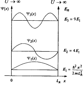
Figure 1: Confinement and quantization of the motion of a particle by an infinite potential well with size $L_{A}$ for $n$ = 1, 2 and 3.

This simple constraint results in the well-known quantized energy spectrum

$$E_{n}=\frac{\hbar^{2}k_{n}^{2}}{2m}=\frac{\hbar^{2}(2\pi/\lambda_{n})^{2}}{2m}=\frac{\hbar^{2}\pi^{2}}{2mL_{A}^{2}}n^{2}$$ (1)

Here $k_{n}$ is the wave number and $m$ is the free electron mass. To have an idea about the characteristic energy scales involved and their dependence upon the confinement length $L_{A}$, we have calculated (see Table 1) the energies $E_{1}$ (Eq. (1)) for electrons confined by an infinite potential well with the sizes $1$ Å, $1\>nm$ and $1\>\mu m$.

Table 1: Confinement by the infinite potential well

Confinement length $L_{A}$	Energy $E_{1}$	Temperature $T$
$1$ Å	$40\>eV$	$4\times 10^{5}\>K$
$1\>nm$	$0.4\>eV$	$4\times 10^{3}\>K$
$1\>\mu m$	$0.4\>\mu eV$	$4\>mK$

I.2 Nanostructuring

Recent impressive progress in nanofabrication has made it possible to realize the whole range of confinement lengths $L_{A}$ : from $1\>\mu m$ (photo-and e-beam lithography), via $1\>nm$ to $1$ Å (single atom manipulation) and, through that, to control the confinement energy (temperature) from a few $mK$ higher up to far above room temperature (Table 1).

This progress has stimulated dramatically the experimental and theoretical studies of different nanostructured materials and individual nanostructures. The interest towards such structures arises from the remarkable principle of ”quantum design”, when quantum mechanics can be efficiently used to tailor the physical properties of nanostructured materials.

Nanostructuring can also be considered as a sort of artificial modulation. We can identify then the main classes of nanostructured materials using the idea of their modification along one-, two- or three-axes, thus introducing 1-dimensional (1D)-, 2D- or 3D- artificial modulation (Fig. 2).

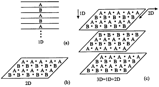
Figure 2: Schematic presentation of the vertical modulation in superlattices or multilayers (a), of the horizontal modulation achieved by a lateral repetition of elements A and B (b) and of the 1D+2D=3D artificial modulation (c).

The 1D or ”vertical” modulation represents then the class of superlattices or multilayers (Fig. 2a) formed by alternating individual films of two (A, B) or more different materials on a stack. Some examples of different types of multilayers are superconductor/insulator (Pb/Ge, WGe/Ge,…), superconductor/metal (V/Ag,…), superconductor/ferromagnet (Nb/Fe, V/Fe,…), ferromagnet/metal (Fe/Cr, Cu/Co,…), etc.

The ”horizontal” (lateral) superlattices (Fig. 2b) correspond to the 2D artificial modulation achieved by a lateral repetition of one (A), two (A,B) or more elements. As examples, we should mention here antidot arrays or antidot lattices, when A=microhole (”antidot”), or arrays and lateral superlattices consisting of magnetic dots.

If the 2D lateral modulation is applied to each individual layer of a multilayer or superlattice, then we deal with the 1D+2D=3D artificial modulation (Fig. 2c). For example, if arrays of antidots are made in a multilayer, then we have a system with 3D artificial modulation which combines 2D lateral ”horizontal” with the 1D ”vertical” modulation.

Finally, macroscopic nanostructured samples, with a huge number $N$ of repeated elementary ”plaquettes” (A,B,…), are examples of very complicated systems if the confined charge carriers or flux lines are strongly interacting with each other and the relevant interaction is of a long range. In this case the essential physics of such systems can be understood much better if we use clusters of elements ($N\simeq$ 10), instead of their huge arrays ($N\rightarrow\infty$) (Fig. 3).

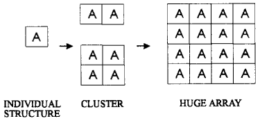
Figure 3: Schematic presentation of an individual structure, a cluster and a huge array.

These clusters, occupying an intermediate place between individual nanostructures ($N=1$) and nanostructured materials ($N\rightarrow\infty$), are very helpful model objects to study the interactions between flux lines or charge carriers confined by elements A. The ”growth” of clusters on the way from an individual object A to a huge array of A’s can be done either in a 1D or 2D fashion (Fig. 3), thus realizing 1D chains or 2D-like clusters of elements A.

I.3 Confining the Superconducting Condensate

The nanostructured materials and individual nanostructures, introduced in the previous section, can be prepared using the modern facilities for nanofabrication. It is worth, however, first asking ourselves a few simple questions like: why do we want to make such structures, what interesting new physics do we expect, and why do we want to focus on superconducting (and not, for example, normal metallic) nanostructured materials?

First of all, by making nanostructured materials, one creates an artificial potential in which charge carriers or flux lines are confined. The size $L_{A}$ of an elementary ”plaquette” A, gives roughly the expected energy scale in accordance with Table 1, while the positions of the elements A determine the pattern of the potential modulation. The concentration of charge carriers or flux lines can be controlled by varying a gate voltage (in 2D electron gas systems)Ensslin or the applied magnetic field (in superconductors)Pannetier84 . In this situation, different commensurability effects between the fixed number of elements A in an array and a tunable number of charge or flux carriers are observed.

Secondly, modifying the sample topology in nanostructured materials creates a unique possibility to impose the desired boundary conditions, and thus almost ”impose” the properties of the sample. A Fermi liquid or a superconducting condensate confined within such materials will be subjected to severe constraints and, as a result, the properties of these materials will be strongly affected by the boundary conditions.

While a normal metallic system should be considered quantum-mechanically by solving the Schrödinger equation:

$$\frac{1}{2m}\left(-\imath\hbar\vec{\nabla}-e\vec{A}\right)^{2}\Psi+U\>\Psi=E\>\Psi\>,$$ (2)

a superconducting system is described by the two coupled Ginzburg-Landau (GL) equations:

$$\frac{1}{2m^{\star}}(-i\hbar\vec{\nabla}-e^{\star}\vec{A})^{2}\Psi_{s}+\beta|\Psi_{s}|^{2}\Psi_{s}=-\alpha\Psi_{s}$$ (3)

$$\vec{j_{S}}=\vec{\nabla}\times\vec{h}=\frac{e^{\star}}{2m^{\star}}\left[\Psi_{s}^{\star}(-\imath\hbar\vec{\nabla}-e^{\star}\vec{A})\Psi_{s}+\Psi_{s}(\imath\hbar\vec{\nabla}-e^{\star}\vec{A})\Psi_{s}^{\star}\right]\>,$$ (4)

with $\vec{A}$ the vector potential which corresponds to the microscopic field $\vec{h}=rot\vec{A}/\mu_{0}$, $U$ the potential energy, $E$ the total energy, $\alpha$ a temperature dependent parameter changing sign from $\alpha>0$ to $\alpha<0$ as $T$ is decreased through $T_{c}$, ${\beta}$ a positive temperature independent constant, $m^{\star}$ the effective mass which can be chosen arbitrarily and is generally taken as twice the free electron mass $m$.

Note that the first GL equation (Eq. (3)), with the nonlinear term $\beta|\Psi_{s}|^{2}\Psi_{s}$ neglected, is the analogue of the Schrödinger equation (Eq. (2)) with $U$ = 0, when making a few substitutions: $\Psi_{s}\leftrightarrow\Psi$, $e^{\star}\leftrightarrow e$, $-\alpha\leftrightarrow E$ and $m^{\star}\leftrightarrow m$. The superconducting order parameter $\Psi_{s}$ corresponds to the wave function $\Psi$ in Eq. (2). The effective charge $e^{\star}$ in the GL equations is $2e$, i.e. the charge of a Cooper pair, while the temperature dependent GL parameter $\alpha$

$$-\alpha=\frac{\hbar^{2}}{2m^{\star}\>\xi^{2}(T)}$$ (5)

plays the role of $E$ in Schrödinger equation. Here $\xi(T)$ is the temperature dependent coherence length:

$$\xi(T)=\frac{\xi(0)}{\sqrt{1-\frac{T}{T_{c0}}}}.$$ (6)

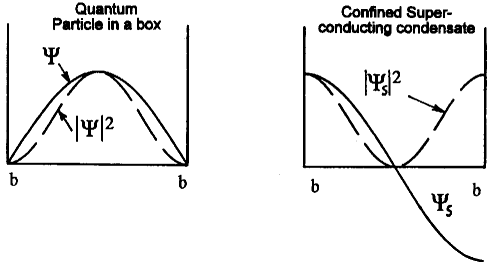
Figure 4: Boundary conditions for interfaces normal metal-vacuum and superconductor-vacuum.

The boundary conditions for interfaces normal metal-vacuum and superconductor-vacuum are, however, different (Fig. 4):

$$\left.\Psi\Psi^{\star}\right|_{b}=0$$ (7)

$$\left.(-\imath\hbar\vec{\nabla}-e^{\star}\vec{A})\Psi_{s}\right|_{\perp,b}=0$$ (8)

i.e. for normal metallic systems the density is zero, while for superconducting systems, the gradient of $\Psi_{s}$ (for the case $\vec{A}=0$) has no component perpendicular to the boundary. As a consequence, the supercurrent cannot flow through the boundary. The nucleation of the superconducting condensate is favored at the superconductor/ vacuum interfaces, thus leading to the appearance of superconductivity in a surface sheet with a thickness $\xi(T)$ at the third critical field $H_{c3}(T)$.

For bulk superconductors the surface-to-volume ratio is negligible and therefore superconductivity in the bulk is not affected by a thin superconducting surface layer. For nanostructured superconductors with antidot arrays, however, the boundary conditions (Eq. (8)) and the surface superconductivity introduced through them, become very important if $L_{A}\leq\xi(T)$. The advantage of superconducting materials in this case is that it is not even necessary to go to $nm$ scale (like for normal metals), since for $L_{A}$ of the order of 0.1-1.0 $\mu m$ the temperature range where $L_{A}\leq\xi(T)$, spreads over $0.01-0.1~{}K$ below $T_{c}$ due to the divergence of $\xi(T)$ at $T\rightarrow T_{c0}$ (Eq. (6)).

In principle, the mesoscopic regime $L_{A}\leq\xi(T)$ can be reached even in bulk superconducting samples with $L_{A}\sim$ $1~{}cm-1~{}m$, since $\xi(T)$ diverges. However, the temperature window where $L_{A}\leq\xi(T)$ is so narrow, not more than $\sim$ $1~{}nK$ below $T_{c0}$, that one needs ideal sample homogeneity and perfect temperature stability.

In the mesoscopic regime $L_{A}\leq\xi(T)$, which is quite easily realized in (perforated) nanostructured materials, the surface superconductivity can cover the whole available space occupied by the material, thus spreading superconductivity all over the sample. It is then evident that in this case surface effects play the role of bulk effects.

Using the similarity between the linearized GL equation (Eq. (3)) and the Schrödinger equation (Eq. (2)), we can formalize our approach as follows: since the parameter -$\alpha$ (Eqs. (3) and (5)) plays the role of energy $E$ (Eq. (2)), then the highest possible temperature $T_{c}(H)$ for the nucleation of the superconducting state in presence of the magnetic field $H$ always corresponds to the lowest Landau level $E_{LLL}(H)$ found by solving the Schrödinger equation (Eq. (2)) with ”superconducting” boundary conditions (Eq. (8)).

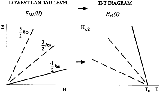
Figure 5: Landau level scheme for a particle in a magnetic field. From the lowest Landau level $E_{LLL}(H)$ the second critical field $H_{c2}(T)$ is derived (solid line).

Figure 5 illustrates the application of this rule to the calculation of the upper critical field $H_{c2}(T)$: indeed, if we take the well-known classical Landau solution for the lowest level in bulk samples $E_{LLL}(H)=\hbar\omega/2$, where $\omega=e^{\star}\mu_{0}H/m^{\star}$ is the cyclotron frequency. Then, from -$\alpha=E_{LLL}(H)$ we have

$$\frac{\hbar^{2}}{2m^{\star}\>\xi^{2}(T)}=\left.\frac{\hbar\omega}{2}\right|_{H=H_{c2}}$$ (9)

and with the help of Eq. (5), we obtain

$$\mu_{0}H_{c2}(T)=\frac{\Phi_{0}}{2\pi\xi^{2}(T)}$$ (10)

with $\Phi_{0}=h/e^{\star}=h/2e$ the superconducting flux quantum.

In nanostructured superconductors, where the boundary conditions (Eq. (8)) strongly influence the Landau level scheme, $E_{LLL}(H)$ has to be calculated for each different confinement geometry. By measuring the shift of the critical temperature $T_{c}(H)$ in a magnetic field, we can compare the experimental $T_{c}(H)$ with the calculated level $E_{LLL}(H)$ and thus check the effect of the confinement topology on the superconducting phase boundary for a series of nanostructured superconducting samples. The transition between normal and superconducting states is usually very sharp and therefore the lowest Landau level can be easily traced as a function of applied magnetic field. Except when stated explicitly, we have taken the midpoint of the resistive transition from the superconducting to the normal state, as the criterion to determine $T_{c}(H)$.

In this paper we present the systematic study of the influence of the confinement geometry on the superconducting phase boundary $T_{c}(H)$ in a series of nanostructured samples. We begin with individual nanostructures of different topologies (lines, loops, dots) (Section II) and then focus on ”intermediate” systems: clusters of loops fabricated in the form of a 1D chain of loops (Section III.A) or 2D antidot clusters (Section III.B). Finally, we move on to huge arrays of antidots in Section IV where we report on the $T_{c}(H)$ boundary for superconducting films with antidot lattices. The main emphasis of the paper is on the demonstration of the importance of the confinement geometry for the superconducting condensate and on the related quantization phenomena in nanostructured superconductors through the study of the phase boundaries $T_{c}(H)$.

II Individual structures: line, loop and dot

We begin this section by presenting the experimental results on the $T_{c}(H)$ phase boundary of individual superconducting mesoscopic structures of different topology. Simultaneously, we have kept other parameters of these samples, like material from which they are made (Al), the width of the lines ($w=0.15\>\mu m$) and the film thickness $t=25\>nm$ the same for all three structures, thus directly relating the differences in $T_{c}(H)$ to topological effects. The magnetic field $H$ is always applied perpendicular to the structures.

II.1 Line

In Fig. 6a the phase boundary $T_{c}(H)$ of a mesoscopic line is shown. The solid line gives the $T_{c}(H)$ calculated from the well-known formulaTin63 :

$$T_{c}(H)=T_{c0}\left[1-\frac{\pi^{2}}{3}\left(\frac{w\>\xi(0)\mu_{0}H}{\Phi_{0}}\right)^{2}\right]$$ (11)

which, in fact, describes the parabolic shape of $T_{c}(H)$ for a thin film of thickness $w$ in parallel magnetic field. Since the cross-section, exposed to the applied magnetic field, is the same for a film of thickness $w$ in a parallel magnetic field and for a mesoscopic line of width $w$ in a perpendicular field, the same formula can be used for bothVVM95 . Indeed, the solid line in Fig 6a is a parabolic fit of the experimental data with Eq. (11) where $\xi(0)=110\>nm$ was obtained as a fitting parameter. The coherence length obtained using this method, coincides reasonably well with the dirty limit value $\xi(0)=0.85(\xi_{0}\ell)^{1/2}=132\>nm$ calculated from the known BCS coherence length $\xi_{0}=1600\>nm$ for bulk AldGABook and the mean free path $\ell=15\>nm$, estimated from the normal state resistivity $\rho$ at $4.2\>K$Rom82 .

We can use also another simple argument to explain the parabolic relation $T_{c}(H)\propto H^{2}$: the expansion of the energy $E(H)$ in powers of $H$, as given by the perturbation theory, isWel38 :

$$E(H)=E_{0}+A_{1}LH+A_{2}SH^{2}+\cdots$$ (12)

where $A_{1}$ and $A_{2}$ are constant coefficients, the first term $E_{0}$ represents the energy levels in zero field, the second term is the linear field splitting with the orbital quantum number $L$ and the third term is the diamagnetic shift with $S$, being the area exposed to the applied field.

Now, for the topology of the line with a width $w$ much smaller than the Larmor radius $r_{H}\gg w$, any orbital motion is impossible due to the constraints imposed by the boundaries onto the electrons inside the line. Therefore, in this particular case $L=0$ and $E(H)=E_{0}+A_{2}SH^{2}$, which immediately leads to the parabolic relation $T_{c}\propto H^{2}$. This diamagnetic shift of $T_{c}(H)$ can be understood in terms of a partial screening of the magnetic field $H$ due to the non-zero width of the lineTinkham75 .

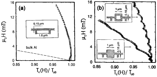
Figure 6: The measured superconducting/normal phase boundary as a function of the reduced temperature $T_{c}(H)/T_{c0}$ for a) the line, and b) the loop and the dot. The solid line in (a) is calculated using Eq. (11) with $\xi(0)=110\>nm$ as a fitting parameter. The dashed line represents $T_{c}(H)$ for bulk Al.

II.2 Loop

The $T_{c}(H)$ of the mesoscopic loop, shown in Fig. 6b, demonstrates very distinct Little-Parks (LP) oscillationsLitt62 superimposed on a monotonic background. A closer investigation leads to the conclusion that this background is very well described by the same parabolic dependence as the one which we just discussed for the mesoscopic lineVVM95 (see the solid line in Fig. 6a). As long as the width of the strips $w$, forming the loop, is much smaller than the loop size, the total shift of $T_{c}(H)$ can be written as the sum of an oscillatory part, and the monotonic background given by Eq. (11)VVM95 ; Gro68 :

$$T_{c}(H)=T_{c0}\left[1-\frac{\pi^{2}}{3}\left(\frac{w\>\xi(0)\mu_{0}H}{\Phi_{0}}\right)^{2}-\frac{\xi^{2}(0)}{R^{2}}\left(n-\frac{\Phi}{\Phi_{0}}\right)^{2}\right]$$ (13)

where $R^{2}=R_{1}\>R_{2}$ is the product of inner and outer loop radius, and the magnetic flux threading the loop $\Phi=\pi R^{2}\mu_{0}H$. The integer $n$ has to be chosen so as to maximize $T_{c}(H)$ or, in other words, selecting $E_{LLL}(H)$.

The LP oscillations originate from the fluxoid quantization requirement, which states that the complex order parameter $\Psi_{s}$ should be a single-valued function when integrating along a closed contour

$$\oint\vec{\nabla}\varphi\cdot dl=n\>2\pi\;\;\;\;\;\;\;\;\;\;\;\;\;\;\;\;n=\cdots\>,-2,-1,0,1,2,\>\cdots$$ (14)

where we have introduced the order parameter as $\Psi_{s}=|\Psi_{s}|\exp\>(\imath\varphi)$. Fluxoid quantization gives rise to a circulating supercurrent in the loop when $\Phi\neq n\Phi_{0}$, which is periodic with the applied flux $\Phi/\Phi_{0}$.

Using the sample dimensions and the value for $\xi(0)$ obtained before for the mesoscopic line (with the same width $w=0.15\>\mu m$), the $T_{c}(H)$ for the loop can be calculated from Eq. (13) without any free parameter. The solid line in Fig. 6b shows indeed a very good agreement with the experimental data. It is worth noting here that the amplitude of the LP oscillations is about a few $mK$ - in qualitative agreement with the simple estimate given in Table 1 for $L_{A}\simeq 1\>\mu m$.

Another interesting feature of a mesoscopic loop and other mesoscopic structures is the unique possibility they offer for studying nonlocal effectsStrN96 . In fact, a single loop can be considered as a 2D artificial quantum orbit with a fixed radius, in contrast to Bohr’s description of atomic orbitals. In the latter case the stable radii are found from the quasiclassical quantization rule, stating that only an integer number of wavelengths can be set along the circumference of the allowed orbits. For a superconducting loop, however, supercurrents must flow, in order to fulfil the fluxoid quantization requirement (Eq. (14)), thus causing oscillations of the critical temperature $T_{c}$ versus magnetic field $H$.

In order to measure the resistance of a mesoscopic loop, electrical contacts have, of course, to be attached to it, and as a consequence the confinement geometry is changed. A loop with attached contacts and the same loop without any contacts are, strictly speaking, different mesoscopic systems. This ”disturbing” or ”invasive” aspect can now be exploited for the study of nonlocal effectsStrN96 . Due to the divergence of the coherence length $\xi(T)$ at $T=T_{c0}$ (Eq. (6)) the coupling of the loop with the attached leads is expected to be very strong for $T\rightarrow T_{c0}$.

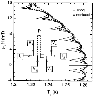
Figure 7: Local ($V_{1}/V_{2}$) and nonlocal phase boundaries ($V_{1}/V_{3}$ or $V_{2}/V_{4}$) $T_{c}(H)$. The mesuring current is sent through $I_{1}/I_{2}$. The solid and dashed lines correspond to the theoretical $T_{c}(H)$ of an isolated loop and a one-dimensional line, respectively. The inset shows a schematic of the structure, where the distance $P=0.4\>\mu m$.

Fig. 7 shows the results of these measurements. Both ”local” (potential probes across the loop $V_{1}/V_{2}$) and ”nonlocal” (potential probes aside of the loop $V_{1}/V_{3}$ or $V_{2}/V_{4}$) LP oscillations are clearly observed. For the ”local” probes there is an unexpected and pronounced increase of the oscillation amplitude with increasing field, in disagreement with previous measurements on Al microcylindersGro68 . In contrast to this, for the ”nonlocal” LP effect, the oscillations rapidly vanish when the magnetic field is increased.

When increasing the field, the background suppression of $T_{c}$ (Eq. (11)) results in a decrease of $\xi(T)$. Hence, the change of the oscillation amplitude with $H$ is directly related to the temperature-dependent coherence length. As long as the coherence of the superconducting condensate protuberates over the nonlocal voltage probes, the nonlocal LP oscillations can be observed.

On the other hand, the importance of an ”arm” attached to a mesoscopic loop, was already demonstrated theoretically by de Gennes in 1981dGA81 . For a perfect 1D loop (vanishing width of the strips) adding an ”arm” will result in a decrease of the LP oscillation amplitude, what we observed indeed at low magnetic fields, where $\xi(T)$ is still large. With these experiments, we have proved that adding probes to a structure considerably changes both the confinement topology and the phase boundary $T_{c}(H)$.

II.3 Dot

The Landau level scheme for a cylindrical dot with ”superconducting” boundary conditions (Eq. (8)) is presented in Fig. 8. Each level is characterized by a certain orbital quantum number $L$ where $\Psi_{s}=|\Psi_{s}|\exp\>(\mp\imath L\varphi)$PME96 . The levels, corresponding to the sign ”+” in the argument of the exponent are not shown since they are situated at energies higher than the ones with the sign ”-”. The lowest Landau level in Fig. 8 represents a cusp-like envelope, switching between different $L$ values with changing magnetic field. Following our main guideline that $E_{LLL}(H)$ determines $T_{c}(H)$, we expect for the dot the cusp-like superconducting phase boundary with nearly perfect linear background. The measured phase boundary $T_{c}(H)$, shown in Fig. 6b, can be nicely fitted by the calculated one (Fig. 8), thus proving that $T_{c}(H)$ of a superconducting dot indeed consists of cusps with different $L$’sBui90 . Each fixed $L$ describes a giant vortex state which carries $L$ flux quanta $\Phi_{0}$. The linear background of the $T_{c}(H)$ dependence is very close to the third critical field $H_{c3}(T)\simeq 1.69\>H_{c2}(T)$Saint-James65 . Contrary to the loop, where the LP oscillations are perfectly periodic, the dot demonstrates a certain aperiodicityVVMScripta , in very good agreement with the theoretical calculationsBui90 ; Benoist .

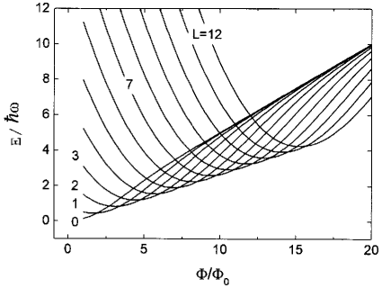
Figure 8: Energy level scheme versus normalized flux $\Phi/\Phi_{0}$ for a superconducting cylinder in a parallel magnetic field. The cusp-like $H_{c3}(T)$ line is formed due to the change of the orbital quantum number $L$.

III Clusters of loops and antidots

III.1 1D Clusters of loops

Figure 9: AFM micrographs of the studied structures: a) the bola, b) the double loop, and c) the triple loop.

After the description of the confinement effects of several individual superconducting structures (A = line, loop, dot) we are ready to move further on to clusters of elements A (Fig. 3) on our way from ”single plaquette” samples to materials nanostructured by introducing huge arrays of elements A. First we take A = loop and consider one-dimensional multiloop structures: ”bola”, double and triple loop Al structures. Figure 9 shows a AFM image of the structures. For these geometries some interesting theoretical predictions have been made, for which no experimental verification has been carried out up to know (see more in Ref.Bru96 ). The loops in all three structures have the same dimensions, thus leading to the same magnetic field period $\mu_{0}\Delta H=1.24\>mT$. The strips forming the structures are $0.13\>\mu m$ wide and the film thickness $t=34\>nm$. In all the experimental data we show, the parabolic background (Eq. (11)) is already subtracted in order to allow for a direct comparison with the theory. In the temperature interval where we measured the $T_{c}(H)$ boundary, the coherence length $\xi(T)$ is considerably larger than the width $w$ of the strips. This makes it possible to use the one-dimensional models for the calculation of $E_{LLL}(H)$ and thus $T_{c}(H)$. The basic idea is to consider $|\Psi_{s}|$ = constant across the strips forming the network and to allow a variation of $|\Psi_{s}|$ only along the strips. In the simplest approach $|\Psi_{s}|$ is assumed to be spatially constant (London limit (LL))Halevi83 ; Chi92 , in contrast to the de Gennes-Alexander (dGA) approachdGA81 ; Alex83 ; FinkBola , where $|\Psi_{s}|$ is allowed to vary along the strips. In the latter approach one imposes:

$$\sum_{n}\left(\imath\frac{\partial}{\partial x}+\frac{2\pi}{\Phi_{0}}A_{\parallel}(x)\right)\Psi_{s}(x)=0$$ (15)

at the points where the current paths join. The summation is taken over all strips connected to the junction point. Here, $x$ is the coordinate defining the position on the strips, and $A_{\parallel}$ is the component of the vector potential along $x$. Eq. (15) is often called the generalized first Kirchhoff law, ensuring current conservationFinkBola . The second Kirchhoff law for voltages in normal circuits is now replaced by the fluxoid quantization requirement (Eq. (14)), which should be fulfilled for each closed contour around a loop.

In Figs. 10-12 the phase boundaries of the three structures are shown. The dashed lines are the phase boundaries obtained with the LL, while the solid lines give the results from the dGA approach. As we discussed in Section II.B for a mesoscopic loop, attaching contacts modifies the confinement topology, so that the amplitude of the local LP oscillations is lowered at low magnetic fields. Here as well, the inclusion of the leads reduces the amplitude of the oscillations. The dash-dotted line in Figs. 10-12 give the result of the dGA calculation where the presence of the leads has been included. The values for $\xi(0)$ obtained from the fits agree within a few percent with the $\xi(0)$ values found independently from the monotonic background of $T_{c}(\Phi)$ (see Eq. (11)).

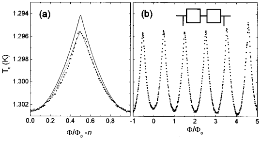
Figure 10: Experimental $T_{c}(\Phi)$ data for the bola with the parabolic background (Eq. (11)) subtracted. The dots are the experimental data points, while the lines correspond to the different theoretical results as explained in the text. a) Single period of $T_{c}(\Phi)$, b) A few periods of the experimental $T_{c}(\Phi)$ curve.

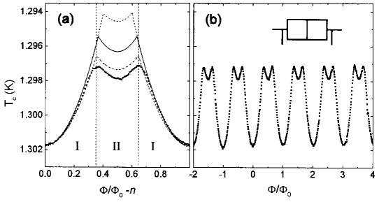
Figure 11: Experimental $T_{c}(\Phi)$ data for the double loop with the parabolic background (Eq. (11)) subtracted. The dots are the experimental data points, while the lines correspond to the different theoretical results as explained in the text. a) Single period of $T_{c}(\Phi)$, b) A few periods of the experimental $T_{c}(\Phi)$ curve.

First, in Fig. 10, we consider the mesoscopic ”bola” - two loops connected by a wire. Fink et al.FinkBola showed that, in the complete magnetic flux interval, the spatially symmetric solution, with equal orientation of the supercurrents in both loops, has a lower energy than the antisymmetric solution. Coming back to the similarity between a mesoscopic loop and a hydrogen atom, we discussed in Section II.B, we can then compare the bola with a $H_{2}$ molecule, where the symmetric and the antisymmetric solutions correspond to singlet and triplet states, respectively. In fact, $T_{c}(\Phi)$ of the bola is the same as for a single loop provided that the length of the strip connecting the two loops is short, as confirmed by the LP oscillations observed in the experimental $T_{c}(\Phi)$ (Fig. 10).

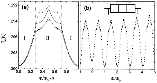
Figure 12: Experimental $T_{c}(\Phi)$ data for the triple loop with the parabolic background (Eq. (11)) subtracted. The dots are the experimental data points, while the lines correspond to the different theoretical results as explained in the text. a) Single period of $T_{c}(\Phi)$, b) A few periods of the experimental $T_{c}(\Phi)$ curve.

In what follows we will focus on the phase boundaries of the double (Fig. 11) and the triple loop (Fig. 12). To facilitate the discussion we divide the flux period in two intervals: flux regime I for $\Phi/\Phi_{0}<{\it g}$ or $\Phi/\Phi_{0}>(1-{\it g})$ and flux regime II for ${\it g}<\Phi/\Phi_{0}<(1-{\it g})$. In the flux regime I the phase boundaries, predicted by the different models, are nearly identical. Near $\Phi/\Phi_{0}=1/2$ (flux regime II), however, clear differences are found between the dGA approach and the LL. The dGA result fits better the experimental data with respect to the crossover point g between regimes I and II, and the amplitude of the $T_{c}$ oscillations. Using the dGA approach we have calculated the spatial modulation of $|\Psi_{s}|$ and the supercurrents for different values at the $T_{c}(\Phi)$ boundary. In the flux regime I $|\Psi_{s}|$ varies only slightly and therefore the results of the LL and the dGA models nearly coincide. The elementary loops have an equal fluxoid quantum number (and consequently an equal supercurrent orientation) for both the double and the triple loop geometry. For the double loop this leads to a cancellation of the supercurrent in the middle strip, while for the triple loop structure the fluxoid quantization condition (Eq. (14)) results in a different value for the supercurrent in the inner and the outer loops. As a result, the common strips of the triple loop structure carry a finite current.

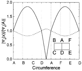
Figure 13: Calculated variation of $|\Psi_{s}|$ along the circumference of the double loop, at the phase boundary ($\Phi/\Phi_{0}=0.36$). The dashed line is the solution with $|\Psi_{s}|$ nearly spatially constant, while the solid line is the state with a node in the center of the strip connecting points $A$ and $D$.

In the flux regime II, qualitatively different states are obtained from the LL and the dGA approach: the states calculated within the dGA approach have strongly modulated $|\Psi_{s}|$ along the strips. This is most severe for the double loop: $\Psi_{s}$ shows a node ($|\Psi_{s}|=0$) in the center of the common strip, the phase $\varphi$ having a discontinuity of $\pi$ at this point. This node is a one-dimensional analog of the core of an Abrikosov vortex, where the order parameter also vanishes and the phase shows a discontinuity. In Fig. 13 the spatial variation of $|\Psi_{s}|$ along the strips is shown for $\Phi/\Phi_{0}=0.36$ close to the crossover point g. The dashed curve gives $|\Psi_{s}|$ in flux regime I, which is quasi-constant. The strongly modulated solution, which goes through zero in the center, is indicated by the solid line. Although there exists a finite phase difference across the junction points of the middle strip, no supercurrent can flow through the strip due to the presence of the node. This node is predicted to persist when moving below the phase boundary into the superconducting stateAmm95 ; Cas95 . Already in 1964 ParksPar64 anticipated that, in a double loop, ”a part of the middle link will revert to the normal phase”, and that ”this in effect will convert the double loop to a single loop”, giving an intuitive explanation for the maximum in $T_{c}(\Phi)$ at $\Phi/\Phi_{0}=1/2$. Such a modulation of $|\Psi_{s}|$ is obviously excluded in the LL, where the loop currents have an opposite orientation and add up in the central strip, thus giving rise to a rather high kinetic energy. An extra argument in favor of the presence of the node is given by the much better agreement for the crossover point g when the presence of the leads is taken into account in the calculations (see dash-dotted line in Fig. 11).

For the triple loop structure the modulation of $|\Psi_{s}|$ is still considerable in flux regime II, but it does not show any nodes. Therefore the supercurrent orientations can be found from the fluxoid quantum numbers $\{n_{i}\}$, obtained from integrating the phase gradients along each individual loop. When passing through the crossover point between flux regime I and regime II only the supercurrent in the middle loop is reversed, while increasing the flux above $\Phi/\Phi_{0}=1/2$ implies a reversal of the supercurrent in all loops.

Surprisingly, the behavior of a microladder with a linear arrangement of $m$ loops appears to be qualitatively different for even and for odd $m$ in the sense that $m$ determines the presence or absence of nodes in the common strips. For an infinitely long microladder $|\Psi_{s}|$ was found to be spatially constant below a certain $\Phi<\Phi_{c}$Sim82 , which is analogous to the states we find in flux regime I. For fluxes $\Phi>\Phi_{c}$ modulated $|\Psi_{s}|$ states, with an incommensurate fluxoid pattern, were found. At $\Phi/\Phi_{0}=1/2$, nodes appear at the center of every second common (transverse) branch.

III.2 2D clusters of antidots

As a 2D intermediate structure between individual elements A and their huge arrays (Fig. 3), we have studied the superconducting micro-square with a 2$\times$2 antidot cluster. In this case A= ”antidot”.

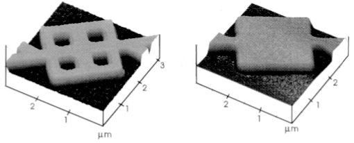
Figure 14: AFM image of the Pb/Cu 2$\times$2 antidot cluster (on the left) and of the reference sample (on the right).

The micro-square with the 2$\times$2 antidot cluster consists of a 2$\times$2 $\mu m^{2}$ superconducting square with four antidots (i.e. square holes of 0.53 $\times$ 0.53 $\mu m^{2}$). A Pb/Cu bilayer with $50\>nm$ of Pb and $17\>nm$ of Cu was used as the superconducting film for the fabrication of this structure. The thin Cu layer was deposited on the Pb to protect it from oxidation and to provide a good contact-layer for the wire-bounding to the experimental apparatus. An AFM image of the Pb/Cu 2$\times$2 antidot cluster, is shown in Fig. 14 together with a reference sample (i.e. a Pb/Cu micro-square of 2$\times$2 $\mu m^{2}$ without antidots). The Pb($50\>nm$)/Cu($50\>nm$) bilayer behaves as a Type II superconductor with a $T_{c0}=6.05\>K$, a coherence length, $\xi(0)\approx 35\>nm$ and a dirty limit penetration depth, $\lambda(0)\approx 76\>nm$. The $T_{c}(H)$ measurements on the reference sample revealed characteristic features originating from the confinement of the superconducting condensate by the dot geometry (see Section II.C). The additional features observed in the $T_{c}(H)$ phase boundary of the antidot cluster can therefore be attributed to the presence of the antidots.

The experimental $T_{c}(H)$ phase boundary is shown in Fig. 15. It was measured by keeping the sample resistance at 10% of its normal state value and varying the magnetic field and temperaturePuig97 .

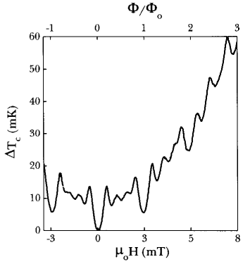
Figure 15: Experimental phase boundary, $\Delta T_{c}(H)$ for the Pb/Cu 2$\times$2 antidot cluster.

Strong oscillations are observed with a periodicity of 26 G and in each of these periods, smaller dips appear at approximately 7.5 G, 13 G and 18 G. The parabolic background superimposed on $T_{c}(H)$ can again be described by Eq. (11).

Defining a flux quantum per antidot as $\Phi_{0}=h/2e=BS$, where $B=\mu_{0}H$ and $S$ is an effective area per antidot cell ($S$= 0.8 $\mu m^{2}$), the minima observed in the magnetoresistance and the $T_{c}(H)$ phase boundary at integer multiples of 26 G can be correlated with a magnetic flux quantum per antidot cell, $\Phi=n\Phi_{0}$. The ones observed at 7.5 G, 13 G and 18 G correspond to the values $\Phi/\Phi_{0}$=0.3, 0.5 and 0.7.

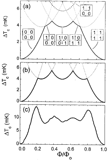
Figure 16: (a) Theoretical phase boundary, $T_{c}(\Phi/\Phi_{0})$, calculated in the London limit of the Ginzburg-Landau theory without any fitting parameter (solid line). All possible parabolic solutions are represented by dotted lines. The dashed line indicates the non-stable parallel configuration. The schematic representation of the $\{n_{i}\}$ quantum numbers at the antidots and characteristic current flow patterns for each parabolic branch are also sketched. (b) The $T_{c}(\Phi/\Phi_{0})$ phase boundary, calculated as in Fig. 16a , but with the curvature ”$\gamma$” of the parabolae taken as a free parameter. The $\gamma$-value was increased by a factor of two with respect to its calculated value used in Fig. 16a. (c) First period of the measured phase boundary shown in Fig. 15 after subtraction of the parabolic background.

The solutions obtained from the London model (LL) define a phase boundary which is periodic in $\Phi$ with a periodicity of $\Phi_{0}$. Within each parabola $\Delta T_{c}=\gamma(\Phi/\Phi_{0})^{2}$, where the coefficient $\gamma$ characterizes the effective flux penetration trough the unit cell. The $\gamma$-value is determined by the combination of $\lambda$ and the effective size of the current loops. In Fig. 16, the first period of this phase boundary, $\Delta T_{c}(\Phi)=T_{c0}-T_{c}(\Phi)$ versus $\Phi/\Phi_{0}$ is shown. Note that there are six parabolic solutions given by a different set of flux quantum numbers $\{n_{i}\}$, each one defining a specific vortex configuration. In Fig. 16a, this is indicated by the numbers shown inside the schematic drawings of the antidot cluster. Note that some vortex configurations are degenerate.

From all these possible solutions, for each particular value of $\Phi/\Phi_{0}$, only the branch with a minimum value of $\Delta T_{c}(\Phi)$ is stable (indicated with a solid line in Fig. 16a). Note that for the phase boundary, calculated within the 1D model of 4 equivalent and properly attached squares, no fitting parameters were used since the variation of $T_{c}(\Phi)$ was calculated from the known values for $\xi$ and the size. One period of the phase boundary of the antidot cluster is composed of five branches and in each branch a different stable vortex configuration is permitted. For the middle branch (0.37$<\Phi/\Phi_{0}<$0.63), the stable configuration is the diagonal vortex configuration (antidots with equal $n_{i}$ at the diagonals) instead of the parallel state (dashed line in Fig. 16a).

The net supercurrent density distribution circulating in the antidot cluster for different values of $\Phi/\Phi_{0}$ has been determined using the same approach. Circular currents flow around each antidot. For the states $n_{i}$=0 and $n_{i}$=1 currents flow in the opposite direction, since currents corresponding to $n_{i}$=0 must screen the flux to fulfil the fluxoid quantization condition (Eq. (14)), whereas for $n_{i}$=1 they have to generate flux. At low values of $\Phi/\Phi_{0}$, currents are canceled in the internal strips and screening currents only flow around the cluster. When we enter the field range corresponding to the second branch of the phase boundary, a vortex ($n_{i}$=1) is pinned around one antidot of the cluster (see Fig. 16a). At the third branch, the second vortex enters the structure and is localized in the diagonal. In the fourth branch of the phase boundary the third vortex is pinned in the antidot cluster. And finally, the current distribution for the fifth branch is similar to that of the first branch although currents flow in opposite direction.

Figure 16c shows the first period of the measured phase boundary $T_{c}(\Phi)$ after subtraction of the parabolic background. For all measured samples, the first period of the experimental phase boundary is composed of five parabolic branches with minima at $\Phi/\Phi_{0}$ = 0, 0.3, 0.5, 0.7, 1. If we compare it with the theoretical prediction given in Figure 16a, the overall shape can be reproduced although the experimental plot has two major peaks at $\Phi/\Phi_{0}$ = 0.2 and 0.8 whereas the theoretical curve only predicts cusps around these positions.

The agreement between the measured and the calculated $T_{c}(\Phi)$ is improved if we assume that the coefficient $\gamma$ can be considered as a fitting parameter. This seems to be feasible if we take into account the simplicity and limitation of the used 1D model. Due to the relatively large width of the strips forming the 2$\times$2 cluster, the sizes of the current loops can change since they are ”soft” in this case and not defined very precisely.

As a result, the coefficient $\gamma$ can not be treated as a known constant. If we use it as a free parameter (Fig. 16b) then the curvature of all parabolae forming $T_{c}(H)$ can be changed and the calculated $T_{c}(H)$ curve becomes closer to the experimental one though the amplitude of the maxima at $\Phi/\Phi_{0}$ = 0.2 and 0.8 is still lower than in the experiment (Fig. 16c). The discrepancy in the description of the amplitude of the maxima at $\Phi/\Phi_{0}$= 0.2 and 0.8 could also be related to the pinning of vortices by the antidot cluster when potential barriers between different vortex configurations may appear. At the same time, the achieved agreement between the positions of the measured and calculated minima of the $T_{c}(H)$ curves confirms that the observed effects are due to fluxoid quantization and formation of certain stable vortex configurations at the antidots.

IV Superconducting films with an antidot lattice

Laterally nanostructured superconducting films having regular arrays of antidots are convenient model objects to study the effects of the confinement topology on the $T_{c}(H)$ phase boundary in two different regimes. The first (or ”collective”) regime corresponds to the situation where all elements A, forming an array, are coupled.

From the experimental $T_{c}(H)$ data on antidot clusters we expect for films with an antidot lattice, higher critical fields at $\Phi=n\Phi_{0}$, which is in agreement with the appearance of the $T_{c}(H)$ cusps at $\Phi=n\Phi_{0}$ in superconducting networks Pannetier91 . Here, the flux $\Phi$ is calculated per unit cell of the antidot lattice.

On the other hand, by applying sufficiently high magnetic fields, the individual circular currents flowing around antidots, can be decoupled and the crossover to a ”single object” behaviour could be observed. In this case the relevant area for the flux is the area of the antidot itself and we deal with surface superconductivity around an antidot.

Figure 17 shows the critical field for a Pb($50\>nm$) sample with a square antidot lattice (period $d=1\>\mu m$ and the antidot size $a=0.4\>\mu m$). The $T_{c}(H)$ boundary is determined at 10% of the normal state resistance, $R_{n}$. In this graph two distinct periodicities are present.

Below $\sim$ 8 mT cusps are found with a period of 2.07 mT, corresponding to one flux-quantum per lattice cell. These cusps or ”collective oscillations” Bezryadin96a are reminiscent of superconducting wire networks Pannetier91 and arise from the phase correlations between the different loops which constitute the network.

Figure 17: Critical field of a Pb($50\>nm$) film measured at 10% $R_{n}$, with $d=1\>\mu m,\>a=0.4\>\mu m$. The inset shows a zoom of the first cusp at different criteria 50% $R_{n}$, 10% $R_{n}$ and 0.5% $R_{n}$.

These cusps are obtained by narrowing the minima at $n\Phi_{0}$ with increasing size $N$ of the $N\times N$ antidot cluster (see the sharpening of the minima at $\Phi=0,\,\Phi_{0}$ in Fig. 18; note that the phase boundary in the $N\rightarrow\infty$ case has a similar shape as the lowest energy level of the Hofstadter butterfly Pannetier84 ; Hofstadter76 ).

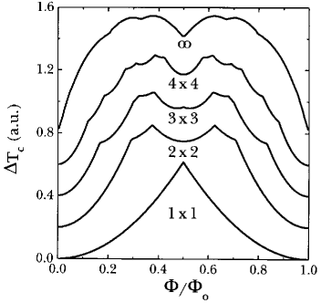
Figure 18: Calculations of the first $T_{c}(H)$ period for an $N\times\,N$ antidot system ($N=1,2,3,4,\infty$) in the London limit.

An important observation is that the amplitude of these ”collective” oscillations depends upon the choice of the resistive criterion. This is similar to the case of Josephson junction arrays and weakly coupled wire networks Giroud92 where phase fluctuations dominate the resistive behavior. The inset of Fig. 17 shows the first collective period, measured using three different criteria. As the criterion is lowered the cusps become sharper and the amplitude increases well above the prediction based on the mean field theory for strongly coupled wire networks Pannetier91 . At the same time, cusps appear at rational fields $\Phi/\Phi_{0}$=1/4, 1/3, 1/2, 2/3 and 3/4 arising from the commensurability of the vortex structure with the underlying lattice.

Above $\sim$ 8 mT, the collective oscillations die out and ”single object” cusps appear, having a periodicity which roughly corresponds to one flux quantum $\Phi_{0}$ per antidot area, $a^{2}$. These cusps are due to the transition between localized superconducting edge states Bezryadin96a having a different angular momentum $L$. These states are formed around the antidots and are described by the same orbital momentum introduced in Section II.C for dots.

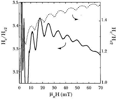
Figure 19: The critical field of Fig. 17 normalized by $\Phi_{0}/2\pi\xi^{2}(T)$ versus the applied field. The dashed line (right axis) shows the theoretical result for a single circular hole with a radius $R=0.24\,\mu m$.

Figure 19 shows the same critical field as shown in Fig. 17, but normalized by the upper critical field $H_{c2}$ of a plain film without antidots, $\mu_{0}H_{c2}=\Phi_{0}/2\pi\xi^{2}(T)$ ( $\xi(0)=36\>\>nm$). The dashed line is the calculation of the reduced critical field for a plain film with a single circular antidot with radius $R=0.24\>\mu m$. The positions of the cusps correspond reasonably well to the experimental ones, taking into account that the model only considers a single hole. From this comparison, an effective area $\pi R^{2}=0.187\>\mu m^{2}$ is determined which is close to the experimental value $a^{2}=0.16\>\mu m^{2}$.

From Figures 17 and 19 it is possible to show that the transition from the network regime to the ”single object” regime takes place at a temperature $T^{*}$ given by the relation $w\approx 1.6\,\xi(T^{*})$, (where $w$ is the width of the superconducting region between two adjacent antidots).

Experiments on systems with other antidot sizes demonstrate that the $a/d$ ratio determines the relative importance of the ”collective regime” and changes the cross-over temperature $T^{*}$. The relation $w\approx 1.6\>\xi(T^{*})$, seems nevertheless to hold reasonably well and is similar to the transition from bulk nucleation of superconductivity to surface nucleation in a thin superconducting slab parallel to the magnetic field Saint-James65 , which happens at a temperature $T_{cr}$ satisfying $w=1.8\>\xi(T_{cr})$.

Comparing the bulk $H_{c2}(T)$ curve with the $T_{c}(H)$ boundary for films with an antidot lattice, we clearly see a qualitative difference between the two, caused by the lateral micro-structuring. In the network limit, $T_{c}(H)$ can be related to the lowest $E_{LLL}$ level in the Hofstadter butterfly Pannetier84 ; Hofstadter76 with pronounced cusps at $n\Phi_{0}$ and the substructure within each period. Reducing the size of the antidot, we are modifying $T_{c}(H)$ substantially but the cusps at $n\Phi_{0}$ are still clearly seen Rosseel97 .

Finally, by introducing antidot lattices we stabilize the novel flux states, which can be briefly characterized as follows. For relatively large antidots sharp cusp-like magnetization anomalies appear at the matching fields $H_{m}$. These anomalies are caused by the formation of the multi-quanta vortex lattices at each subsequent $H_{m}$Baert95a ; Baert95b ; Moshchalkov96 ; Bezryadin96b . The multi-quanta vortex lattices make possible a peaceful coexistence of the flux penetration at the antidots and the presence of a substantial superfluid density in the space between them. This leads to a very strong enhancement of the critical current density in films with an antidot lattice. For smaller antidots the vortices are forced to occupy the interstitial positions after the saturation of the pinning sites at antidotsBezryadin96b ; Rosseel96 ; Harada96 . This leads to the formation of the novel composite flux-line lattices consisting from the interpenetrating sublattices of weakly pinned interstitial single-quantum vortices and multi-quanta vortices strongly pinned by the antidots. When the interstitial flux-line lattice melts, it forms the interstitial flux-liquid coexisting with the flux solid at the antidots.

V Conclusions

We have carried out a systematic study of and quantization phenomena in nanostructured superconductors. The main idea of this study was to vary the boundary conditions for confining the superconducting condensate by taking samples of different topology and, through that, to modify the lowest Landau level $E_{LLL}(H)$ and therefore the critical temperature $T_{c}(H)$. Three different types of samples were used: (i) individual nanostructures (lines, loops, dots), (ii) clusters of nanoscopic elements - 1D clusters of loops and 2D clusters of antidots, and (iii) films with huge regular arrays of antidots (antidot lattices). We have shown that in all these structures, the phase boundary $T_{c}(H)$ changes dramatically when the confinement topology for the superconducting condensate is varied. The induced $T_{c}(H)$ variation is very well decribed by the calculations of $E_{LLL}(H)$ taking into account the imposed boundary conditions. These results convincingly demonstrate that the phase boundaryin $T_{c}(H)$ of nanostructured superconductors differs drastically from that of corresponding bulk materials. Moreover, since, for a known geometry $E_{LLL}(H)$ can be calculated a priori, the superconducting critical parameters, i.e. $T_{c}(H)$, can be controlled by designing a proper confinement geometry. While the optimization of the superconducting critical parameters has been done mostly by looking for different materials, we now have a unique alternative - to improve the superconducting critical parameters of the same material through the optimization of the confinement topology for the superconducting condensate and for the penetrating magnetic flux.

References

- (1) K. Ensslin, and P. M. Petroff, Phys. Rev. B 41, 12307 (1990); H. Fang, R. Zeller, and P. J. Stiles, Appl. Phys. Lett. 55, 1433 (1989); R. Schuster et al., Phys. Rev. B 49, 8510 (1994).
- (2) B. Pannetier, J. Chaussy, R. Rammal, and J. C. Villegier, Phys. Rev. Lett. 53, 1845 (1984).
- (3) M. Tinkham, Phys. Rev. 129, 2413 (1963).
- (4) V. V. Moshchalkov, L. Gielen, C. Strunk, R. Jonckheere, X. Qiu, C. Van Haesendonck, and Y. Bruynseraede, Nature 373, 319 (1995).
- (5) P. G. de Gennes, Superconductivity of Metals and Alloys, Benjamin, New York, 1966.
- (6) J. Romijn, T. M. Klapwijk, M. J. Renne, and J. E. Mooij, Phys. Rev. B 26, 3648 (1982).
- (7) H. Welker, and S. B. Bayer, Akad. Wiss. 14, 115 (1938).
- (8) M. Tinkham, Introduction to Superconductivity, McGraw Hill, New York, 1975.
- (9) W. A. Little, and R. D. Parks, Phys. Rev. Lett. 9, 9 (1962); R. D. Parks, and W. A. Little, Phys. Rev. 133, A97 (1964).
- (10) R. P. Groff, and R. D. Parks, Phys. Rev. 176, 567 (1968).
-
(11)
C. Strunk, V. Bruyndoncx, V. V. Moshchalkov,
C. Van Haesendonck,
Y. Bruynseraede, and R. Jonckheere, Phys. Rev. B 54, R12701 (1996). - (12) P.-G. de Gennes, C. R. Acad. Sci. Ser. II 292, 279 (1981).
- (13) V. V. Moshchalkov, X. G. Qiu, and V. Bruyndoncx, Phys. Rev. B 55, 11793 (1996).
- (14) D. Saint-James, Phys. Lett. 15, 13 (1965); O. Buisson, P. Gandit, R. Rammal, Y. Y. Wang, and B. Pannetier, Phys. Lett. A 150, 36 (1990).
- (15) D. Saint-James, Phys. Lett. 16, 218 (1965).
-
(16)
V. V. Moshchalkov, L. Gielen, M. Baert, V. Metlushko,
G. Neuttiens, C. Strunk, V. Bruyndoncx, X. Qiu, M. Dhallé, K. Temst,
C. Potter,
R. Jonckheere, L. Stockman, M. Van Bael, C. Van Haesendonck, and
Y. Bruynseraede, Physica Scripta T55, 168 (1994). - (17) R. Benoist, and W. Zwerger, Z. Phys. B 103, 377 (1997).
- (18) V. Bruyndoncx, C. Strunk, V. V. Moshchalkov, C. Van Haesendonck, and Y. Bruynseraede Europhys. Lett. 36, 449 (1996).
- (19) S. Alexander, and E. Halevi, J. Phys. (Paris) 44, 805 (1983).
- (20) C. C. Chi, P. Santhanam, and P. E. Blöchl, J. Low Temp. Phys. 88, 163 (1992).
- (21) S. Alexander, Phys. Rev. B 27, 2820 (1983).
- (22) H. J. Fink, A. López, and R. Maynard, Phys. Rev. B 26, 5237 (1982).
- (23) C. Ammann, P. Erdös, and S. B. Haley, Phys. Rev. B 51, 11739 (1995).
- (24) J. I. Castro, and A. López, Phys. Rev. B 52, 7495 (1995).
- (25) R. D. Parks, Science 146, 1429 (1964).
- (26) J. Simonin, D. Rodrigues, and A. López, Phys. Rev. Lett. 49, 944 (1982).
- (27) T. Puig, E. Rosseel, M. Baert, M. J. Van Bael, V. V. Moshchalkov, and Y. Bruynseraede, Appl. Phys. Lett. 70, 3155 (1997).
- (28) B. Pannetier, in Quantum coherence in mesoscopic systems, edited by B. Kramer, (Plenum Press, New York, 1991).
-
(29)
A. Bezryadin, and B. Pannetier,
J. Low Temp. Phys. 98, 251 (1996);
A. Bezryadin et al., Phys. Rev. B 51, 3718 (1995). - (30) M. Giroud et al., J. Low Temp. Phys. 87, 683 (1992); H. S. J. van der Zant, Phys. Rev. B 50, 340 (1994).
- (31) D. R. Hofstadter, Phys. Rev. B 14, 2239 (1976).
- (32) E. Rosseel, T. Puig, M. J. Van Bael, V. V. Moshchalkov, and Y. Bruynseraede, to be published in the proceedings of the conference, Beijing, China, 1997.
-
(33)
M. Baert, V. V. Metlushko, R. Jonckheere,
V. V. Moshchalkov, and
Y. Bruynseraede, Phys. Rev. Lett. 74, 3269 (1995). -
(34)
M. Baert, V. V. Metlushko, R. Jonckheere,
V. V. Moshchalkov, and
Y. Bruynseraede, Europhys. Lett. 29, 157 (1995). - (35) V. V. Moshchalkov, M. Baert, V. V. Metlushko, E. Rosseel, M. J. Van Bael, K. Temst, R. Jonckheere, and Y. Bruynseraede, Phys. Rev. B 54, 7385 (1996).
- (36) A. Bezryadin, and B. Pannetier, J. Low Temp. Phys. 102, 73 (1996).
- (37) E. Rosseel, M. Van Bael, M. Baert, R. Jonckheere, V. V. Moshchalkov, and Y. Bruynseraede, Phys. Rev. B 53, R2983 (1996).
- (38) K. Harada, O. Kamimura, H. Kasai, T. Matsuda, A. Tonomura, and V. V. Moshchalkov, Science 274, 1167 (1996).