Some aspects of electronic topological transition in 2D system on a square lattice. Excitonic ordered states.

Abstract

We study the ordered ”excitonic” states which develop around the quantum critical point (QCP) associated with the electronic topological transition (ETT) in a 2D electron system on a square lattice. We consider the case of hopping beyond nearest neighbors when ETT has an unusual character. We show that the amplitude of the order parameter (OP) and of the gap in the electron spectrum increase with increasing the distance from the QCP, $\delta_{c}-\delta$, where $\delta=1-n$ and $n$ is an electron concentration. Such a behavior is different from the ordinary case when OP and the gap decrease when going away from the point which is a motor for instability. The gap opens at ”hot spots” and extends untill the saddle points (SP) whatever is the doping concentration. The spectrum gets a characteristic flat shape as a result of hybrydization effect in the vicinity of two different SP’s. The shape of the spectrum and the angle dependence of the gap have a striking similarity with the features observed in the normal state of the underdoped high-T_c cuprates. We discuss also details about the phase diagram and the behaviour of the density of states.

Many experiments performed for high $T_{c}$ cuprates provide an evidence for the existence of a pseudogap in the underdoped regime above $T_{c}$ and below some temperature $T^{*}(\delta)$ which value increases with increasing the doping distance from the optimal doping, $\delta_{opt}-\delta$ NMR -Raman . The pseudogap is observed directly by angle-resolved photoemission spectroscopy (ARPES) measurements ARPES -ARPES4 . The striking about this gap is its increase with increasing $\delta_{opt}-\delta$ ARPES2 while the critical temperature of superconducting (SC) transition, $T_{sc}$, decreases. Another prominent feature is the so-called $(\pi,0)$ feature discovered by ARPES: the electron spectrum around the saddle-point (SP) is flat and disappears above some threshold value of wavevector ARPES . Several hypothesis exist about possible origin of the pseudogap KaS -Alt . In this paper we present another explanation of this phenomenon in the framework of the model developed in PRL2 -PRL1 . In these works the concept of the Electronic Topological Transition in 2D system is developed and applied for the explanation of various effects experimentally observed in High - T_c cuprates.

In the present paper we consider various ordered states appearing in the vicinity of ETT point. We show that the ordered ”excitonic” phase On2 formed in a proximity of QCP in a 2D fermion system on a square lattice is characterized (on one side of it, $\delta<\delta_{c}$) by the electron spectrum strikingly similar to that observed in the underdoped cuprates. The mentioned QCP corresponds to the electron concentration $n_{c}=1-\delta_{c}$ at which Fermi level (FL) crosses saddle points (SP) in the bare spectrum. As shown in On2 , in the case of hopping between more than nearest neighbors this point is a point of a fundamental electronic topological transition (ETT) for which singularities in thermodynamical properties (and the logarithmic divergence in density of states at $\omega=0$) is only first quite trivial aspect (related to the local change in topology of the Fermi surface (FS)). The other aspects of criticality related to the mutual change in topology of FS near two different SP’s lead to a very asymmetric behaviour of the noninteracting and interacting system on two sides of ETT being quite anomalous on the side $\delta<\delta_{c}$. On the other hand, for realistic for the high-$T_{c}$ cuprates ratios of hopping parameters $t^{\prime}/t$, $\delta_{c}$ is given by : $\delta_{c}=0.27$ for $t^{\prime}/t=-0.3$ and $\delta_{c}=0.17$ for $t^{\prime}/t=-0.2$, i.e. the anomalous regime $\delta<\delta_{c}$ occurs in the doping range where the experimentally observed ”strange metal” behaviour takes place. Moreover, $\delta=\delta_{c}$ corresponds to a maximum of $T_{sc}(\delta)$ (as discussed in On2 ) and therefore the latter regime can be considered as an underdoped regime.

Some anomalies concerning the ordered ”excitonic” phase have been discussed in PRL2 -PRL3 . Namely, it was shown that the line of the ”excitonic” instability grows from QCP to the side $\delta<\delta_{c}$ instead of having the form of a bell around QCP as it usually happens for an ordinary QCP. Other anomalies which exists in the ordered phase are considered in the present paper. [We call this phase ”excitonic” ordered phase because the discussed instability has the same origin as the classical ”excitonic” instability intensively discussed in the 60-70 KeK -Rice . Namely it is related to the opposite curvature of two parts of electron spectrum in a proximity of FL. In the case considered they correspond to spectra in vicinities of two SP’s.]

We consider various possibilities for the ordered state, namely, Spin and Charge Density Wave orderings with different types of the order parameter symmetries (s-wave, d-wave) depending on the effective interaction between the quasiparticles. Despite of the different symmetries, the properties of such ordered states resemble an ”excitonic” states KeK -Rice are quite similar. The explanation of this phenomenon is in the fundamental role of ETT and effects of criticality in the vicinity of the corresponding QCP PRL1 . We show that the electron spectrum in the ordered phase is characterized by a gap on FL which opens at ”hot spot” and extends until SP whatever is the doping concentration. Therefore there is always a gap at the SP wavevectors $(0,\pm\pi)$, $(\pm\pi,0)$. This remarkable feature is related, as we show in the paper, to a quite nontrivial aspect of ETT: it is the end point of two critical lines for the ”polarization operator” characterizing a behaviour of the free electron system. The other side of the same effect is an increase of the amplitude of the order parameter (and of the gap) with increasing the distance from QCP on the underdoped side. We show also that the electron spectrum in a vicinity of SP gets a specific ”flat” form which on one hand is typical for an ”excitonic” phase (see for example Halp1 ) being a result of a hybridization of two parts of the bare spectrum with the opposite curvature and on the other hand has a striking similarity with the form of the spectrum observed by ARPES ARPES -ARPES4 . We show that the spectrum ”disappears” above some threshold value of wavevector in the direction $(\pi,0)-(\pi,\pi)$ that is also an effect of the same hybridization. We briefly discuss also features related to strong-coupling limit of the model and effects of strong electron correlations.

A starting point is a 2D system of free fermions on a square lattice with hopping between nearest ($t$) and next nearest ($t^{\prime}$) neighbors

$$\epsilon_{{\bf k}}=\ -2t(\cos k_{x}+\cos k_{y})-4t^{\prime}\cos k_{x}\cos k_{y}$$ (1)

(as in On2 we consider $t>0$ and $t^{\prime}<0$) and $|t^{\prime}/t|$ not too small and not too close to the limit $|t^{\prime}/t|=.5$. The dispersion law (1) is characterized by two different saddle points (SP’s) located at $(\pm\ \pi,0)$ and $(0,\pm\pi)$ (in the first Brillouin zone $(-\pi,0)$ is equivalent to $(\pi,0)$ and $(0,-\pi)$ is equivalent to $(0,\pi)$) with the energy $\epsilon_{s}=4t^{\prime}$ . When we vary the chemical potential $\mu$ or the energy distance from the SP, $Z$, determined as

$$Z=\mu-\epsilon_{s}=\epsilon_{F}-4t^{\prime},$$ (2)

the topology of the Fermi surface changes when $Z$ goes from $Z<0$ to $Z>0$ through the critical value $Z=0$, see Fig.1.

In On2 we have shown that such a system undergoes a fundamental ETT at the electron concentration corresponding to $Z=0$. The corresponding quantum critical point is quite rich. It combines several aspects of criticality. The first standard one is related to singularities in thermodynamic properties, in density of states at $\omega=0$ (Van Hove singularity), to additional singularity in the superconducting (SC) response function, all reflect a local change in the topology of FS. This aspect is not important for the properties we are interested in the present paper. Important aspects which reflect a mutual change in the topology of FS in the vicinities of two SP’s are the following. First of all, it is a logarithmic divergence of the polarizalibility of noninteracting electrons

$$\chi^{0}({\bf k},\omega)=\frac{1}{N}\sum_{{\bf q}}\frac{n^{F}(\tilde{\epsilon}_{{\bf q}})-n^{F}(\tilde{\epsilon}_{{\bf{q+k}}})}{\tilde{\epsilon}_{{\bf q+k}}-\tilde{\epsilon}_{{\bf{q}}}-\omega-i0^{+}},$$ (3)

as ${\bf k}={\bf Q}=(\pi,\pi)$, $\omega=0$ and $Z\rightarrow 0$ :

$$\chi^{0}({\bf Q},0)\propto\ln\frac{\omega_{max}}{|Z|}.$$ (4)

which has an ”excitonic” origin ($\omega_{max}\sim t$ is a cutoff energy). By ”excitonic” origin we mean that two branches of the spectrum corresponding to vicinities of two SP’s $(a=t-2t^{\prime},\hskip 8.5359ptb=t+2t^{\prime})$

$$\tilde{\epsilon}_{1}({\bf k})=\epsilon_{1}({\bf k})-\mu=-Z+ak_{x}^{2}-bk_{y}^{2},$$

$$\tilde{\epsilon}_{2}({\bf k})=\epsilon_{2}({\bf k})-\mu=-Z+ak_{y}^{2}-bk_{x}^{2}$$ (5)

have such a form (see Fig.2) that at $Z=0$ the chemical potential lies on the bottom of one ”band” and on the top of the another for the given directions $(0,\pi)-(\pi,\pi)$ and $(\pi,0)-(0,0)$, (see Fig.2). Therefore, no energy is needed to excite the electron-hole pair. It is this divergence that is at the origin of density wave (DW) instability. The DW instability can be of Spin Density Wave (SDW), Charge Density Wave (CDW), Spin Current Density Wave (SCDW) or Orbital Current Density Wave (OCDW) instability Tug ) of interacting electron system depending on a nature of interaction.

The nontriviality stems from the aspect of criticality related to the effect of Kohn singularity in 2D system : the point $Z=0$, $T=0$ is the end of the critical line $Z<0$ each point of which is a point of static Kohn singularities in polarizability of noninteracting electrons. As shown in On2 , the latter aspect is a motor for the anomalous behaviour of the system on the side $Z>0$ of ETT. One among the anomalies found in On2 concerns the ordered DW phases. We have obtained that the line of DW ”excitonic” instability $T_{DW}(Z)$ has the anomalous form on the side $Z>0$ : it grows from QCP instead of having the form of a bell around QCP as it usually happens in the case of ordinary QCP and as it indeed happens on the side $Z<0$. Below we show that this latter aspect is also at the origin of anomalous behaviour of the order parameter and of some other anomalies in the ordered state in the same regime $Z>0$.

As shown in On2 , on the side $Z>0$ of the electronic topological transition, a maximum of the static electron-hole susceptibility occurs at the wavevector ${\bf q=Q}$. Therefore in a presence of $\bf q$ independent interaction or $\bf q$ dependent interaction negative for ${\bf q=Q}$, the DW instability happens at ${\bf q=Q}$ and this is the wavevector of ordering in the DW phase. As usual for such phases, one should consider a matrix electron Green function containing as components the normal and anomalous Green functions in terms of operators $a^{+}_{{\bf k},\sigma}$ and $a_{{\bf k}\sigma}$ which are the creation and annihilation electron’s operators respectively:

$$K_{11}({\bf k},i\omega_{n})=-\int_{0}^{\beta}d\tau e^{i\omega_{n}\tau}<T_{\tau}a_{{\bf k}\sigma}(\tau)|a^{+}_{{\bf k}\sigma}(0)>$$

$$K_{22}({\bf k},i\omega_{n})=-\int_{0}^{\beta}d\tau e^{i\omega_{n}\tau}<T_{\tau}a_{{\bf k+Q}\sigma}(\tau)|a^{+}_{{\bf k+Q}\sigma}(0)>$$

$$K_{12}^{\sigma\sigma^{\prime}}({\bf k},i\omega_{n})=-\int_{0}^{\beta}d\tau e^{i\omega_{n}\tau}<T_{\tau}a_{{\bf k+Q}\sigma}(\tau)|a^{+}_{{\bf k}\sigma^{\prime}}(0)>.$$ (6)

[Below we will omit spin indices in the Green functions keeping in mind that $K_{12}=K_{12}^{\sigma-\sigma}$ for CDW and OCDW states and $K_{12}=K_{12}^{\sigma\sigma}$ for SDW and SCDW states.]

If the anomalous Green function $K_{12}$ is nonzero (that should be found selfconsistently) the explicit expressions for the two Green functions are as follows

$$K_{11}({\bf k},i\omega_{n})=\left[\frac{u^{2}({\bf k})}{i\omega_{n}-\varepsilon_{1}}+\frac{v^{2}({\bf k})}{i\omega_{n}-\varepsilon_{2}}\right]$$

$$K_{22}({\bf k},i\omega_{n})=\left[\frac{u^{2}({\bf k})}{i\omega_{n}-\varepsilon_{2}}+\frac{v^{2}({\bf k})}{i\omega_{n}-\varepsilon_{1}},\right]$$

$$K_{12}({\bf k},i\omega_{n})=K_{21}({\bf k},i\omega_{n})=$$

$$=u({\bf k})v({\bf k})\left[\frac{1}{i\omega_{n}-\varepsilon_{1}}-\frac{1}{i\omega_{n}-\varepsilon_{2}}\right],$$ (7)

where $u$, $v$ - coefficients have a standard form :

$$u^{2}({\bf k})=\frac{1}{2}\left[1+\frac{\epsilon_{A}(k)-\epsilon_{B}(k)}{2E({\bf k})}\right],$$

$$v^{2}({\bf k})=\frac{1}{2}\left[1-\frac{\epsilon_{A}(k)-\epsilon_{B}(k)}{2E({\bf k})}\right],$$

$$E({\bf k})=\sqrt{\left(\frac{\epsilon_{A}-\epsilon_{B}}{2}\right)^{2}+|\Delta({\bf k})|^{2}}.$$ (8)

The spectrum in the ordered state is given by

$$\varepsilon_{1,2}=\frac{\epsilon_{A}+\epsilon_{B}}{2}\pm\sqrt{\left(\frac{\epsilon_{A}-\epsilon_{B}}{2}\right)^{2}+|\Delta({\bf k})|^{2}},\;\;\;\;\;\;\;$$

$$\epsilon_{A}({\bf k})\equiv\epsilon({\bf k})\;\;\;\;\;\;\;\;\epsilon_{B}({\bf k})=\epsilon({\bf k+Q}),$$ (9)

where $\epsilon({\bf k})$ is defined by (1). The equation for the gap is

$$\Delta({\bf k})=-T\sum_{\omega_{n}}\frac{1}{N}\sum_{\bf p}\Gamma_{12}({\bf k,k+Q,p})K_{12}({\bf p},i\omega_{n})$$ (10)

where $\Gamma_{12}$ is a vertex which in mean field approximation coincides with the bare interaction:

$$\Gamma_{12}({\bf k,k+Q,p})=V_{\bf Q},\;\;\;for\;SDW\;\;(CDW)$$

$$\Gamma_{12}({\bf k,k+Q,p})=V_{\bf k-p},\;for\;OCDW\;\;(SCDW)$$ (11)

where $V_{\bf k}=2V(\cos(k_{x})+\cos(k_{y}))$. The type of the interaction and therefore, type of the excitonic phase depend on the model. The SDW and OCDW instabilities occur in the case of a positive interaction in the triplet channel (exchange interaction), the CDW and SCDW instabilities take place for positive interaction in the singlet channel (density-density interaction). We will not fix for the moment a type of interaction and therefore a nature of the ordered phase assuming that there exists either the first or the second interaction.

The equation (10) is reduced to the following equation

$$1=4|V|\Pi^{DW}_{\bf k=0}({\bf Q},Z,\Delta)$$ (12)

where the ”polarization operators” $\Pi^{DW}({\bf Q},Z,\Delta)$ are given by one of the following equations DW :

$$\Pi^{SDW,CDW}({\bf Q},Z,\Delta)=$$

$$=\frac{1}{4N}\sum_{p}\frac{1}{E({\bf p})}[\tanh(\frac{\varepsilon_{1}}{2T})-\tanh(\frac{\varepsilon_{2}}{2T})],$$ (13)

$$\Pi^{OCDW,SCDW}({\bf Q},Z,\Delta)=$$

$$=\frac{1}{4N}\sum_{p}\frac{(\cos p_{x}-\cos p_{y})^{2}}{4E({\bf p})}[\tanh(\frac{\varepsilon_{1}}{2T})-\tanh(\frac{\varepsilon_{2}}{2T})]$$ (14)

The expressions (12) are the equation for the SDW, CDW, OCDW or SCDW gap which should be solved selfconsistently. We emphasis that for $V>0$ only SDW (OCDW) solution is possible whereas CDW (SCDW) solution takes place for $V<0$.

The solution of (12)-(14) is given by one of the following expressions

$$\Delta=\Delta^{SDW}({\bf k})=\Delta^{SDW}_{0},$$

$$\Delta=\Delta^{CDW}({\bf k})=\Delta^{CDW}_{0},$$

$$\Delta=\Delta^{OCDW}({\bf k})=\Delta^{OCDW}_{0}(\cos k_{x}-\cos k_{y})/2,$$

$$\Delta=\Delta^{SCDW}({\bf k})=\Delta^{SCDW}_{0}(\cos k_{x}-\cos k_{y})/2$$ (15)

The equations (10)-(15) are quite standard. A nontriviality, as we show below, is related to the behaviour of the ”polarization operator” in a proximity of ETT. As we have shown in On2 , the effect that the point of ETT is the end point of the critical line $Z<0$ leads to the anomalous behaviour of the electron-hole susceptibility $\chi^{0}({\bf Q},Z,\omega)$ on the side $Z>0$. Below we show that a similar effect takes place for the ”polarization operator” (14). The two functions coincides in the limit cases: $\chi^{0}({\bf Q},Z,\omega=0)=\Pi^{DW}({\bf Q},Z,\Delta=0)$. [It is important to emphasize that the behaviour of the ”polarization operator” depends only on properties of the system of noninteracting electrons, namely on the topology of FS.]

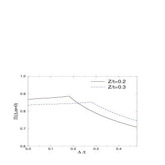
Figure 3: Calculated ”polarization operator” $\Pi({\bf Q},Z,\Delta(Q))$ as a function of $\Delta_{0}$ for fixed $Z$ and $T=0$.

Calculated for $T=0$ ”polarization operators” $\Pi^{DW}$
$({\bf Q},Z,\Delta_{0})$ as a function of $\Delta_{0}$ for fixed $Z$ (in the regime $Z>0$) are shown in Fig.3. Since the properties of the ”polarization operators” are similar in many aspects we shall omit later the indices (SDW, CDW, OCDW or SCDW) except for the cases when it will be necessary to emphasize the difference.

One can see that there is a singularity at some point $\Delta_{0}=\Delta_{c}(Z)$. The value of $\Delta_{c}(Z)$ increases with increasing $Z$. The situation is quite similar to that analyzed in On2 for $\chi^{0}$ as a function of $\omega$ for fixed $Z$ and $T=0$. In the latter case we have found a square-root singularity at

$$\omega=\omega_{c}=\frac{2Z}{1-2t^{\prime}/t},$$

which is the dynamic Kohn singularity. As we see in Fig.3, for the polarization operator $\Pi({\bf Q},Z,\Delta)$ the singularity is weaker, while $\Delta_{c}(Z)$ also scales with $Z$.

Analytical estimations show that $\Delta_{c}(Z)$ is given by

$$\Delta_{c}(Z)=Z$$ (16)

while the asymptotic form of $\Pi(Q,Z,\Delta)$ near the singularity is given by :

$$t\Pi(Q,Z,\Delta)=\left\{\begin{array}[]{cc}\displaystyle A_{1}|1-\Delta/\Delta_{c}|+B,&\hskip 8.5359pt\Delta<\Delta_{c}\\ \displaystyle A_{2}|1-\Delta/\Delta_{c}|+B,&\hskip 8.5359pt\Delta>\Delta_{c}.\end{array}\right.$$ (17)

The jump in the derivative, $A_{1}-A_{2}$, depends only on $t^{\prime}/t$ const and is proportional to

$$A_{1}-A_{2}\propto\frac{1}{|t^{\prime}/t|}\left(\ln|\frac{4}{t^{\prime}/t}|-A_{0}\right),$$ (18)

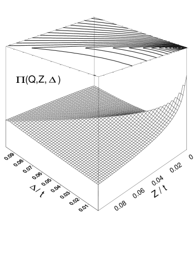
Figure 4: $\Pi({\bf Q},Z,\Delta_{0})$ as a function of $\Delta_{0}$ and $Z$ at $T=0$ and lines $\Pi^{zz}({\bf Q})=const$ in $Z-\Delta_{0}$ coordinates.

where $A_{0}$ is a constant (for the spectrum (5) $A_{0}=\pi/8$). The critical line (16) is clearly seen in Fig.4a where we present the calculated $\Pi({\bf Q},Z,\Delta_{0})$ as a function of $Z$ and $\Delta_{0}$. From the point of view of the behaviour of the ”polarization operator”, the ETT point is the end point of two critical lines. The first is the semiaxis $Z<0$ each point of which corresponds to the square-root singularity in $\Pi({\bf q},Z,\Delta)$ occurring as $\Delta_{0}\rightarrow 0$ and ${\bf q}\rightarrow{\bf q}_{m}$, where the latter is the characteristic for this regime wavevector of incommensurability (see On2 where the ${\bf q}$ dependence of $\Pi({\bf q},Z,0)$= $\chi^{0}({\bf q},Z)$ is analyzed in details.) The second is the line $Z=\Delta_{0}$ each point of which corresponds to the kink in $\Pi({\bf q},Z,\Delta(q))$ occurring at $T=0$ as ${\bf q}\rightarrow{\bf Q}$ where the latter is the characteristic wavevector for the regime $Z>0$. At the point of intersection of these lines, $Z=0$, the two types of singularities are transforming into the logarithmic singularity ; $\Pi({\bf q},0,\Delta)\propto\ln|\max({\bf q-Q},\Delta)|$.

The existence of the growing with $Z$ critical line determines a quite unusual form of the lines $\Pi(Q,Z,\Delta)=constant$ which develop around the critical line $\Delta_{c}(Z)$ and grow with increasing $Z$, (see Fig.4(b)).

In preceeding discussion we presented some general analysis which does not depend on details of interaction considered but only on the topology of the FS. To provide the calculations, let us consider a particular case of interaction resulting in Spin Density Wave (11),(13). The solution of corresponding eq. (12) for $t/V=1.8$ is shown in Fig.5. Two branches of the solution have an anomalous dependence of the gap on $Z$ reproducing the form of the lines $\Pi(Q,Z,\Delta_{0})=constant$ in Fig.4(b). The anomaly is that for both solutions gap increases with increasing the distance from the quantum critical point, i.e. from the point which is at the origin of the ordered phase. [For an ordinary QCP the gap is maximum at the electron concentration corresponding to QCP and decreases monotonously with increasing the distance from QCP. For example such a picture takes place for DW phase on both sides from QCP in the case of $t^{\prime}=t^{\prime\prime}=...=0$; as we discussed in On2 in the latter case all anomalies in the regime $\delta<\delta_{c}$ disappear. In the case considered in the paper it happens on the overdoped side of the QCP.]

The difference between two solutions for the gap presented in Fig.5 is that

$$\Delta_{1}(Z)>Z$$ (19)

while

$$\Delta_{2}(Z)<Z$$ (20)

for any $Z$, any $t/V$, any $t^{\prime}/t$ since the two lines, $\Delta_{1}(Z)$ and $\Delta_{2}(Z)$ are attached to the critical line $\Delta=\Delta_{c}(Z)=Z$ from above and from below. For the most range of the existence of the ordered phase $Z<Z_{cr}^{(1)}$, see Fig.5, only one solution exists, the one corresponding to eq. (12). In the hyperbolic approximation and under the condition $|t^{\prime}/t|$ not too small $Z_{cr}^{(1)}$ is given by:

$$Z_{cr}^{(1)}\propto\omega_{max}\exp(-\pi^{2}t/(V\ln|t/t^{\prime}|)).$$

For this solution one has

$$\Delta_{1}(Z)\equiv\Delta_{0}(Z)=f(Z)+\Delta(0)$$ (21)

where $\Delta(0)$ is given by

$$\Delta(0)\propto|t^{\prime}|\exp(-\frac{2\pi^{2}|t^{\prime}/V|}{\sqrt{1-(2t^{\prime}/t)^{2}}}),$$ (22)

and $f(Z)$ is an increasing function of $Z$, linear under the condition $\Delta(Z)\gg\Delta(0)$. The expression (22) is valid under condition $\pi^{2}|t^{\prime}/V|/\sqrt{1-(2t^{\prime}/t)^{2}}\gg 1$. For the narrow $Z$ range of the coexistence of the two solutions $Z_{cr}^{(1)}<Z<Z_{cr}^{(2)}$ it is the solution $\Delta_{1}$ which is favorable (see Appendix). Therefore, the value of the gap increases with increasing $Z$ being always larger than $Z$. As we have shown, this is a consequence of the effect that the point of ETT is the end point of two critical lines.

Let’s analyze now the form of the spectrum in the DW phase. The spectrum given by (9) is plotted in Fig.6. for three important directions : $(\pi,\pi)-(\pi,0)-(0,0)$ and $(0,0)-(\pi,\pi)$. The spectrum in the vicinity of SP has the following prominent features: The first is a characteristic ”flat” shape (very close to the experimental shape ARPES , see Fig.8(a) being a consequence of the hybridization of the two branches of the bare spectrum in the vicinity of two different SP’s with the opposite curvatures, (see Fig.7).

The second: the spectrum in the direction $(\pi,\pi)-(0,\pi)$ ”disappears” above some threshold value of wavevector since the residue $v^{2}_{\bf k}$ tends to zero (that is also an ordinary consequence of the hybridization). On the other hand, since

$$\varepsilon_{1}({\bf k}_{SP})=-Z+\Delta,$$

$$\varepsilon_{2}({\bf k}_{SP})=-Z-\Delta$$

(see, e.g. Eq.(9)) and $\Delta>Z$, the chemical potential always lies in the gap for the part of Brillouin zone (BZ) starting from the ”hot spot” until SP that is a consequence of the existence of the critical line $\Delta=\Delta_{c}$ related to the discussed above aspect of criticality of the QCP. For the direction $(0,0)-(1,1)$, Fermi level lies in the lower branch of the spectrum, (see Fig.6(b)), i.e. the system remains metallic. The theoretical spectrum has a striking similarity with the anomalous experimental electron spectrum in the underdoped cuprates observed below the characteristic line $T^{*}(\delta)$ by ARPES ARPES , we reproduce it in Fig.8. We remind that ARPES measures a spectral function only below FL.

Then in Fig.9 we present the angle dependence of the value of $\epsilon_{\bf k}-\mu$, i.e. of the gap calculated from FL, in the same way as it is done in ARPES experiments ARPES0 . Namely we plot the minimal value of $|\varepsilon_{\bf k}-\mu|$ for each given direction. The dependence is of a ”d-wave type” in a sense that the gap increases with increasing the argument $(\cos k_{x}-\cos k_{y})$ almost linearly in the proximity of SP. However the dependence is flat (not linear as it happens in the d-wave case) when approaching the direction $(1,1)$. Such a behaviour is also close to the experimentally found behaviour above $T_{c}$ ARPES0 reproduced in Fig.9(b). [Although the authors of ARPES0 claim that the behaviour observed above and below $T_{c}$ is the same, what one sees in the experimental plot is not exactly this : the behaviour above and below $T_{c}$ is similar in the vicinity of SP and different when approaching the $(1,1)$ direction and this occurs quite systematically, see also the plots in ARPES0 for other samples.]

We considered the particular case of SDW as an example of ordreed ”excitonic” state. Nevertheless, all aforesaid is true for any other types of ordered states since the existence of such states is determined only by topology of FS.

Let us study now the one particle density of states (DOS) given by the expression

$${\cal N}(\varepsilon)=-\frac{1}{\pi}\frac{1}{N}\sum_{\bf p}[{\it Im}K_{11}^{R}({\bf p},\varepsilon)+{\it Im}K_{22}^{R}({\bf p},\varepsilon)]=$$

$$=\frac{1}{N}\sum_{\bf p}[\delta(\varepsilon-\varepsilon_{1}({\bf p}))+\delta(\varepsilon-\varepsilon_{2}({\bf p}))],$$ (23)

Numerical calculations with the spectrum (1) give the picture shown in Fig.10.

The density of states of SDW (CDW) states deviates from the DOS in the initial metallic state in two $\varepsilon$ ranges notated as A and B. For OCDW (SCDW) states only feature A survives. Analytical calculations show that the A-feature is related to the existence of the discussed above QCP (which we call below QCP1). Calculations of the integral in (23) performing with the hyperbolic spectrum (5) valid in the vicinities of SP’s show that in the A range DOS is characterized by three singularities (instead of one logarithmic singularity in the bare density of states ${\cal N}_{0}(\varepsilon)$ as $\varepsilon\to-Z$). Those are a logarithmic singularity at $\varepsilon_{1}=-Z-\Delta_{0}\sqrt{1-4(t^{\prime}/t)^{2}}$ Arist

$${\cal N}(\varepsilon\to\varepsilon_{1})\sim\frac{1}{t\sqrt{1-4(t^{\prime}/t)^{2}}}\ln(\frac{\omega_{max}}{|\varepsilon-\varepsilon_{1}|})$$ (24)

and jumps at two energies

$$\varepsilon_{2,3}=-Z\pm\Delta_{0}.$$

The distance between two jumps is equal to $2\Delta$.

The B feature is related to the existence of the second quantum critical point in the system (QCP2) discussed in On3 . This point corresponds to the electron concentration when the chemical potential is equal : $\mu=\mu_{c2}=0$ or by other words when the wavevector connecting two parts of FS in the direction $(1,1)$ is equal to ${\bf Q}_{AF}=(\pi,\pi)$. In this case two ”hot spots” on FS come together at the singular position $(\pm\pi/2,\pm\pi/2)$ before disappearing. The calculations of the integral in (23) with the spectrum taken around $(\pi/2,\pi/2)$ give a logarithmic divergence at the point $\varepsilon_{4}=-Z-4t^{\prime}+\Delta(\pi/2,\pi/2)$:

$${\cal N}(\varepsilon\to\varepsilon_{4})-{\cal N}_{0}(\varepsilon_{4})\sim\frac{1}{t}\sqrt{\frac{\Delta(\pi/2,\pi/2)}{|t^{\prime}|}}\ln(\frac{\omega_{max}}{|\varepsilon-\varepsilon_{4}|})$$ (25)

and a jump at the point $\varepsilon=-Z-4t^{\prime}-\Delta(\pi/2,\pi/2)$. This feature does not exist for OCDW (SCDW) states since $\Delta({\bf k})=0$ along the diagonal of BZ.

The B feature is important in the case when the chemical potential lies close to the pseudogap in the B part that should take place in the electron-doped cuprates. For the hole-doped cuprates we are interested in the present paper, it is QCP1 which determines properties of the system. In this case the chemical potential lies in the ”pseudo-gap” A according to the properties of the electron spectrum in the vicinity of SP discussed above.

Let’s analyze now the range of the existence of the ordered phase in the $T-Z$ plane. For this sake let’s analyze the behaviour of $\Pi({\bf Q},Z,\Delta_{0})$ as a function of $Z$ at finite temperature. [We again consider SDW state for certainity.] Results of calculations are presented in Fig.11. The first observation is that the gap changes only little with $T$ at low $T$. The second is that the behaviour at finite temperature as a function of $Z$ is qualitatively the same as for $T=0$ and it is anomalous: the value of the gap increases with increasing $Z$.

The phase diagram in $T-Z$ plane obtained for SDW (CDW) instability based on the analysis of the gap behaviour at finite $T$ is presented in Fig.12. It is worthwhile to note that the polarization operator $\Pi$ $({\bf Q},Z,\Delta)$ (14) calculated for OCDW (SCDW) ordered states has essentially more abrupt behavior as a function of $Z$ in comparison with those for $\Pi^{SDW,CDW}$$({\bf Q},Z\Delta)$ (13). Such behaiour appears due to additional factor $(\cos(p_{x})-\cos(p_{y}))^{2}$ in the integral (12). As a result, the domain of existence of OCDW (SCDW) solutions for equation (12) at various doping concentrations is substantially narrower than for SDW (CDW) case. Nevertheless, it does not affect on the qualitative shape of phase diagram Fig.12.

The solid line is the line where $\Delta_{1}(T)=0$. The dashed line is the line where $\Delta_{2}(T)=0$. These two lines are at the same time the lines of instabilities of the undistorted metallic state. The line $\Delta_{2}(T)=0$ is not however a line of a phase transition since the nonzero solutions for the gap exist on the left of this line until the dot-dashed line. Along the latter line corresponding to the disappearance of the ”ordered” solution, the gap is finite and the two solutions coincide : $\Delta_{0}(T)=\Delta_{1}(T)=\Delta_{2}(T)$. The situation is clearly seen from Fig.13 where we present the lines $\Pi({\bf Q},Z,\Delta)=const$ for different $Z$ and fixed $t/J$ which in fact give the full picture of the behaviour of the DW gap as a function of $Z$ and $T$.

As we discuss in the Appendix, in the region between the dot-dashed and dashed line, where three solutions $\Delta_{0}=\Delta_{1}$, $\Delta_{0}=\Delta_{2}$ and $\Delta=0$ coexist, it is the solution $\Delta_{0}=\Delta_{1}$ which is energetically favorable.

Thus, the dot-dashed line in the phase diagram in Fig.12 is the line of the first-order phase transition. The gap along this line changes only little at low temperature and tends to zero rapidly in the vicinity of the point $O$. The latter is a tricritical point. The range in $T-Z$ plane in the vicinity of this point corresponds to a strongly fluctuating regime which we will consider elsewhere. It is important to add also that at the point $Z=Z_{cr}^{(2)}$ of the appearance of the ordered phase at $T=0$, the gap is exactly equal to $Z$ that means that the upper branch of the spectrum in Fig.6(a) touches FL. Then when moving inside the ordered phase the gap $\Delta$ becomes larger than $Z$ and this branch goes up leaving the FL.

Above we have considered the critical temperatures and the gap behaviour as functions of the energy distance from the QCP, $Z$. It is worth for applications to cuprates to change the description and to consider physical properties as functions of electron concentration $n_{e}$ or of hole doping $\delta=1-n_{e}$. To do this we use the relation between $Z$ (or the chemical potential $\mu$) and the hole doping which for $T=0$ is given by :

$$1-\delta=\int_{\omega}N(\omega)d\omega.$$ (26)

So far as

$$Z\propto\delta_{c}-\delta,$$ (27)

all dependencies considered above can be rewritten as functions of doping distance from QCP. For example, the phase diagram in the plane $T-\delta$ calculated for $t^{\prime}/t=-0.3$ for which $\delta_{c}=0.27$ gets the form shown in Fig.14.

One can easily obtain values of doping for all plots presented in Fig.4-Fig.11 when comparing the phase diagram in $T-Z$ plane in Fig.12, and in $T-\delta$ plane in Fig.14.

Obviously, the gap $\Delta_{0}(\delta)$ increases with $\delta_{c}-\delta$ in the same way as it increases with $Z$, see Fig.5 and Fig.11 for $\Delta_{0}=\Delta_{1}$.

All features discussed above do not depend on the nature of the ordered phase, SDW, CDW, OCDW or SCDW since they reflect the topological aspects of ETT. The type of the excitopic phases developing around ETT point depend on the type of interaction. It is the SDW or OCDW state in the case of a positive interaction in the triplet channel (exchange interaction) and the CDW or SCDW state in the case of a positive interaction in a singlet channel (density-density interaction). The ordered SDW phase is characterized by spin ordering with momentum $<S^{z}_{Q}>=1/2(<n_{\sigma\sigma}(Q)>-<n_{\bar{\sigma}\bar{\sigma}}(Q)>)=\Delta_{0}$ and the CDW phase by the charge ordering. In the SCDW (OCDW) the staggered magnetization (density) is equal to zero. Nevertheless, the spin-current (charge-current) correlation functions survive.

In our opinion for the case of high-$T_{c}$ cuprates it is the interaction in the triplet channel which determines the behaviour of the system and the nature of DW phase. From the theoretical point of view it is this situation which corresponds to the strong-coupling limit models : the Hubbard model and the $t-J$ model. For example for the latter with the $J$ term written as $H_{J}=\sum_{ij}J_{ij}\{a\vec{S}_{i}\vec{S}_{j}-(b/4)n_{i}n_{j}\}$ one has $V^{SDW}_{\bf q}=aJ_{\bf q}$ while $V^{CDW}_{\bf q}=-\frac{b}{4}J_{\bf q}$, i.e. the interaction in the triplet channel is positive while in the singlet channel is negative. This version is supported also by experiments in the high-$T_{c}$ cuprates : observed experimentally (by INS, see for example Rossat-Mignod and NMR) strong magnetic response around ${\bf q}={\bf Q}$ is a phenomenological argument in a favor of a strong momentum dependent interaction in a triplet channel, i.e. of $V_{\bf q}=J_{\bf q}$ ($J>0$). However, we can not exclude an importance of an interaction leading to the CDW (SCDW) order.

Another point concerning the interaction is its strength. Depending on the ratio $|V|/W$ (where $W$ is an energy bandwidth), maximal $T_{DW}^{max}$ can be high or low. Respectively, the DW phase can lean out of SC state or can be hidden under it. [In the presence of the interaction in the triplet channel, $J_{\bf q}$, both SDW and SC instabilities occur around QCP1 under the same condition : $J>0$, for the SC instability see On1 ]. It is temptating to identify the properties obtained for the DW state with the properties observed experimentally in the underdoped cuprates above $T_{sc}(\delta)$ and below $T^{*}(\delta)$. Indeed they have a striking resemblance, as one can see when comparing Fig.6 and Fig.8, Fig.9(a) and Fig.9(b) and when comparing the behaviour of the gap as a function of $Z$ (or doping, $\delta_{c}-\delta$) with the experimental behaviour ARPES2 . Our calculations (when considering both d-wave SC and DW instabilities in the presence of interaction $J$ in the triplet channel) show that the answer is quite subtle. When $t^{\prime}/t=-0.2$ the ordered DW phase leans out of the SC phase for $t/J<1.90$, for $t^{\prime}/t=-0.3$ this happens when $t/J<1.55$. So far as realistic value of $t/J$ for cuprates is estimated to be in the interval $t/J=1-3$, both variants (when the DW phase leans out or is hidden under the SC phase) are possible.

In this case two scenarios can be discussed. First, the DW state of s- or d- wave symmetry can coexist with d-wave SC state (this situation is considered in Bouis ) resulting in appearance of supplementary $\pi$-triplet state. Second, the DW state can be suppressed under the SC state. Nevertheless, the strong ”fluctuation” memory of this ordering will affect on the behaviour of disordered metallic state.

Even in the case if the long-range ordered DW phase is hidden under SC phase it is this type of ordering which determines short range correlations in the disordered metallic state above $T_{c}$ and below $T^{*}(\delta)$. This point is discussed in On2 ,PRL2 . The state below $T^{*}(\delta)\propto\delta_{c}-\delta$ and above $T_{c}$ is quite exotic. It is almost frozen in both temperature and doping. By this we mean that the parameter $\kappa^{2}$ which determines a proximity to the ordered DW phase does almost not change neither with $T$ nor with doping remaining therefore quite low in a wide region in $T-\delta$ plane below $T^{*}(\delta)$. Such a quasiordered state keeps a strong memory about the ordered phase. Therefore, electron properties in this state should be close to those in the DW ordered state being however characterized by strong damping. [By the way it is exactly what is observed by ARPES. The experimental electron spectrum has a form shown in Fig.8. being however characterized by a spectral function of a very damped form. Explicit consideration of the electron spectrum in this state will be presented elsewhere].

Summarizing, we have studied the DW phase which is formed around QCP1 (associated with ETT) and we have shown that this phase is characterized by the following prominent features:

(i) the specific ”flat” shape of the spectrum in the vicinity of SP,

(ii) ”disappearance” of the spectrum above some threshold value of wavevector in the direction $(\pi,0)$ - $(\pi,\pi)$,

(iii) pseudogap in DOS with FL lying in it,

(iv) increasing of the gap in the spectrum around SP and of the pseudogap in DOS with decreasing doping for $\delta_{c}-\delta$

(v) angle dependence of the gap calculating from FL which is of a d-wave type close to SP and flat close to the direction $(1,1)$.

All these features have a striking similarity with the experimental features revealed by ARPES in the normal state of the underdoped hole-doped cuprates.

Appendix A

The free energy density in the approximation corresponding to considered in the paper is given by:

$$F=-T\frac{1}{N}\sum_{\bf k}\sum_{\alpha=1,2}[\ln(2\cosh(\frac{\varepsilon_{\alpha}({\bf k},\Delta_{\bf k})}{2T}))+\frac{\Delta_{\bf k}^{2}}{4}]+\mu n.$$ (28)

[Note that the equation (10) corresponds to $\partial F/\partial\Delta=0$.] Therefore, the difference between free energies corresponding to $\Delta=\Delta_{1}$ and $\Delta=\Delta_{2}$ is given by

$$F_{1}-F_{2}=\frac{\Delta_{1}^{2}-\Delta_{2}^{2}}{4V}-T\frac{1}{N}\sum_{\bf k}\sum_{\alpha=1,2}\ln\left(\frac{\displaystyle\cosh(\frac{\varepsilon_{\alpha}({\bf k},\Delta_{1})}{2T})}{\cosh(\frac{\displaystyle\varepsilon_{\alpha}({\bf k},\Delta_{2})}{2T})}\right).$$ (29)

One can check by numerical calculations that $F_{1}-F_{2}<0$ for the whole range of the coexistence of the two solutions.

Some analytical estimations can be also done for low $T$ based on the well-known expression AGD for the difference between thermodynamic potentials of the ordered and disordered states:

$$\delta\Omega=\Omega(\Delta_{1})-\Omega(0)=\int_{0}^{\Delta_{1}}\frac{d(1/V)}{d\Delta}\Delta^{2}d\Delta.$$ (30)

When substituting the expressions for $\Delta_{1}$ (21), (22) one gets

$$\delta F/t=\delta\Omega/t\sim-\frac{\sqrt{1-4|t^{\prime}/t|^{2}}}{|t^{\prime}/t|}\frac{\Delta_{1}^{3}}{t^{2}\Delta(Z=0)}\sim-\frac{(Z_{cr}^{(1)})^{3}}{t^{2}\Delta(Z=0)}.$$ (31)

One can see that this correction is negative. Therefore, the solution $\Delta=\Delta_{1}$ is favorable with respect to the solution $\Delta=0$ for any $Z_{cr}^{(1)}<Z<Z_{cr}^{(2)}$.

^∗ Present address: Institüt für Theoretische Physik, Universität Würzburg, D-97074 Würzburg, Germany

Figure 1: Fermi surface of the electron system with the dispersion law (1) for different Z and $t^{\prime}/t=-0.3$. The thick line corresponds to $Z=0$.

Figure 2: Schematic presentation of the electron spectrum in a vicinity of two SP’s for $Z=0$

Figure 5: Gap $\Delta$ obtained by solving equations (12), (14) as function of Z (t/V=1.8, $t^{\prime}/t=-0.3$). The solid line corresponds to $\Delta_{1}(Z)$, the dot-dashed line to $\Delta_{2}(Z)$, the dashed line to $\Delta_{c}(Z)$.

a)                                                    b)

Figure 6: One particle spectra along $(\pi,\pi)-(\pi,q_{y}/\pi)$ and $(\pi-q_{x}/\pi,0)-(0,0)$ symmetry lines (a) and in $(0,0)$ -$(\pi,\pi)$ direction (b), $t^{\prime}/t=-0.3,t/V=1.8,Z/t=0.03$. Long dashed line is the bare spectrum, dot-dashed line corresponds to the spectrum when the residue of the Green function (7) less than 0.1.

Figure 7: Schematic representation of the bare spectrum in the vicinity of the two saddle points for $Z\neq 0$.

a)                                                    b)

Figure 8: Experimental one particle spectra along $(\pi,\pi)-(\pi,0)-(0,0)$ symmetry lines (a) and in $(0,0)$ -$(\pi,\pi)$ direction (b) measured in the overdoped regime of BSCO. The data are taken from [10].

a)                                   b)

Figure 9: Theoretical angle dependence of the SDW gap calculated from FL in the underdoped regime $Z>0$ ($t^{\prime}/t=-0.3$, $t/V=1.7$, $Z/t=0.3$) (a) and the experimental leading edge midpoint measured by ARPES in the underdoped BSCO [11] (b).

Figure 10: Density of states in the ordered ”excitonic” phase calculated for $Z/t=0.03$ ($t/V=1.8,t^{\prime}/t=-0.3$). Dashed line corresponds to the DOS in the initial metallic state.

Figure 11: The DW gap in $t$ units as a function of $Z$ for increasing temperature : $T/t=0.005,0.1,0.2$ ($t^{\prime}/t=-0.3$, $t/V=1.8$).

Figure 12: Phase diagram around QCP1 in T-Z coordinates ($t/V=1.8$, $t^{\prime}/t=-0.3$). We show only the regime $Z>0$ corresponding to the anomalous behavior. The solid line is a line of second-order phase transition, the dot-dashed is a line of first-order phase transition and the dashed line is a line of instability of the disordered metal state (spinodal). The point $O$ is a tricritical point.

a)                                                    b)

Figure 13: Lines of $\Pi({\bf Q},Z,\Delta)=const$ for fixed $t/V=1.8$ and different $Z$. The plot (b) is a zoom of the plot (a) corresponding to the coexistence of the two solutions for the gap.

Figure 14: Phase diagram around QCP1 in T-$\delta$ coordinates ($t/V=1.8$, $t^{\prime}/t=-0.3$)

References

- (1) H. Alloul, T. Ohno, P. Mendels, Bull. Am. Phys. Soc. 34, 633 (1989), H. Alloul, T. Ohno, P. Mendels, Phys. Rev. Lett. 63, 1700 (1989);
- (2) G.V.M. Williams, J.L. Tallon, E.M. Haines, R. Michalak and R. Dupree, Phys. Rev. Lett. 78, 721 (1997);
- (3) M. Takigawa, Phys. Rev.B 49, 4158 (1994)
- (4) S.L. Cooper, G.A. Thomas, J. Orenstein, D.H. Rapkine, M. Capizzi, T. Timusk, A.J. Millis, L.F. Schneemeyer and J.V. Waszczak, Phys. Rev. B 40, 11358 (1989)
- (5) A.V. Puchkov, P. Fournier, D.N. Basov, T. Timusk, A. Kapitulnik and N.N. Kolesnikov, Phys. Rev. Lett. 77, 3212 (1996)
- (6) J.L. Talon, J.R. Cooper, P.S.I.P.N. de Silva, G.V.M. Williams and J.W. Loram, Phys. Rev. Lett. 75, 4114 (1995)
- (7) J.W. Loram, K.A. Mirza, J.R. Cooper and W.Y. Liang, Phys. Rev. Lett. 71, 1740 (1993)
- (8) R. Nemetschek, M. Opel, C. Hoffmann, P.F. Müller, R. Hackl, H. Berger, L. Forró, A. Erb and E. Walker, Phys. Rev. Lett. 78, 4837 (1997)
- (9) D.S. Marshall, D.S. Dessau, A.G. Loeser, C-H. Park, A.Y. Matsuura, J.N. Eckstein, I. Bozovic, P. Fournier, A. Kapitulnik, W.E. Sicer and Z.-X. Shen, Phys. Rev. Lett. 76, 4841 (1996)
- (10) J.M. Harris, Z.-X. Shen, P.J. White, D.S. Marshall, M.C. Schabel, J.N. Eckstein and I. Bozovic, Phys. Rev. B54, 15 665 (1996)
- (11) H. Ding, T. Yokoya, J.C. Campuzano, T. Takahashi, M. Randeria, M.R. Norman, T. Mochiku, K. Kadowaki and J. Giapintzakis, Nature (London), 382, 51 (1996)
- (12) H. Ding, J.C. Campuzano, M.R. Norman, cond-mat/9712100
- (13) H. Ding, M.R. Norman, T. Yokoya, T. Takeuchi, M. Randeria, J.C. Campuzano, T. Takahashi, T. Mochiku, and K. Kadowaki, Phys. Rev. Lett. 78, 2628 (1997)
- (14) A.P. Kampf and J.R. Schrieffer, Phys. Rev. B42, 7967 (1990)
- (15) V.J. Emery and S.A. Kivelson, Nature (London) 374, 434 (1995)
- (16) S. Doniach and M. Inui, Phys. Rev B41 6668,(1990)
- (17) B.L. Altshuler, L.B. Ioffe and A.J. Millis, Phys. Rev. B53, 415 (1996)
- (18) F. Onufrieva, P. Pfeuty. Phys. Rev. Lett. 82, 3136 (1999)
- (19) F. Onufrieva, P. Pfeuty. Submitted to Phys. Rev. B., cond-mat/9804191
- (20) F. Onufrieva, P. Pfeuty and M. Kisselev Phys. Rev. Lett. 82, 2370 (1999)
- (21) F. Onufrieva, P. Pfeuty. Submitted to Phys. Rev. Lett., cond-mat/9903097.
- (22) L.V.Keldysh, Yu.V. Kopaev, Sov. Phys. Solid State 6, 2219 (1965)
- (23) A.N. Kozlov, L.A. Maksimov, Sov. Phys. JETP 21, 790 (1965)
- (24) J. De Cloiseaux, Phys. Chem. Solids 26, 259 (1965)
- (25) B.I. Halperin, T.M. Rice, Solid.State Phys., 21, 115 (1968)
- (26) T.M. Rice. Phys. Rev. B2, 3619 (1970)
- (27) T.M. Rice, G.K. Scott, Phys. Rev. Lett 35, 120 (1975)
- (28) V.V. Tugushev, in Electronic Phase Transitions, ed. by W. Hanke and Yu. Kopaev. Elsevier (1992)
- (29) F. Onufrieva, P. Pfeuty, (to be published).
- (30) We write down the expression for SDW and OCDW polarization operator just as an example. The pair of equations for CDW and SCDW is different only due to definition of .
- (31) This is true under the condition of not too small.
- (32) We are grateful to D.N. Aristov for paying our attention on the complicated structure of DOS in the vicinity of .
- (33) J. Rossat-Mignod, L.P. Regnault, C. Vettier, P. Burlet, J.Y. Henry and G. Lapertot, Physica B 169, 58 (1991)
- (34) F. Onufrieva, S. Petit and Y. Sidis. Phys. Rev. B54, 12 464 (1996)
- (35) A. A. Abrikosov, L. P. Gorkov, and I. E. Dzyaloshinskii, Methods of Quantum Field Theory in Statistical Physics (Prent ice-Hall, Englewood Cliffs, 1963).
- (36) F. Bouis, M. Kiselev, F. Onufrieva and P. Pfeuty (to be published).
a) b)
a) b)
a) b)
a) b)