Heisenberg antiferromagnet on the square lattice for $S\geq{1}$

Abstract

Theoretical predictions of a semiclassical method – the pure-quantum self-consistent harmonic approximation – for the correlation length and staggered susceptibility of the Heisenberg antiferromagnet on the square lattice (2DQHAF) agree very well with recent quantum Monte Carlo data for $S=1$, as well as with experimental data for the $S=5/2$ compounds Rb₂MnF₄ and KFeF₄. The theory is parameter-free and can be used to estimate the exchange coupling: for KFeF₄ we find $J=2.33\pm 0.33$ meV, matching with previous determinations. On this basis, the adequacy of the quantum nonlinear $\sigma$ model approach in describing the 2DQHAF when $S\geq{1}$ is discussed.

We consider the Hamiltonian

$$\hat{\cal{H}}={J\over 2}\sum_{{\bf{i}},{\bf{d}}}\hat{\mbox{\boldmath$S$}}_{\bf{i}}\cdot\hat{\mbox{\boldmath$S$}}_{{\bf{i}}+{\bf{d}}}~{},$$ (1)

where ${\bf i}\equiv(i_{1},i_{2})$ runs over the sites of a square lattice, ${\bf i}+{\bf d}$ defines the four nearest neighbours $(i_{1}\pm 1,i_{2}\pm 1)$ and the quantum operators $\hat{{\mbox{\boldmath$S$}}}_{\bf i}$ obey the angular momentum commutation relations $[S_{\bf i}^{\alpha},S_{\bf j}^{\beta}]=iS_{\bf i}^{\gamma}\delta_{{\bf i}{\bf j}}\varepsilon^{\alpha\beta\gamma}$ with $|\hat{{\mbox{\boldmath$S$}}}_{\bf i}|^{2}=S(S+1)$. When $J>0$ Eq. (1) describes the 2D quantum Heisenberg antiferromagnet (QHAF).

From the experimental point of view the interest in this model is due to the existence of several compounds that, despite their complex structure, can be described by the Hamiltonian (1) as far as their magnetic behaviour is concerned[1]. Some of them are parent compounds of high-$T_{\rm c}$ superconductors, which makes the study of their thermodynamic properties of particular relevance. Another interesting feature of this class of materials is that it contains compounds with $S=1/2$ (La₂CuO₄, Sr₂CuO₂Cl₂), $S=1$ (La₂NiO₄, K₂NiF₄) and $S=5/2$ (KFeF₄, Rb₂MnF₄) thus allowing an experimental analysis of the 2DQHAF as its quanticity varies from the extreme quantum case $S=1/2$ to the almost classical one $S=5/2$. This is of particular interest when a comparison with theoretical results is attempted, as the spin value $S$ appears as a parameter that can be easily changed in most theoretical approaches, obviously save the numerical simulations.

The theory of the QHAF has been generally related with that of the quantum nonlinear $\sigma$ model (QNL$\sigma$M) by Chakravarty, Halperin and Nelson (CHN)[2] whose work led to the first direct comparison between experimental data and the results of the QNL$\sigma$M field theory; the surprisingly good agreement found caused an intense activity, both theoretical and experimental, about the subject. In the last few years, however, it turned out that for larger spin neither the CHN formulas nor the improved ones derived by Hasenfratz and Niedermeier (HN)[3], can reproduce the experimental data. The discrepancies observed may be due to the fact that the real compounds do not behave like 2DQHAF or to an actual inadequacy of the theory. In particular the CHN-HN scheme introduces two possible reasons for such inadequacy to occur: the physics of the 2DQHAF is not properly described by that of the 2DQNL$\sigma$M and/or the two(three)-loop renormalization-group expressions derived by CHN(HN) do hold at temperatures lower than those experimentally accessible.

The situation can be clarified by using an independent theoretical method, directly applicable to the QHAF and whose validity in the temperature region of interest can be checked. The high-temperature expansion (HTE) technique is characterized by such requisites and the first well sound doubts about the QNL$\sigma$M picture of the QHAF indeed arose from HTE results [4]; however, the HTE is not applicable in the whole temperature range where data from experiments or QMC simulations are available, so that it cannot be used to develop a complete analysis of the subject. On the other hand, such analysis can be carried out by means of the pure-quantum self-consistent harmonic approximation (PQSCHA)[5], whose results for $S\geq 1$ are fully reliable at all temperatures (except the extremely low ones in the $S=1$ case), as we show below.

The PQSCHA is based on the path-integral formulation of quantum statistical mechanics, and has been successfully applied to many magnetic systems[5]; it permits to express quantum thermal averages of physical observables in the classical-like form of phase-space integrals, where the integrand functions, depending on both $T$ and $S$, are determined from the quantum operators according to a precise procedure. The final formulas for the thermodynamic quantities do not contain parameters other than those appearing in the Hamiltonian of the model under investigation. In the case of magnetic systems the method applies directly to the spin model, with the spin value $S$ appearing as a coupling parameter that can be easily varied. The PQSCHA expression for the statistical average of a physical observable described by the quantum operator $\hat{O}$ is given by the phase-space integral $\langle\hat{\cal O}\rangle=(1/{\cal Z})\int d^{\scriptscriptstyle N}\!{\mbox{\boldmath$s$}}~{}\widetilde{\cal O}~{}\exp(-\beta{\cal H}_{\rm{eff}})$ where $\beta=T^{-1}$; $N$ is the number of lattice sites, $s$ is a classical vector on the unitary sphere ($|{\mbox{\boldmath$s$}}|=1$) and ${\cal{Z}}{=}\int d^{\scriptscriptstyle N}\!{\mbox{\boldmath$s$}}~{}\exp(-\beta{\cal{H}}_{\rm{eff}})$ is the partition function. The determination of the effective Hamiltonian ${\cal{H}}_{\rm eff}={\cal{H}}_{\rm eff}(\{{\mbox{\boldmath$s$}}_{\bf{i}}\})$ represents the core of the application of the PQSCHA method. The function $\widetilde{\cal{O}}=\widetilde{\cal{O}}(\{{\mbox{\boldmath$s$}}_{\bf{i}}\})$ is obtained starting from the quantum operator $\hat{O}$ and following the same procedure used to determine the configurational part of ${\cal{H}}_{\rm eff}$.

The energy scale $J\widetilde{S}^{2}$ with $\widetilde{S}\equiv S+1/2$ naturally appears in deriving the effective Hamiltonian, and we hence define, and hereafter use, the reduced temperature $t\equiv T/J\widetilde{S}^{2}$. In the specific case of the 2DQHAF described by Eq. (1) we find

$${{\cal H}_{\rm{eff}}\over J\widetilde{S}^{2}}={\theta^{4}\over 2}\sum_{{\bf{i}},{\bf{d}}}{\mbox{\boldmath$s$}}_{\bf{i}}{\cdot}{\mbox{\boldmath$s$}}_{{\bf{i}}+{\bf{d}}}+{\cal G}(t)~{},$$ (2)

where $\theta^{2}=1-{\cal D}/2$, ${\cal D}=\sum_{\bf{k}}(1-\gamma_{\bf{k}}^{2})^{1/2}{\cal L}_{\bf{k}}/(N{\widetilde{S}})$, ${\cal{L}}_{\bf{k}}=\coth f_{\bf{k}}-f_{\bf{k}}^{-1}$, $f_{\bf{k}}=\omega_{\bf{k}}/(2\widetilde{S}t)$, $\gamma_{\bf{k}}=(\cos{k_{1}}+\cos{k_{2}})/2$ and ${\bf{k}}\equiv(k_{1},k_{2})$ wave vector in the first Brillouin zone; ${\cal{G}}(t)$ is a uniform term that does not affect the evaluation of statistical averages. The self-consistent solution of the two coupled equations $\omega_{\bf{k}}=4\kappa^{2}(1-\gamma^{2}_{\bf k})^{1/2}$ and $\kappa^{2}=\theta^{2}-t/(2\kappa^{2})$ gives us all the ingredients needed to evaluate the thermodynamic properties of the system. Details about the derivation of the effective Hamiltonian and of the above formulas are given in Ref. [6].

The renormalization coefficient ${\cal{D}}={\cal{D}}(S,t)$ measures the strength of the pure-quantum fluctuations, whose contribution to the thermodynamics of the system is the only approximated one in the PQSCHA scheme: The theory is hence quantitatively meaningful as far as ${\cal{D}}$ is small enough to justify the self-consistent harmonic treatment of the pure-quantum effects. In particular the simple criterion ${\cal{D}}<0.5$ is a reasonable one to check the validity of the final results.

In Fig. 1 we show the coefficient ${\cal{D}}(S,t)$ as a function of temperature and for different spin values: Besides the obvious observation that the temperature range where ${\cal{D}}<0.5$ depends on the spin value, we also note that for $S=1$ such interval extends to almost the whole temperature range, leaving the extreme quantum case $S=1/2$ the only delicate one as far as the validity of the PQSCHA is concerned. Fig. 1 should clarify that the PQSCHA is not a high-temperature method, but rather a semiclassical one whose results are fully reliable already for $S=1$.

The $S=1/2$ case is extensively discussed in Ref. [7] and we do not deal with it in this paper; however, we note that our $S=1/2$ results agree with QMC data for $t\geq 0.4$ which means, as seen in Fig. 1, ${\cal{D}}\leq 0.47$. This confirms the criterion adopted to be well sound.

FIG. 1.: Renormalization coefficient ${\cal{D}}$ vs $t$ for $S=1/2$, $1$, $5/2$ (from the top curve).

From Eq. (2) we see that the symmetry of the Hamiltonian is left unchanged so that the quantum system essentially behaves, at an actual temperature $t$, as its classical counterpart does at an effective temperature $t_{\rm eff}=t/\theta^{4}(t)~{}$. Being $\theta^{4}(t)<1$, we see that the system is more disordered than its classical counterpart, as the pure-quantum fluctuations make the former behave like the latter does at a higher temperature.

As for the correlation functions $G({\bf{r}})\equiv\langle\hat{\mbox{\boldmath$S$}}_{\bf{i}}{\cdot}\hat{\mbox{\boldmath$S$}}_{{\bf{i}}+{\bf{r}}}\rangle$, with ${\bf{r}}\equiv(r_{1},r_{2})$ any vector on the square lattice, we find $G({\bf{r}})=\widetilde{S}^{2}\theta^{4}_{\bf{r}}\langle{\mbox{\boldmath$s$}}_{\bf{i}}{\cdot}{\mbox{\boldmath$s$}}_{{\bf{i}}+{\bf{r}}}\rangle_{\rm{eff}}$ where $\langle~{}\cdot~{}\rangle_{\rm eff}$ is the classical-like statistical average with the effective Hamiltonian; the parameter $\theta^{4}_{\bf{r}}=1-{\cal{D}}_{\bf{r}}$, defined in Ref. [6], goes to a constant and finite value for large $|{\bf{r}}|$. From the above formulas, the correlation length, defined from the asymptotic expression $G({\bf{r}})\propto\exp(-|{\bf{r}}|/\xi)$ for large $|{\bf{r}}|$, turns out to be

$$\xi(t)=\xi_{\rm cl}(t_{\rm eff})$$ (3)

where $\xi_{\rm cl}$ is the correlation length of the classical HAF, unique ingredient we need to obtain $\xi(t)$ for the quantum system, being the evaluation of $\theta^{4}(t)$ a simple matter for any spin value. The PQSCHA expression for the staggered susceptibility $\chi\equiv\sum_{{\bf{r}}}(-)^{r_{1}+r_{2}}~{}G({\bf{r}})/3$ is

$$\chi={1\over 3}\bigg{[}S(S+1)+\widetilde{S}^{2}\sum_{{\bf{r}}\neq 0}(-)^{r_{1}+r_{2}}~{}\theta^{4}_{{\bf{r}}}~{}\langle{\mbox{\boldmath$s$}}_{\bf{i}}{\cdot}{\mbox{\boldmath$s$}}_{{\bf{i}}+{\bf{r}}}\rangle_{\rm{eff}}\bigg{]}~{},$$

and in this case we need to know the classical $G({\bf{r}})$ at any ${\bf{r}}$ to obtain the numerical value of the quantum $\chi$.

Figs. 2-4 show our results together with the available QMC and experimental data. We underline that no best-fit procedure is involved in such comparison as the PQSCHA has no free parameters once $J$ and $S$ are given.

In the $S=1$ case (Fig. 2) we compare our curves for $\xi$ and $\chi$ with the new QMC data obtained by Harada et al.[8]; such data, which unfortunately do no extend to low temperatures, do in fact sit on our curves. Also the experimental data for La₂NiO₄ and K₂NiF₄, which are not included in Fig. 2 for the sake of clarity, very well agree with our PQSCHA curves as shown in Ref. [6].

FIG. 2.: Correlation length $\xi$ and staggered susceptibility $\chi^{*}\equiv\chi/\widetilde{S}^{2}$ vs $t$ for $S=1$. Symbols are QMC data from Ref. [8].

For $S=5/2$ we use the experimental data relative to KFeF₄[9] and also those for Rb₂MnF₄ very recently obtained by Lee et al.[10]. Both compounds are characterized by an Ising-like anisotropy $H^{\rm A}\sim J/20$: Following the reasoning by Birgeneau[11], the crossover between Ising and Heisenberg behaviour should occur when $h^{\rm A}\xi^{2}\sim 1$, with $h^{\rm A}\equiv H^{\rm A}/(zJS)\sim 0.005$. These materials are hence expected to behave like 2DQHAF for $\xi\lesssim 14$, i.e. $t\gtrsim 0.6$, which is in fact the region where the PQSCHA curves agree with the experimental data, as seen in Figs. 3-4.

As for the compound KFeF₄ a few more comments are in order; its magnetic ions are distributed on a non perfect square lattice and the magnetic interaction is hence characterized by two different exchange integrals $J_{a}$ and $J_{b}$; such difference is small enough to allow the system to be described by Eq. (1) but with the value of $J$, as from different experiments, slightly variable. In particular from susceptibility, Raman scattering, and neutron scattering measurements $J$ is found to be $2.30$ meV, $2.35$ meV, and $2.44$ meV, respectively. Neutron scattering experiments by Fulton et al.[9] measured $J_{a}$ and $J_{b}$ separately getting $J_{a}=2.18$ meV and $J_{b}=2.73$ meV at $50$ K and $J_{a}=J_{b}=2.40$ meV at $100$ K. In our theory, on the other hand, there is no free parameter and the exchange integral $J$ only enters the definition of the reduced temperature; its value can be hence easily derived by optimizing the agreement between the experimental data for the correlation length and our curve. In this procedure, in order to take into account the above mentioned effects of the Ising anisotropy, we have only used the experimental data with $\xi<14$, obtaining the value $J=2.33\pm 0.03$ meV; this result does not change discarding the data with $8<\xi<14$ and agrees with the above mentioned independent determinations.

FIG. 3.: Correlation length $\xi$ vs $t$ for $S=5/2$. Symbols are experimental data for KFeF₄ (circles)[9] and Rb₂MnF₄ (squares)[10]. The inset shows a magnification of the region where the crossover between Heisenberg and Ising behaviour is observed.

FIG. 4.: Staggered susceptibility $\chi^{*}\equiv\chi/\widetilde{S}^{2}$ vs $t$ for $S=5/2$. Symbols and inset as in Fig. 3.

From the extensive comparison between our curves and all the available experimental and QMC data, as well as with the HTE results as shown in Ref. [6], it is evident that the PQSCHA leads to a proper description of the thermodynamic behaviour of the QHAF.

Let us now consider the temperature dependence of the correlation length in the $S=1$ case (a similar analysis can be developed for any $S\geq 1$): Our data extend up to $\xi\simeq 10^{5}$ , i.e. $t\simeq 0.2$, where the renormalization coefficient ${\cal{D}}(S=1)$ is still less than $0.45$. This means that we can safely assume our curves to reproduce the correct $\xi$ for any $t\geq 0.2$. Notice that this lower limit is set by the absence of classical values for $\xi>10^{5}$.

Having said that, we try to fit our curves with the low-temperature CHN-HN formula

$$\xi={e\over 8}\left({c\over 2\pi\rho}\right)\exp\left(2\pi\rho\over T\right)~{}\left[1-{T\over 4\pi\rho}\right]$$ (4)

where $\rho$ and $c$ are the two fitting parameters that do not depend upon $T$. In order to assert that Eq. (4) describes the correct temperature dependence of $\xi$ in the temperature range of interest, the fit must be stable, in the sense that the resulting values of $\rho$ and $c$ must not vary if the fit is restricted to lower or higher temperatures. In what follows we show that, in fact, this is not the case.

We have fitted our curve with Eq. (4) in different intervals of temperature and found that the values of $\rho$ and $c$ change drastically when the low temperature data are not included in the fit. To enlighten the discrepancies in Fig. 5 we report the quantity $t\ln\xi$ as a function of $t$; the full line is the PQSCHA curve while the other curves are given by Eq. (4) with $\rho$ and $c$ as from the fit in the five temperature intervals $[x,1.7]$ with $x=0.2$, $0.46$ and $0.56$. The inset shows $\rho^{*}\equiv 2\pi\rho/\widetilde{S}^{2}$, as resulting from fits in the temperature intervals $[x,1.7]$, as a function of $x$. The fit is clearly unstable and Eq. (4) cannot reproduce the correct behaviour of the 2DQHAF correlation length in the whole temperature range.

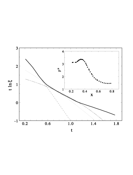
FIG. 5.: $t\ln\xi$ vs $t$ for $S=1$: fits of the PQSCHA curve (full line) with Eq. (4) in the temperature interval $[x,1.7]$ with $x=0.2$ (dashed line), $0.46$ (dotted line) and $0.56$ (dash-dotted line). The inset shows $\rho\equiv 2\pi\rho/\widetilde{S}^{2}$ as from fits in the temperature interval $[x,1.7]$ as a function of $x$.

From this analysis we conclude that the CHN-HN theory does not describe the QHAF when $\xi\leq 10^{5}$, i.e. for $t\geq 0.2$ for $S=1$ and, more in general, for $t\geq t_{0}$ where $t_{0}$ is such that $\xi_{\rm cl}(t_{0}/\theta(t_{0}))\simeq 10^{5}$ for any $S\geq 1$; the only reason why Eq. (4) seems to reproduce the experimental data is that the temperature range where the fit is carried out is small enough not to show significant deviations.

The CHN-HN theory is in fact already known to describe the QHAF only at sufficiently low temperatures, but no quantitative indication is given about the actual range of validity, save the fact that this is narrower for larger spin. What our work clearly shows is that such range of validity, for $S\geq 1$, does not overlap with the region where experimental and QMC data are available; in other terms, such data are not described by the three-loop renormalization-group expressions relative to the QNL$\sigma$M.

Although our analysis cannot be extended to all temperatures in the $S=1/2$ case, we point out that conclusions similar to ours have been recently drawn by Beard et al.[12] from their low-temperature QMC results. On the other hand, Kim and Troyer, who also performed QMC simulations on the 2DQHAF with $S=1/2$, claim[13] that their results are in ”excellent agreement” with the QNL$\sigma$M field-theory predictions. Nevertheless, such agreement involves unstable fitting procedures; in particular, the uniform susceptibility $\chi_{\rm u}$ can be fitted to the CHN-HN expression only for $t\leq 0.23$ while for the correlation length the restriction $\xi\geq 39.2$ (i.e. $t\leq 0.27$) is necessary to make the fit stable but not even sufficient to let the resulting values of $\rho$ and $c$ coincide with those obtained by fitting $\chi_{\rm u}$. In fact we think that the results presented by Kim and Troyer, which moreover extend to temperatures not as low as those studied by Beard et al., do not ”confirm the validity of the mapping from the QHAF to the NL$\sigma$M”, but rather suggest that also for $S=1/2$ the CHN-HN formulas do not properly describe the behaviour of the 2DQHAF for $t\gtrsim 0.25$, i.e., in the temperature region where most experimental and QMC data are available.

We are grateful to Prof. R.J. Birgeneau and to Y.S. Lee (MIT) for fruitful exchanges and for providing us with experimental data prior to publication.

REFERENCES

- [1] A. Sokol and D. Pines, Phys. Rev. Lett. 71, 2813 (1993).
- [2] S. Chakravarty, B. I. Halperin, and D. R. Nelson, Phys. Rev. B 39, 2344 (1989).
- [3] P. Hasenfratz and F. Niedermayer, Phys. Lett. B 268, 231 (1991).
- [4] N. Elstner et al., Phys. Rev. Lett. 75, 938 (1995); N. Elstner, Int. J. Mod. Phys. B 11, 1753 (1997).
- [5] A. Cuccoli, R. Giachetti, V. Tognetti, R. Vaia, and P. Verrucchi, J. Phys., Condens. Matter 7, 7891 (1995).
- [6] A. Cuccoli, V. Tognetti, R. Vaia, and P. Verrucchi Phys. Rev. Lett. 77, 3439 (1996), Phys. Rev. B 56, 14456 (1997).
- [7] A. Cuccoli, V. Tognetti, R. Vaia, and P. Verrucchi, Phys. Rev. Lett. 79, 1584 (1997).
- [8] K. Harada, M. Troyer, and N. Kawashima, J. Phys. Soc. Jap. 67 (in press, 1998).
- [9] S. Fulton, R. A. Cowley, A. Desert, and T. Mason, J. Phys. Condens. Matter 6, 6679 (1994).
- [10] Y. S. Lee, private communication.
- [11] R. J. Birgeneau, Phys. Rev. B 41, 2514 (1990).
- [12] B. B. Beard, R. J. Birgeneau, M. Greven, and U.-J. Wiese, Phys. Rev. Lett. 80, 1742 (1998).
- [13] J.-K. Kim and M. Troyer, Phys. Rev. Lett. 12, 2705 (1998).