A magnetic model for the incommensurate I phase of spin-Peierls systems

Abstract

A magnetic model is proposed for describing the incommensurate I phase of spin-Peierls systems. Based on the harmonicity of the lattice distortion, its main ingredient is that the distortion of the lattice adjusts to the average magnetization such that the system is always gapful. The presence of dynamical incommensurabilities in the fluctuation spectra is also predicted. Recent experimental results for CuGeO₃ obtained by NMR, ESR and light scattering absorption are well understood within this model.

Since the discovery of the inorganic compound CuGeO₃ [1], much work is devoted to the spin-Peierls transition, which is to be viewed as a magneto-elastic distortion induced by quantum magnetic fluctuations [2], [3]. It is usually observed in $s=1/2$ antiferromagnetic (AF) chains with isotropic spin-spin interactions. For such uniform chains — the corresponding lattice structure defines the U phase of the system — the interplay between spins and phonons gives rise to a lattice distortion at low temperature ($T\ll J$). Depending on the value of the applied magnetic field $H$, this distortion results in a new lattice structure which remains commensurate or becomes incommensurate. In low fields, the distortion corresponds to a lattice dimerisation — this structure defines the D phase. In large fields, the lattice incommensurability — which defines the I phase — increases with H [2]. Our purpose is to discuss for that I phase the properties of a model Hamiltonian able to describe the features observed experimentally. Comparisons with recent data obtained on CuGeO₃ are finally presented.

As a result of the incommensurate lattice distortion, the magnetic Hamiltonian in the I phase should display similar incommensurate periodicities. For $H>H_{c}$, where $H_{c}$ is the critical field of the first order transition between the D and I phases, we propose to describe the exchange coupling by the following Hamiltonian

$$H=J\sum_{i}[1-\delta_{1}\cos(qr_{i})]S_{i}S_{i+1}$$ (1)

where $\delta_{1}$ is the “alternation” of the next-nearest exchange coupling $J$ and $q$ the wavevector characterizing the magnetic modulation. Higher anharmonicities could easily be accounted for by adding terms $-\delta_{n}\cos(nqr_{i})$ — with $n$ odd integer — in the square bracket of (1). For $q=\pi$, the modulation is commensurate and the D phase is recovered. The case $\delta_{1}=0$ in (1) corresponds to the U phase. In the I phase, $q\neq\pi$ holds and we define $q=d+\pi$ where $d$ evaluates the lattice incommensurability, which is related to the average magnetization per site $\langle m\rangle=N^{-1}\sum_{i}m_{i}$ ($N$ is the system size). In the $XY$ limit of (1), for $\langle m\rangle\neq 0$, the model is equivalent to tight-binding fermions with the creation (annihilation) operators $c_{i}^{\dagger}\;(c_{i})$ [6]-[8]. When an infinitesimal spin-lattice interaction $g$ is present, instabilities occur in the system [2]. The largest one develops at $q=2k_{\rm F}=2\pi\langle m\rangle+\pi$, where the magnetic incommensurability $d=2\pi\langle m\rangle$ is created. Due to this instability, an energy gap $\Delta_{+}+\Delta_{-}$ opens in reciprocal space exactly at the two Fermi points as shown in fig. 1a). The states above and below these gaps stay separated since they evolve continuously on increasing $g$, i.e., no state can “jump” across the gap. This picture remains valid when interactions between fermions are taken into account — i.e., in the isotropic Heisenberg limit of (1). The corresponding chemical potential $\mu$ is smaller than the Zeeman energy $h=g\mu_{\rm B}H$, as the interactions create an internal field opposed to $H$. In the I phase, $\mu$ does not need to lie exactly in the middle of the energy gap (see fig. 1a)), i.e. $\Delta_{+}\neq\Delta_{-}$ in general. Three different gaps have to be considered: $\Delta_{+},\Delta_{-}$ and $\Delta_{0}$, which occur in the energy spectra of the spin fluctuations $S_{\perp}(q,E)$ and $S_{||}(q,E)$ observed in directions perpendicular and parallel to the applied field, respectively (see figs. 1b,c).

Since the system is gapful, there exists an infrared cutoff and a conventional perturbation treatment [8] offers a reliable approach. The local magnetization $m_{i}=\langle c_{i}^{\dagger}c_{i}\rangle-1/2$ is evaluated as follows. In the $XY$ limit, a chain of tight-binding fermions with hopping $t_{i}$ and local energies $\mu_{i}$ is considered. For each bond $i$, an effective two-site Hamiltonian $H_{i}$ and on-site and nearest-neighbor Green functions are defined via

$$H_{i}=\left(\begin{array}[]{cc}\mu_{i}+L_{i}(E)&t_{i}\\ t_{i}&\mu_{i+1}+R_{i+1}(E)\end{array}\right)\quad\mbox{and}\quad\left(\begin{array}[]{cc}G_{i;i}&G_{i;i+1}\\ G_{i+1;i}&G_{i+1;i+1}\end{array}\right)=(E-H_{i})^{-1}$$ (2)

The self-energy $L_{i}(E)$ ($R_{i+1}(E)$) takes the half-chain to the left (to the right) of bond $i$ into account. The conditions $L_{i}=t_{i-1}^{2}/(E-\mu_{i-1}-L_{i-1})$ and $R_{i}=t_{i}^{2}/(E-\mu_{i+1}-R_{i+1})$ define recursively continued fraction representations. The expectation values $\langle c_{i}^{\dagger}c_{j}\rangle$ are computed by the integral $\langle c_{i}^{\dagger}c_{j}\rangle=(2\pi)^{-1}\int_{\Gamma_{h}}G_{i;j}(E)dE$, where the complex contour $\Gamma_{h}$ contains the real interval $(-\infty,\mu]$. With $\mu$ within the gaps (see fig. 1a)), this integral is easily evaluated. In the isotropic Heisenberg model, a Hartree-Fock (HF) treatment is used. The fermionic chain is defined with $t_{i}=-J/2-sJ\langle c_{i}^{\dagger}c_{i+1}\rangle$ and $\mu_{i}=h-sJ(m_{i-1}+m_{i+1})$ [8]. The renormalization $s<1$ is assumed to be independent of $d$ and $H$ for small fields ($h\ll J$). It is chosen as in ref. [8], such that in the D phase — the $h,d=0$ limit of our model — $\Delta_{0}=\Delta_{+}=\Delta_{-}$. The self-consistent HF calculation is done here with full spatial dependence unlike the approach of Fujita and Machida (FM) [9] where only a constant Fock term is considered. In the $XY$ limit, one obtains the results shown in fig. 2a. The local magnetization $m_{i}$ has an alternating part and a slowly varying one, which is spatially modulated with periodicity L/2 ($L=2\pi/d$). With interactions between fermions — i.e. in the isotropic Heisenberg limit of (1) — these two important features are kept. However, the $m_{i}$ become (alternately) negative — see fig. 2b) — and their amplitude is much larger. For the same model (1), we performed also density-matrix renormalisation group (DMRG) calculations on finite chains [11]. The results confirm our renormalised HF approach very well. Note that such antiparallel local magnetizations are generic to inhomogeneous AF chains [10].

From the fermionic dispersion sketched in fig.1a), a representation of the spin fluctuation spectra in the I phase can be proposed. Based on arguments similar to those used for uniform chains [7], [12], one is led for $S_{||}(q,E)$, and $S_{\perp}(q,E)$ to figs. 1b) and c), respectively. As in [12], one has to distinguish between $S_{-+}(q,E)=\langle S^{-}(q)[E-({\bf H}-E_{0})]^{-1}S^{+}(q)\rangle$ and $S_{+-}(q,E)=\langle S^{+}(q)[E-({\bf H}-E_{0})]^{-1}S^{-}(q)\rangle$ due to the broken spin rotation symmetry. Accordingly, $S_{\perp}(q,E)$ is defined as $S_{\perp}(q,E)=[S_{-+}(q,E)+S_{+-}(q,E)]/2$. The description for the spins is obtained through $S_{i}^{+}=c_{i}^{\dagger}\exp[i\pi\sum_{l=-\infty}^{i-1}(1-c_{l}^{\dagger}c_{l})]$. In mean-field treatment, this phase factor can be written as $\approx\exp[i\pi\sum_{l=-\infty}^{i-1}(1-\langle c_{l}^{\dagger}c_{l}\rangle)]$. With $\langle c_{l}^{\dagger}c_{l}\rangle\approx 1/2+\langle m\rangle$ , it is seen to lead to a wave vector shift $(\pi-d)/2$ [7]. Hence, for a given value of $d$, the lowest energy branch of $S_{||}(q,E)$ develops an incommensurate feature at $q=\pi-d$, where the energy gap $\Delta_{0}$ occurs also (see fig. 1b). In general, $\Delta_{0}<\Delta_{+}+\Delta_{-}$. The same gap $\Delta_{0}$ appears at $q=0$, while a Zeeman shift $h$ develops at $q=\pi$ (as in the U phase [12], it implies $\mu=h/2$). For $S_{\perp}(q,E)$ (fig. 1c), similar spectra are obtained but shifted by $\pi$, with, however, the occurrence of the gaps $\Delta_{+}$ and $\Delta_{-}$ at $q=d$. The Zeeman shift is found now at the center of the Brillouin zone ($q=0$). In the inset of fig. 1b),c), the gap $\Delta_{+}+\Delta_{-}$ is calculated as a function of $\langle m\rangle$ for the values $J=120$K, $\delta_{1}=0.12$ (corresponding to CuGeO₃ [3]) and $\delta_{3}=-0.07\delta_{1}$ (see below). Renormalized HF (solid line) and DMRG (circles) results are in qualitative agreement. By DMRG, it was also verified that $\Delta_{+}$ and $\Delta_{-}$ are indeed different, but of the same order of magnitude as in fig. 1c). The same approaches correctly predict for the D phase [8] a triplet excited state giving a unique gap for $H=0$: $\Delta_{0}=\Delta_{+}=\Delta_{-}\sim 0.37J\sim 44$K [13]. For $H\neq 0$, a Zeeman splitting occurs and three branches are observed as in CuGeO₃ [3].

The lattice incommensurability in the I phase of CuGeO₃ has been established by X-ray measurements [4]. A small anharmonicity has also been observed [5]. However, the intensity ratio between the first and the third harmonic super-lattice peaks is small ($I_{3}/I_{1}\sim 1/200$ [5]), which let us expect only small anharmonicities in the exchange coupling ($\delta_{3}/\delta_{1}=-\sqrt{I_{3}/I_{1}}\sim-0.07$). Frustrating next-nearest neighbor interactions $J_{2}$ ($>0$) have also been considered by DMRG. As shown in fig. 2b) for $\alpha=J_{2}/J=0.35$ [15] and for the same gap in the D phase ($E\sim 44$K) the results do not change very much. For the local magnetization $m_{i}$ in the I phase, we refer to recent high field nuclear magnetic resonance (NMR) measurements [16]. Above $H_{c}$ ($\sim 12.5$T in CuGeO₃) and below $T_{\rm sp}$ — $T_{\rm sp}$($\sim 10$K for $H\sim 15$T) is the critical temperature of the second order transition between the U and I phases — a distribution of the $m_{i}$ develops in the crystal. Below 4K, the NMR spectra (fig. 4 in [16]) become practically $T$ independent. In other words, the distribution of the local magnetization becomes quasi-static, and our $T=0$ calculation can be used. In [16], the NMR data were analyzed within the FM soliton model [9]. In that model, the lattice distortion refers explicitly to the sine-Gordon equation (which predicts too large $\delta_{3}/\delta_{1}$ ratios [5]) and the spin system is treated in the $XY$ limit except for a constant Fock renormalization of the coupling (for the D phase, the $XY$ limit predicts only a doublet state, not a triplet as observed in CuGeO₃ [3]). The FM approach is therefore inadequate for CuGeO₃. As shown in fig. 2b), the isotropic Heisenberg limit of (1) predicts a strongly negative part for $m_{i}$, which seems to contradict the NMR data [16] where the distribution of the local field is observed to be mainly positive and to have a much smaller amplitude ($\Delta S^{z}=S^{z}_{\rm max}-S^{z}_{\rm min}\sim 0.065$). This important reduction of the experimental value of $\Delta S^{z}$ can be explained by the zero-point motion of the so-called phasons [17]. Such gapless excitations are linked to the possibility for the incommensurate distortion to slide along the chain without energy cost. This non-adiabatic effect induces “oscillations” of the magnetic pattern, which reduce the alternating component of $m_{i}$ and result in an averaging over adjacent sites as $m_{i}^{\rm eff}=(1-2\gamma)m_{i}+\gamma(m_{i+1}+m_{i-1})$. In the present work, $\gamma$ is used as a fit parameter, though a quantitative evaluation of the averaging, which is to be presented elsewhere, gives correct orders of magnitude. From the diamond data in fig. 2b) ($\alpha=0$, i.e. no frustration) one obtains for $\gamma=0.20$ the effective local magnetization depicted in fig. 2c). From the square data ($\alpha=0.35$) of fig. 2b) almost identical results (not shown) are obtained for $\gamma=0.19$. The averaging restores a mainly positive distribution, which is remarkably similar to that obtained in the $XY$ limit (compare figs. 2a) and c)). Following the same procedure as in [16], we obtain from fig. 2c) the NMR lineshapes displayed in fig. 3. A reasonable agreement is achieved for $\delta_{1}=0.12$, a result consistent with the value determined previously for CuGeO₃ [14]. For the intrinsic damping of the NMR line, we took $\sigma=0.035$T. This damping partly results from the experimental procedure since, in [16], the NMR signal was recorded as a function of $H$. During the field sweep, the incommensurability $d$ is varied, changing continuously the distribution of the $m_{i}$. This could explain the apparent “training” observed at low and high fields.

Concerning the spin dynamics in the I phase, we refer to inelastic Raman scattering (IRS) [18], [19] and electron spin resonance (ESR) [20] measurements performed in CuGeO₃ well above $H_{c}$. Concerning IRS, for any field values a striking result is obtained: a peak at $E\sim 230$ cm^-1 is observed in all the three phases [18], [19]. Such a peak occurs when the density of states of elementary excitations becomes large. In the D phase, it corresponds to (twice) the maximum of the triplet $S=1$ elementary excitations (fig.1a) in [18]), and in the U phase, to (twice) the maximum ($E_{\rm max}$) of the low energy spinon branch (fig.1b) in [18]). The peak observed in the I phase (fig. 2 in [19]) is noticeably similar to the peak in the U phase. This strongly supports the representations proposed in figs. 1b) and c) where both the U and I phases are represented: at high energy, the excitation branches behave similarly, with the same $E_{\rm max}$ and therefore the same density of states. In an ESR measurement, the $q=0$ mode of $S_{\perp}(q,E)$ is directly probed. In high fields, a remarkable behavior of the ESR signal has been reported [20]: no change on its position and lineshape occurs when the U-I transition line is crossed (fig. 1 in [20]). This result supports well our conjecture presented in fig.1c) since the $q=0$ mode undergoes the same Zeeman shift $h$ in the two phases. At $T_{\rm sp}$, the only dynamical changes occur in the low energy part of the spectra, with the opening of the energy gaps $\Delta_{+}$ and $\Delta_{-}$.

In conclusion, a magnetic Hamiltonian is proposed to describe the properties of the I phase of a spin-Peierls system [21]. The lattice distortion is considered to result mainly in a modulation of the exchange alternation. Both the local magnetization distribution and the dynamical properties known at present for the I phase of CuGeO₃ are well explained by this model. It predicts the adiabatic I phase to be characterized at low energy by two important features: the presence of a dynamical incommensurability (as in the U phase) and the opening of energy gaps (as in the D phase). Varying the external field tends to reduce either $\Delta_{+}$ or $\Delta_{-}$. The whole spin-lattice system, however, responds by changing its global modulation in order to minimize its total energy so that eventually none of the gaps closes.

***

We would like to thank Y. Fagot-Revurat, H. J. Schulz and Th. Nattermann for helpful discussions. One of us (GSU) acknowledges the hospitality of Laboratoire de Physique des Solides, Université Paris-Sud, Orsay, where this work was initiated, and the financial support of the Deutsche Forschungsgemeinschaft (individual grant and SFB 341).

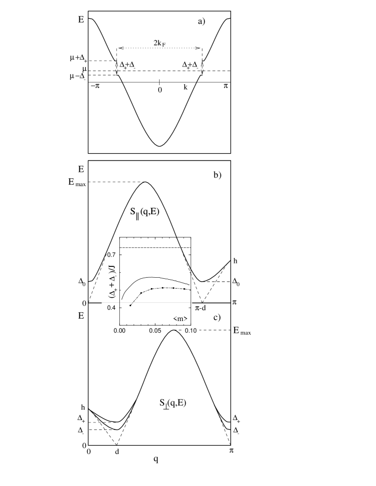
Fig. 1.–: a) Fermionic dispersion for Hamiltonian (1). The Fermi energy is denoted by $\mu$; b) and c) dispersions of the spin excitations in $S_{||}(q,E)$ and $S_{\perp}(q,E)$ for the I and U phases (solid and dashed lines, respectively). For $h\ll J,E_{\rm Max}/J\sim(\pi/2)$. Inset: dependence of the energy gap $\Delta_{+}+\Delta_{-}$ as a function of the incommensurability $d$ (solid line), for $\delta_{1}=0.12$ [14], $\delta_{3}=-0.07\delta_{1}$ and $\alpha=0$ (see text). The dots depict DMRG results for a 66 site chain. The dashed line is twice the gap value ($0.37J$) determined for the D phase [14].

Fig. 2.–: a) Local magnetization versus site number in the $XY$ limit of Hamiltonian (1) for $L(=2\pi/d)\sim 66$ (as in [16]), $\delta_{1}=0.12,\delta_{3}=-0.07\delta_{1}$ and $\alpha=0$; b) diamonds: as previously but in the Heisenberg limit of (1) (DMRG provides almost identical results); squares: DMRG results (same gap but $\alpha=0.35,\delta_{1}=0.033,\delta_{3}=-0.07\delta_{1}$ for a 66 site chains ; c) the effective local magnetization in the isotropic Heisenberg limit for $\gamma=0.20$ (see text). In a), the dashed and dot-dashed lines correspond to the FM model [9] calculated for the value $k=0.9$ ($k$ is the modulus of the elliptic Jacobi function; the offset occuring in the FM description is determined by $\langle m\rangle=1/L$ and $L=66$. Full symbols: odd sites; empty symbols: even sites; curves through symbols are guides to the eye.

Fig. 3.–: NMR lineshapes evaluated from the distribution of the local magnetization displayed on fig. 2c), for different values of $\delta_{1}$ and $\delta_{3}=-0.07\delta_{1}$. The internal NMR damping is $\sigma=0.035$T (see text).

References

- [1] M. Hase et al., Phys. Rev. Lett., 70 (1993) 3651.
- [2] For a general review on the spin-Peierls transition see: J.W. Bray et al., in Extended Linear Chain Compounds,, edited by J.S. Miller, Vol. 3 (Plenum Press, New York) 1983.
- [3] For a review on CuGeO3 see: J.P. Boucher and L.P. Regnault, J. Phys. I, 6 (1996) 1939.
- [4] V. Kiryukhin and B. Keimer, Phys. Rev. B, 52 (1996) 704.
- [5] V. Kiryukhin et al., Phys. Rev. Lett., 76 (1996) 4608.
- [6] P. Jordan and E. Wigner, Z. Phys., 47 (1928) 42.
- [7] L.N. Bulaevskii, Soviet Phys. JETP, 16 (1963) 685; E. Pytte, Phys. Rev. B, 10 (1974) 4637.
- [8] G.S. Uhrig and H.J. Schulz, Phys. Rev. B, 54 (1996) 9624.
- [9] M. Fujita and K. Machida, J. Phys. C, 21 (1988) 5813.
- [10] S. Eggert and I. Affleck, Phys. Rev. Lett., 75 (1995) 934; Gelfand and E.F. Gloeggler, Phys. Rev. B, 55 (1997) 11372.
- [11] F. Schönfeld et al., submitted to Europhys. J. B and cond-mat/9803084.
- [12] G. Müller et al., Phys. Rev. B, 24 (1981) 1429.
- [13] This value agrees well with the experiments in CuGeO3 [3]: calculated for a purely 1D system, it should be compared not to the lowest gap ( K) but to an “average gap”, the averaging being made over the dispersions transverse to the chains [14].
- [14] G.S. Uhrig, Phys. Rev. Lett., 79 (1997) 163.
- [15] J. Riera and A. Dobry, Phys. Rev. B, 51 (1995) 16098; G. Castilla et al., Phys. Rev. Lett., 75 (1996)1823; K. Fabricius et al., Phys. Rev. B, 57 (1998) 1102.
- [16] Y. Fagot-Revurat et al., Phys. Rev. Lett., 77 (1996) 1861.
- [17] S.M. Bhattacharjee, T. Nattermann and C. Ronnewinkel, cond-mat/9711091.
- [18] P.H.M. van Loosdrecht et al., Phys. Rev. Lett., 76 (1996) 311.
- [19] P.H.M. van Loosdrecht et al., J. Appl. Phys., 79 (1996) 5395.
- [20] W. Palme et al., Phys. Rev. Lett., 76 (1996) 4817.
- [21] In the I phase, we do not expect important changes for the local magnetization from the interchain couplings. They will, however, reduce the gap values as they do in the D phase [14].