The Randomly Driven Ising Ferromagnet
Part II: One and two dimensions
Abstract
We consider the behavior of an Ising ferromagnet obeying the Glauber dynamics under the influence of a fast switching, random external field. In Part I, we introduced a general formalism for describing such systems and presented the mean-field theory. In this article we derive results for the one dimensional case, which can be only partially solved. Monte Carlo simulations performed on a square lattice indicate that the main features of the mean field theory survive the presence of strong fluctuations.
pacs:
PACS numbers: 05.50+g 05.70.Jk 64.60Cn 68.35.Rh 75.10.H 82.20.MThis paper considers the randomly driven Ising model (RDIM), introduced and discussed from a general point of view in Part I[1], in one and two dimensions. The main interest in studying such highly nonlinear nonequilibrium statistical physical systems lies in their possible applications for storage and other information processing tasks. Many biological systems, especially networks of real neurons, share common features with the RDIM in that they form strongly coupled systems driven by external stimuli acting in unison over a macroscopic number of elements in characteristic times shorter than the typical system relaxation time. Therefore, the Gaussian or Poissonian external “noise” is transformed radically within the coupled system, leading to a “correlated noise” with a lot of “strange” properties. The mean field theory was developed in Part I [1] for a random binary switching external field. Applications to cortical neurons will be discussed elsewhere.
The order parameter of the RDIM is a nonequilibrium stationary magnetization distribution, which undergoes a symmetry breaking bifurcation at some critical field strength. The analytic structure of this distribution also changes in character as a function of the temperature and field parameters. Hence, transitions between a singular function with fractal support to a singular function with euclidean support and further, to an absolutely continuous distribution can be observed. They can be seen in finite size effects and in the variance (the fluctuations) of the free energy. Similar transitions can be seen also in one dimension. However, the critical lower dimensionality of the RDIM remains one. Although the static critical exponent is a function of the field/temperature ratio, the dynamic exponent remains unchanged. Some simple arguments will be given, supporting these results.
The situation is much more difficult in two-dimensions, where only a Monte Carlo simulation approach was possible. The main difficulty is that computing the stationary properties of the system requires a large population of different trajectories. We found that it is more convenient to use systems of moderate size than to rely on only few dynamic trajectories. Even so, the simulations require a vast amount of computer resources. We solved this problem by using the Siemens-Nixdorf neurocomputer SYNAPSE-1N110 for quite a different task than what it was conceived for. This machine is basically a matrix-computer, allowing us to run many different systems in parallel. Even so, we were able only to determine roughly the phase diagram itself: we have no means at the moment for calculating the critical exponents.
The paper is organized as following: in Section I we consider the one dimensional case. Although it cannot be fully solved, many interesting exact results can be derived. Section II deals with the Monte Carlo simulations we performed on finite square lattices. Many features of the mean-field dynamics are shown to survive the strong fluctuations characteristic to two dimensional systems. However, in contrast to the mean-field approach, the two dimensional model displays also an interesting spatial structure related to droplet dynamics. Comparisons between mean-field theory and two-dimensional results are systematically presented, including some preliminary results for hysteresis. Finally, we discuss our results in Section III.
I RDIM in one dimension
A The Master Equation
In his pioneering work, Glauber [2] defined a stochastic dynamics where only single spin flips are allowed and hence neither the magnetization (the order parameter) nor the energy is preserved (model A universality class, see [3]). Although introduced mainly for mathematical convenience, this dynamics is believed to describe appropriately many Ising-like systems.
The energy of an Ising chain with periodic boundary conditions is given by
| (1) |
Following the notation of Part I[1] we denote by the vector a given configuration of spins and by the same configuration but with the spin flipped. The external field is sampled from at time intervals of length ,
| (2) |
As explained in Part I, the Master Equation has the form
| (3) | |||||
| (4) |
where is the transition rate from a configuration into the state where only the -th spin is flipped, .
Strictly speaking, the system we are going to consider here will never reach the equilibrium Boltzmann distribution , where . Nevertheless, we require the detailed balance condition to be fulfilled for a constant value of the external field.
The transition probability is determined by the constraint of detailed balance only up to a positive arbitrary function of the neighboring spins, . Since in one dimension the phase transition is at , the choice of the transition probability influences the analytic form of the critical singularities [4]. In what follows we will use the form
| (5) |
where , , sets the time constant, and denotes next neighbor pairs. Glauber introduced this form for but used a slightly different one for . In one dimension one has then
| (6) |
For the Liouville operator can be mapped onto a free-fermion spin-chain Hamiltonian [5]. This explains why the equations for the averaged spin products, , decouple in subspaces which can be diagonalized by appropriate Fourier transformations. As shown below, this property is inherited by the first moments, of the stationary distribution .
B Magnetization and correlation functions
Consider, for example, the time evolution of the local magnetization
| (7) |
which can be obtained from (4) as
| (8) |
In order to make the relationship to chaotic maps more evident, we use now the ‘coarse grained’ form[1] of (4). Formally, this procedure corresponds to a forward Euler discretization of (8), setting the time step equal to , and measuring time in units of :
| (9) | |||||
| (10) |
where , , and
| (11) | |||||
| (12) | |||||
| (13) |
Similarly, for the correlation function
| (14) |
one obtains
| (15) |
leading to the map
| (16) |
where the time unit is now set to . These recursions can be written again in terms of the variables , and , Eqs. (11-13).
For one has and, as shown by Glauber [2], the slowest relaxation time equals the inverse of the smallest eigenvalue of the magnetization subspace, Eq. (8). This relaxation time diverges with the square of the static correlation length (the dynamic critical exponent is ).
For the binary field distribution of (2) the map of the local magnetization (10) has two branches:
| (17) |
where it is implicitly assumed that the time needed to switch the field is negligible, .
From Eq. (17) it is evident that the map for the local magnetization couples to a two-spin correlation, which in turn couples to higher order correlations, etc. Hence, the full dynamic map lives in a dimensional space, as stated in Part I[1].
Nevertheless, some partial results can be obtained for the stationary distribution. Define a ‘thermal’ and a ‘dynamical’ average, resp. . In the stationary state one has for any spin-function . The average of the local magnetization obeys
| (18) |
where (recall that , )
| (19) |
For the translation invariant magnetization and the two-spin correlation function one obtains equations formally similar to the ones solved by Glauber [2]. From (18), except for , the magnetization vanishes. The stationary two-spin correlation function obeys
| (20) |
which leads to
| (21) |
In general, when expressing the Frobenius-Perron operator in the basis formed by all moments of spin-products , the subspace of the first moments () is closed and can be diagonalized by a Fourier transform. The remaining part, however, is intractable. For example, the second moment of the magnetization reads
| (22) |
and couples both to the first and to the second moment of the translation invariant correlation functions, and , respectively.
C The phase transition
As expected, in the stationary state the odd moments of the magnetization vanish at . By expanding and at low temperature one obtains after straightforward calculations that close to the correlation length is in leading order
| (23) |
where and is defined as in Eq. (2). Hence, in one dimension the RDIM has a critical line with continuously changing singularities at for . The slowest relaxation time corresponds to the magnetization (order parameter) decay and can be computed as
| (24) |
Consider first the case of a strong field, . The field will align all spins in one iteration step, as evident from Eq. (24). Hence, the spins are almost always parallel to the driving field. Since vanishes, there is no spontaneously broken symmetry and due to the symmetry of the field distribution, .
For fields smaller than the critical field one obtains a true symmetry breaking ferromagnetic phase. Interesting enough, while the divergence of the correlation length decreases continuously according to Eq. (23), the critical dynamic exponent remains up to and including . A physical argument explaining this result is presented below.
D Kink dynamics at
Consider now the transition probability at , Eq. (6), which is a function of the three spins , , and . Let us call an interface between two oppositely oriented spin domains a kink. If and each kink performs a random walk, moving with equal probability to the left or to the right. When two kinks become nearest neighbors, they annihilate because in the next time step the single spin left between them will flip with probability one.
Due to this annihilation process the number of kinks decreases steadily and in the end only very few are left. Two kinks situated at the typical distance (the correlation length) will meet via diffusive motion in the characteristic time , which explains why the critical dynamic index is . The situation is similar if one is close to (but not at) .
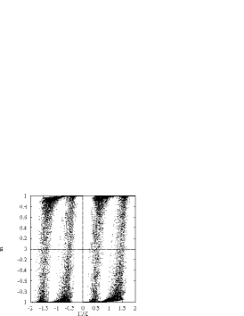
How does this picture change if we switch on the random external field ()? The domains parallel to the external field start growing - both ends of such a cluster will move outwards. Once the field changes sign, these domains shrink again and the clusters of oppositely aligned spins grow. During a longer period of time these effects compensate each other and the surviving kinks perform effectively a random walk. However, the annihilation rate of kink-pairs is highly increased. Assume, for example, that after iteration steps the external field had the value -times. The probability for this to happen is given by the Bernoulli distribution, . During this time, a down-oriented domain whose original length was shrinks on average by , where both kinks associated with the ends of the domain have moved inward during each of the time steps with probability and outward with probability . Hence, if , the domain will be eliminated. is a function of , e.g. . Due to the depletion of small clusters, the number of kinks decreases much faster than in the absence of the external field. This effect is illustrated by a numerical simulation in Fig. 1, showing the dynamics of walls for and , respectively.
Once only a few large clusters remain, however, their width becomes macroscopic. On this scale the kinks perform again a random walk and asymptotically one regains .
At finite temperatures, however, the presence of the field term facilitates the nucleation of new clusters, so that the correlation length (23) (the mean cluster size) is less divergent when .
E The magnetization distribution
Consider again the map (17). In the translational invariant sector one has
| (25) |
As already discussed, the magnetization couples to the correlation function , etc. A simple approximation to decouple the magnetization sector is using for the stationary value . The resulting map corresponds to a Bernoulli-shift [6] and is shown graphically in Fig. 2. If the gap between the two branches is positive
| (26) |
the corresponding stationary magnetization distribution is a Cantor set.
Since , , are positive and for ferromagnetic interactions, the demarcation line between a fractal and a nonfractal magnetization distribution is given by
| (27) |
independently of the actual value might have. The time dependence of induces nonlinearities in the map. Therefore, although the distribution remains fractal for , in general it is not a homogeneous Cantor set.
II Monte Carlo simulations in two dimensions
We simulated the RDIM on a two dimensional square lattice on the neurocomputer SYNAPSE-1/N110. In the following sections we first describe a Monte Carlo Algorithm (MCA) designed to make use of the computational power of SYNAPSE-1 and then present our numerical results. They include a phase diagram in the H-K-plane, magnetization distributions in the para- and ferromagnetic regime, and a series of snapshots documenting the behavior of the system.
A The algorithm
SYNAPSE-1 is a workstation-driven coprocessor consisting of a systolic array of eight MA16 Neural Signal Processors. It was kindly put at our disposal by the ZFE of Siemens AG. Its hardware was designed to tackle typical problems encountered when simulating neural networks, namely calculations involving very large matrices. In order to efficiently make use of the C++-library interface supplied with SYNAPSE-1 for the RDIM, we devised a MCA that simulates multiples of eight lattices in parallel.
Consider a square lattice of spins of linear dimension , where numbers the system and denotes the lattice position. Each of eight lattices is represented as a column vector by renumbering indices . The eight systems can thus be treated as one -matrix. By setting for and for we enforce helical boundary conditions. The neighbors of spin are .
In order to avoid metastable states induced by a simultaneous update of neighboring spins we split the lattices into black and white sites in a checkerboard fashion, leading to two matrices encoding the eight systems. Note that when a lattice is divided up in this fashion, if is odd, the sites in the first and last row have neighbors of their own color. If is even, the same is true for the first and last column of the lattice. For technical reasons we chose to be odd.
To further simplify the updating scheme, a copy of the first and last components of each lattice are included at the end respectively beginning of each column vector. A Monte Carlo step now consists of a parallel update of all black sites followed by an update of all white sites (or vice versa).
From the well known Glauber dynamic rule Eq. (5), a spin is flipped under the following condition. Given a random number drawn from a uniform distribution, spin is updated according to
| (28) |
Usually, spins are either treated sequentially or chosen randomly. SYNAPSE-1 permits the parallel generation of (pseudo-) random numbers in a single Elementary Operation (ELOP) which can be piped through a function lookup table at no extra computational cost. For this reason we transform the flip condition Eq. (28) into
| (29) |
where is drawn from a uniform distribution in . The RHS of the flip condition is evaluated in two ELOPs: One to generate a matrix of random numbers piped through the function and one weighted matrix subtraction. The LHS also takes two ELOPs to calculate from the “black” and “white” matrices. Two further ELOPs are required to construct and evaluate a flip indicator matrix. Some more operations are necessary to fix boundary conditions and to evaluate the mean lattice magnetizations. This procedure is applied sequentially first to the matrix holding the “black” spins and then to the “white” one to accomplish a complete Monte Carlo step.
Initially, the spins in a lattice are set to with probability and with probability , where different values of can be used for each lattice in one simulation run. The results for systems of linear dimension are initialized with 0, 0.2, 0.4, 0.5, 0.6, 0.8, and 1, in addition, there is one lattice in which the top half of all spins is set to and the bottom half to . The external driving field is the same for each system. Simulations at smaller consist of 64 systems initialized with , but each with its own driving field trajectory.
Temperature is measured in units of the critical temperature, , where of the standard two dimensional Ising model, i.e. corresponds to the critical temperature for .
B Dynamics and phase diagram
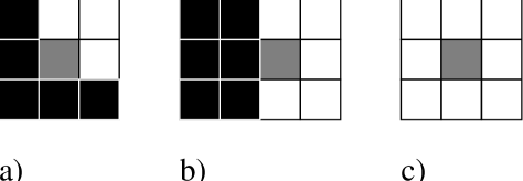
In order to understand the dynamics of the two-dimensional RDIM in more detail, it is useful to consider first what happens to a cluster of parallel spins at , in analogy to kink dynamics for the one dimensional case. Transition rates at are either , or . Recalling that is measured in units of , define . Consider now a square cluster of parallel spins under the influence of an anti-parallel external field. First, if , the spins at the corners of the cluster flip with probability , all other remain anti-parallel to the field (as shown in Fig. 3 a). Thus the cluster disappears if the external field remains constant for consecutive steps. Secondly, if , such a cluster will be destroyed in steps, due to the fact that all but inner spins will flip with . Thirdly, at we arrive at a driven paramagnetic phase. Regardless of their position, all spins will flip into the direction of the driving field with . For the case of ,,or , corner, edge, and inner spins flip with . This implies that, e.g. for a strong driving field with , nucleation flips (see Fig. 3 c) may take place inside the cluster, creating magnetic swiss cheese.
The transition probabilities of the processes shown in Fig. 3 increase with increasing field strength. At small fields the a)-type flip is prevalent, resulting in a radial growth (shrinkage) of clusters. Although energetically more expensive, the b)-type flip has a large entropy contribution and results in long-wavelength growth of flat domain walls. The nucleation process shown in flip c) has the smallest probability.
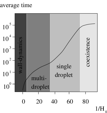
What happens when switching instantly the field from the equilibrium state at into the unfavorable direction ? The system relaxes from the now metastable state to the new equilibrium value. Obviously, the lifetime of the metastable state depends on the strength of the applied field. This scenario has been discussed in detail in the ferromagnetic phase using droplet theory and Monte Carlo simulations (see, for example, [7]). Here, four distinct field intervals, shown schematically in Fig. 4 were, identified in which the lifetimes markedly differ due to different decay mechanisms. A numerical result for is shown in Fig. 5, where we approximated the metastable lifetimes by measuring the average first passage times (FPT) from to in Monte Carlo steps. Figs. 6 and 7 show examples of the time development of the magnetization from the metastable state to th new equilibrium for the mean field and 2D model.
We calculated numerically a phase diagram in the plane for the 2D RDIM, Fig 8. Similar to the mean field and one dimensional model, there is a paramagnetic, a ferromagnetic (and a driven paramagnetic) phase. Note that for , the phase boundary should remain below . We are currently in no position to assess this. Also, the behavior around doesn’t seem to correspond to the first order dynamic freezing transition seen in the mean field theory, rather a second order transition is likely.
C The paramagnetic phase
If the external field is above its critical value, , the stationary phase of the RDIM is paramagnetic. In this phase the system relaxes relatively fast to the equilibrium state, except close to , where critical slowing down sets in due to the type-I intermittency effects discussed in the previous section.
This behavior of the average magnetization is shown in Fig. 7 and is probably enhanced by local correlations not taken into account in the mean field approximation. If the random field is switched on, close but above the critical slowing down is dramatically enhanced. Further away from the phase transition point the dynamics is - similarly to the one-dimensional case - determined by the nucleation and radial growth (shrinking) of droplet-like clusters.
As expected from the mean-field results, the RDIM can display a fractal magnetization distribution at higher fields. This is shown in Fig. 9. Thermal fluctuations and finite size effects wash out the fine structure of the multifractal magnetization distribution predicted by the mean-field calculations. However, the presence of sharp peaks in the distribution (and their scaling behavior) demonstrates that some of the main features of the magnetization distribution survive the thermal fluctuations.
These peaks are related to long-lived droplets whose radius is large enough to allow them to stay alive even when a long series of unfavorable external field draws makes them shrink. It is, however, the competition between the two thermodynamically stable states which leads to a chaotic dynamics and strange attractors.
D The ferromagnetic phase
The situation is even more complex below . The schematic dependence of the average time spent in a thermodynamically unstable state vs. the inverse of the field strength is shown after [7] in Fig. 4.
The external-field sampling time should be chosen in either the strong or multi-droplet regime (certainly not in the coexistence regime). By varying is seems possible to explore these different dynamic mechanisms in more detail. Fig. 10 shows a simulation in the ferromagnetic phase where one can observe both a multi-droplet (series 1 and 3) and a domain-wall type (series 2) dynamics. Again, the spontaneous magnetization distribution shows well separated peaks, which can be seen in Fig. 11.
For the sake of completeness, we show also a Monte Carlo simulation of the hysteresis measurement described in Fig. 8 of Part I[1]. Only the evolution of one system initialized with spins up/down with equal probability is displayed. Again, one can see that the thermal fluctuations are smoothing only the fine scale structure of the mean-field predictions – but the main features remain intact.
The results presented here leave open many questions regarding the 2D RDIM – an in-depth study by Monte Carlo simulation lies currently beyond our means. The theory and evolution of droplets and domains in the RDIM as well as hysteretic effects remain interesting research topics.
III Summary and Discussion
In Part I and in this article we have discussed in detail the properties of a simple Ising model subject to a fast switching external field. In many ways, the situation is just the opposite as in quenched random systems. While there the defects and hence the (local) fields are frozen relative to the spin degrees of freedom, which are (in principle) free to relax, in the RDIM the external field is the fast variable compared to the interacting spin system. From a “technological” theoretical point of view the situation is, however, much easier. We expect that similar analytic results can be obtained for other random distributions as well. Strongly driven systems show rather peculiar properties, which one could use for increasing the storage properties of ferromagnetic materials. For example, it seems possible to use arithmetic coding in ‘preparing’ a semi-macroscopic ferromagnetic region to fall into a given distribution peak, as the ones shown in Fig. 9. An appropriately sensitive reading head could then discriminate between the different magnetization values. Such ‘devices’ could be tested first with the help of Monte Carlo simulations. However, the main application domain for randomly driven systems might well be in biology. Further work in that direction is under progress.
Acknowledgments
We are grateful to the ZFE, Siemens AG and U. Ramacher for the SYNAPSE-1 neurocomputer, on which the Monte Carlo simulations were performed. This work was partly supported by the DFG through SFB 517.
REFERENCES
- [1] P. Ruján and J. Hausmann, The randomly driven Ising ferromagnet, Part I: General formalism and mean field theory
- [2] R. J. Glauber, Time-dependent statistics of the Ising model, J. Math. Phys. 4 (1963) 294
- [3] For a review see: B. I. Halperin and P. C. Hohenberg, Theory of dynamic critical phenomena, Rev. Mod. Phys. 45 (1977) 435
- [4] R. Pandit, G. Forgács, and P. Ruján, Finite-size calculations for the kinetic Ising model, Phys. Rev. B 24 (1981) 1576
-
[5]
B. U. Felderhof,
Rep. Math. Phys. 1 (1970) 1
E. D. Siggia, Pseudospin formulation of kinetic Ising models, Phys. Rev. B 16 (1977) 2319 - [6] S. Grossmann and H. Horner, Long time tail correlations in discrete chaotic dynamics, Z. Phys. B 60 (1985) 79
- [7] P. A. Rikvold, H. Tomita, S. Miyashita, and S. W. Sides, Metastable lifetimes in a kinetic Ising model: dependence on field and system size, Phys. Rev. E 49 (1994) 5080


![[Uncaptioned image]](/html/cond-mat/9804233/assets/x13.png)
![[Uncaptioned image]](/html/cond-mat/9804233/assets/x14.png)