[

Elastic Properties of C and $\mbox{B}_{x}\mbox{C}_{y}\mbox{N}_{z}$ composite nanotubes

Abstract

We present a comparative study of the energetic, structural and elastic properties of carbon and composite single-wall nanotubes, including BN, $\mbox{BC}_{3}$ and $\mbox{BC}_{2}\mbox{N}$ nanotubes, using a non-orthogonal tight-binding formalism. Our calculations predict that carbon nanotubes have a higher Young modulus than any of the studied composite nanotubes, and of the same order as that found for defect-free graphene sheets. We obtain good agreement with the available experimental results.

]

Carbon nanotubes [1] were first discovered by Iijima [2] in the early nineties, as a by-product of fullerene synthesis. Since then there has been an ever-increasing interest in these new forms of carbon, partly due to their novel structures and properties, but perhaps more so due to the wealth of potentially important applications in which nanotubes could be used. Indeed many applications have already been reported, from their use as atomic-force microscope tips [3], to field emitters [4], nanoscale electronic devices [5] or hydrogen storage [6], to cite a few. But probably the highest potential of nanotubes is in connection with their exceptional mechanical properties.

After the discovery of graphitic nanotubes it was postulated that other compounds forming laminar graphite-like structures could also form nanotubes [7]. In particular, BN [8], $\mbox{BC}_{3}$ [9], $\mbox{BC}_{2}\mbox{N}$ [10] and CN [11] nanotubes were predicted on the basis of theoretical calculations. BN [12], $\mbox{BC}_{3}$ and $\mbox{BC}_{2}\mbox{N}$ [13] have since been synthesized, though some uncertainty remains as to the actual structure of $\mbox{BC}_{2}\mbox{N}$ nanotubes [14].

The mechanical properties of carbon nanotubes have been the subject of a number of theoretical [15, 16, 17, 18, 19, 20, 21] as well as experimental [22, 23, 24] studies. On the theoretical side, studies have been mostly carried out using empirical potentials, although Molina et al. [17] employed an orthogonal tight-binding model in their work. The most extensive theoretical study of the elastic properties of carbon nanotubes to date is that of Lu [21], who used an empirical pair potential model to estimate the Young modulus, Poisson ratio and other elastic constants of both single-wall and multi-wall nanotubes, as well as nanotube ropes. However, it was not possible to extend this study to composite nanotubes, given that no empirical potential models akin to that used for carbon exist for the composite systems. The behavior of carbon nanotubes subject to large axial strains has been studied by Yakobson et al. [18]. The bending of carbon nanotubes has been studied experimentally and using simulation techniques by Iijima et al. [20]. The Young modulus of carbon multi-wall nanotubes has been experimentally determined by Treacy et al. [22] using thermal vibration analysis of cantilevered tubes. They obtained a mean value of the Young modulus of $1.8\pm 1.4$ TPa. More recently, Wong et al. [23] have obtained a value of $1.28\pm 0.59$ TPa, by recording the force needed to bend anchored nanotubes using an AFM. Chopra and Zettl [24] have also used thermal vibration analysis to estimate the Young modulus of multi-wall BN nanotubes, obtaining a value of $1.22\pm 0.24$ TPa. These experimental and theoretical studies confirm the expectation that nanotubes have exceptional stiffness, and could therefore be used in the synthesis of highly resistant composite materials.

In this work we study the structural, energetic and mechanical properties of both carbon and composite nanotubes, paying special attention to the mechanical properties, since these are expected to play such an important role in many practical applications. This is the first time that such a detailed comparative study is undertaken. In the majority of the calculations reported here the atomic interactions have been modeled using a non-orthogonal tight-binding scheme due to Porezag and coworkers [25]. Tight-binding (TB) methods [26] offer a good compromise between the more accurate but much more costly first principles [27] techniques, and empirical potentials [28], which are cheaper to use, but often not transferable to configurations different to those for which they have been fitted.

In the TB scheme used here, the hopping integrals used to construct the Hamiltonian and overlap matrices are tabulated as a function of the internuclear distance on the basis of first-principles density-functional theory (DFT) calculations employing localized basis sets, retaining only one- and two-center contributions to the Hamiltonian matrix elements [25]. A minimal basis set corresponding to a single atomic-like orbital per atomic valence state is used. More details on the construction of the TB parametrisation used in this work can be found in ref. [25].

Using the non-orthogonal TB scheme briefly outlined above we have performed a series of calculations aimed at characterizing the elastic properties of single-wall nanotubes. In particular, we have considered C, BN, $\mbox{BC}_{3}$ and $\mbox{BC}_{2}\mbox{N}$ (n,n) and (n,0) (i.e. non-chiral) nanotubes. Two structures having the same stoichiometry are possible for the $\mbox{BC}_{2}\mbox{N}$ nanotubes. Only the structure known as II [10, 29] is considered here, as this is predicted to be the most stable of the two. In addition, we have performed calculations for the chiral (10,5) and (10,7) C nanotubes. We have also carried out Plane Wave (PW) pseudopotential DFT calculations within the local density approximation (LDA) for the (6,6) C and BN nanotubes, for comparison with the TB results. Our PW calculations used Troullier-Martins pseudopotentials [30]. A cut off of 40 Ry was used in the basis set, and 10 Monkhorst-Pack [27] points to sample the one-dimensional Brillouin zone. The hexagonal supercell was chosen large enough so as to ensure that the minimum distance between a tube and any of its periodic images was larger than 5.5 Å. Our TB calculations were performed using $\Gamma$-point sampling only, but using periodically repeated cells which where large enough along the axial direction so as to ensure that total energy differences were converged to an accuracy approximately equal to that achieved with the PW calculations.

The Poisson ratio is defined via the equation

$$\frac{R-R_{eq}}{R_{eq}}=-\sigma\epsilon.$$ (1)

Here, $\epsilon$ is the axial strain, $R_{eq}$ is the equilibrium tube radius, $R$ is the tube radius at strain $\epsilon$ and $\sigma$ is Poisson’s ratio. The values of $\sigma$ obtained for a number of representative tubes considered in this work are reported in Table I. Regarding the Young modulus, its conventional definition is

$$Y=\left.\frac{1}{V_{0}}\;\frac{\partial^{2}\!E}{\partial\,\epsilon^{2}}\right|_{\epsilon=0},$$ (2)

where $V_{0}$ is the equilibrium volume, and $E$ is the strain energy. In the case of a single-wall nanotube, this definition requires adopting a convention in order to define $V_{0}$, which for a hollow cylinder is given by $V_{0}=2\pi LR\delta R$, where $L$ is the length, $R$ the radius and $\delta R$ is the shell thickness. Different conventions have been adopted in the past; for example, Lu [21] recently took $\delta R=0.34$ nm, i.e. the interlayer separation in graphite, while Yakobson et al [18] took the value $\delta R=0.066$ nm. We follow a different path. Rather than adopting an ad hoc convention, we use a different magnitude to characterize the stiffness of a single-wall nanotube, which is independent of any shell thickness. We define

$$Y_{s}=\left.\frac{1}{S_{0}}\;\frac{\partial^{2}\!E}{\partial\,\epsilon^{2}}\right|_{\epsilon=0}.$$ (3)

Here, $S_{0}$ is the surface defined by the tube at equilibrium. The value of the Young modulus for a given convention value $\delta R$ is given by $Y=Y_{s}/\delta R$. In Table I we give the values obtained for $Y_{s}$ for a number of tubes.

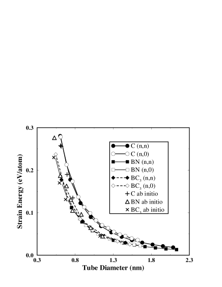
FIG. 1.: Curvature strain energy as a function of the equilibrium tube diameter, as obtained from the tight-binding calculations, for C, BN and $\mbox{BC}_{3}$ nanotubes. ab initio results are from refs. [8-10].

Our first observation is that PW and TB results give very similar answers for all the calculated properties. The differences in values of the Young modulus (calculated adopting the convention $\delta R=0.34$ nm) for the (6,6) C nanotube are of the order of 0.12 TPa.

$\mbox{B}_{x}\mbox{C}_{y}\mbox{N}_{z}$	(n,m)	$D_{eq}$ (nm)	$\sigma$	$Y_{s}$ ($\mbox{TPa}\cdot\mbox{nm}$)	$Y$ (TPa)
C	(10,0)	0.791	0.275	0.416	1.22
	(6,6)	0.820	0.247	0.415	1.22
		(0.817)		(0.371)	(1.09)
	(10,5)	1.034	0.265	0.426	1.25
	(10,7)	1.165	0.266	0.422	1.24
	(10,10)	1.360	0.256	0.423	1.24
	(20,0)	1.571	0.270	0.430	1.26
	(15,15)	2.034	0.256	0.425	1.25
BN	(10,0)	0.811	0.232	0.284	0.837
	(6,6)	0.838	0.268	0.296	0.870
		(0.823)		(0.267)	(0.784)
	(15,0)	1.206	0.246	0.298	0.876
	(10,10)	1.390	0.263	0.306	0.901
	(20,0)	1.604	0.254	0.301	0.884
	(15,15)	2.081	0.263	0.310	0.912
$\mbox{BC}_{3}$	(5,0)	0.818	0.301	0.308	0.906
	(3,3)	0.850	0.289	0.311	0.914
	(10,0)	1.630	0.282	0.313	0.922
	(6,6)	1.694	0.279	0.315	0.925
$\mbox{BC}_{2}\mbox{N}$ II	(7,0)	1.111	0.289	0.336	0.988
	(5,5)	1.370	0.287	0.343	1.008

TABLE I.: Structural and elastic properties of selected nanotubes obtained from the tight-binding calculations reported here. Young modulus values given in parenthesis were obtained from first-principles calculations. Also the value of $Y$ with the convention $\delta R=0.34$ nm is given for comparison.

It is worth pointing out that this difference is small compared to the uncertainty with which $Y$ can at present be experimentally determined for multi-wall nanotubes [22, 23, 24]. Structural properties deduced from the PW and TB calculations are also in very good agreement for both C and BN systems. The equilibrium diameter, as seen in Table I, differs by about 1 % or less. The nearest neighbor distance in the case of the (6,6) C nanotube is 1.42 Å in both the PW and TB calculations. For the BN (6,6) nanotube, the results are 1.43 Å and 1.45 Å for the PW and TB calculations, respectively.

An interesting magnitude associated with nanotubes is the curvature energy or strain energy $E_{s}$, which we define as the difference of the energy per atom in the tube and that in the corresponding infinite flat sheet. In Fig. 1 we plot the strain energy obtained from our TB calculations for C, BN and $\mbox{BC}_{3}$ nanotubes as a function of the tube diameter. It can be seen that the characteristic behavior $E_{s}\propto 1/D^{2}$, where $D$ is the tube diameter, is obtained. Our calculations indicate that the strain energy at a given tube diameter is highest for C nanotubes, and that both BN and $\mbox{BC}_{3}$ nanotubes have very nearly the same strain energy. The fact that these composite nanotubes have smaller strain energy than pure carbon nanotubes is in agreement with previous first-principles results [8, 9].

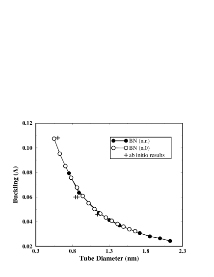
FIG. 2.: Buckling in the BN nanotube equilibrium structures vs. tube diameter. We define the buckling as the mean radius of the nitrogen atoms minus the mean radius of the boron atoms. The ab initio results are from ref. [8].

A structural feature which is specific to the BN nanotubes is the presence of a certain degree of buckling on the tube surface, which results from the B atoms displacing towards the tube axis, while the N atoms displace in the opposite direction. Notice the good agreement with ab initio results [8]. As for the strain energy, the buckling effect decreases rapidly with increasing tube diameter, going to the flat BN sheet limit of zero buckling. This tendency of BN nanotubes to buckle, which is a result of the slightly different hybridizations of B and N in the curved hexagonal layer, will have the effect of forming a surface dipole, a fact that could be relevant for potential applications of these tubes.

In Fig. 3 we have plotted the values of $Y_{s}$ obtained for the different tubes. The first feature to be noticed is the fact that both for (n,n) and (n,0) nanotubes, the carbon tubes are predicted to be significantly stiffer than any of the composite tubes. The $\mbox{BC}_{2}\mbox{N}$ are predicted to be somewhat stiffer than BN and $\mbox{BC}_{3}$ tubes. The value of 0.43 $\mbox{TPa}\cdot\mbox{nm}$ obtained for the widest C nanotubes corresponds to a Young modulus of 1.26 TPa, taking a value of 0.34 nm for the graphene sheet thickness. This value is in excellent agreement with the experimental result of $1.28\pm 0.59$ TPa of Wong et al. [23]. Although our results are only for single-wall tubes, it can be expected that the elastic properties of multi-wall tubes and nanoropes be mostly determined by the strength of the C–C bonds in the bent graphene sheets, and thus be very similar to those of single-wall tubes. Our results for C nanotubes are also in reasonable agreement with the measurements of Treacy et al. [22] ($1.8\pm 1.4$ TPa). Chopra and Zettl [24] obtain a value of 1.22 TPa with an estimated 20 % error for multi-wall BN nanotubes. This value is again somewhat larger than what we obtain for BN nanotubes, but nevertheless, the agreement is close. Lu’s [21] estimation of the Young modulus for single-wall C nanotubes gives results which are slightly smaller than ours (0.97 TPa), a difference which is most likely due to the different models used in his calculations and ours.

Our calculations predict that there is a small dependence of $Y_{s}$ on the tube diameter, but this dependence is noticeable only for small values of the tube diameter, the limiting (diameter independent) value being rapidly obtained at the range of experimentally observed single-wall tube diameters ($\sim 1.2$ nm). This is in contrast to the results of Lu [21], which are almost completely independent of the tube size and chirality. We believe that the apparent insensibility of the Young modulus on the tube size and chirality observed by Lu is due to the fact that an empirical pair potential was used in his calculations, and such a model will not reflect the effects that the curvature will have on the bonding properties of the system. In the limit of large tube diameters, we could expect that the elastic properties would correspond to those of a plane, defect-free, graphitic sheet. Indeed, calculations of $Y_{s}$ for plane graphene and BN sheets give 0.41 and 0.30 $\mbox{TPa}\cdot\mbox{nm}$ respectively, which can be seen to be very similar to the results obtained for C and BN nanotubes of the largest diameter we studied. It is worth noticing that the limiting value of the Young modulus as a function of tube diameter is reached from below, which is consistent with the expectation that tubes of higher curvature (i.e. smaller diameter) will have weaker bonds, which would result in a slight reduction of the Young modulus.

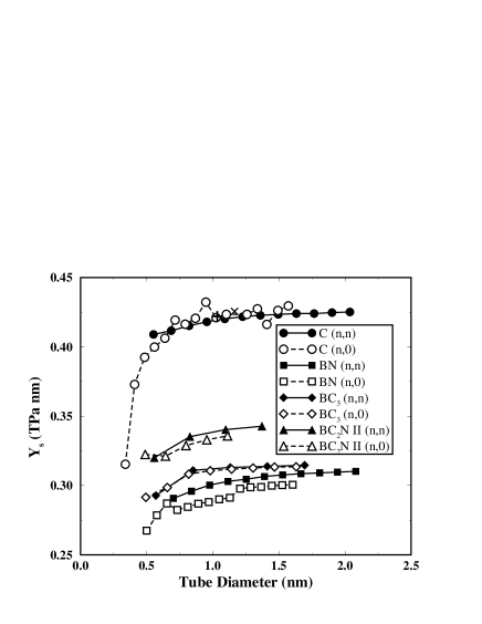
FIG. 3.: Young modulus as a function of the tube diameter for C, BN, $\mbox{BC}_{3}$ and $\mbox{BC}_{2}\mbox{N}$ (structure II only), as calculated from the tight-binding simulations. Results obtained for (n,n) nanotubes (filled symbols), (n,0) nanotubes (empty symbols) and also for C (10,5) ($+$) and (10,7) ($\times$) are shown.

To summarize, we have carried out an extensive study of the energetic, structural and elastic properties of both graphitic and composite nanotubes, using a non-orthogonal Tight-Binding scheme. The agreement obtained between the TB results and the first-principles calculations reassure us in our conclusion that the TB model employed here gives a good description of the studied features of nanotubes. We have obtained good agreement with the existing experimental measurements of the Young modulus for multi-wall C and BN nanotubes. Our results indicate that graphitic nanotubes are stiffer than any of the composite nanotubes considered in this work, and that the elastic properties of single-wall nanotubes are of the same order of magnitude as those of the corresponding flat sheets. Although the BN nanotubes are predicted to have a somewhat smaller Young modulus than the C nanotubes, they remain considerably stiff. This fact, combined with their insulator character [8] makes them suitable for applications in which electrically insulating high-strength materials are needed.

We would like to express our gratitude to G. Seifert and T. Heine for providing the TB parameters used in this work and for helpful discussions concerning implementation details. We are also grateful to P. Bernier and to M. Galtier for stimulating discussions. Financial support was provided by the EU through its Training and Mobility of Researchers Programme under contract ERBFMRX-CT96-0067 (D612-MITH). The use of computer facilities at C4 (Centre de Computació i Comunicacions de Catalunya) and CNUSC (Montpellier) is also acknowledged.

REFERENCES

- [1] See e.g. P.M. Ajayan and T.W. Ebbesen, Rep. Prog. Phys. 60 1025 (1997); M.S. Dresselhaus, G. Dresselhaus and P.C. Eklund, Science of Fullerenes and Carbon Nanotubes (Academic Press, New York 1996).
- [2] S. Iijima, Nature 354 56 (1991); S. Iijima and T. Ichihashi, Nature 363 603 (1993).
- [3] H. Dai et al., Nature 384 147 (1996).
- [4] W.A. de Heer et al., Science 270 1179 (1995); A.G. Rinzler et al., Science 269 1550 (1995).
- [5] P.G. Collins et al., Science 278 100 (1997).
- [6] A.C. Dillon et al., Nature 386 377 (1997).
- [7] A. Rubio, Cond. Matt. News 6 6 (1997).
- [8] A. Rubio, J.L. Corkill and M.L. Cohen, Phys. Rev. B 49 5081 (1994); X. Blase et al. Europhys. Lett. 28 335 (1994); Phys. Rev. B 51 6868 (1995).
- [9] Y. Miyamoto et al., Phys. Rev. B 50 18360 (1994).
- [10] Y. Miyamoto et al., Phys. Rev. B 50 4976 (1994).
- [11] Y. Miyamoto, M.L. Cohen and S.G. Louie, Solid State Comm. 102 605 (1997).
- [12] N.G. Chopra et al., Science 269 966 (1995); A. Loiseau et al. Phys. Rev. Lett. 76 4737 (1996).
- [13] Z. Weng-Sieh et al., Phys. Rev. B 51 11229 (1995).
- [14] K. Suenaga et al., Science 278 653 (1997).
- [15] D.H. Robertson, D.W. Brenner and J.W. Wintmire, Phys. Rev. B 45 12592 (1992).
- [16] R.S. Ruoff and D.C. Lorents, Carbon 33 925 (1995).
- [17] J.M. Molina, S.S. Savinsky and N.V. Khokhriakov, J. Chem. Phys. 104 4652 (1996).
- [18] B.I. Yakobson, C.J. Brabec and J. Bernholc, Phys. Rev. Lett. 76 2411 (1996).
- [19] C.F. Cornwell and L.T. Wille, Solid State Comm. 101 555 (1997).
- [20] S. Iijima et al., J. Chem. Phys. 104 2089 (1996).
- [21] J.P. Lu, Phys. Rev. Lett. 79 1297 (1997).
- [22] M.M.J. Treacy, T.W. Ebbesen and J.M. Gibson, Nature 381 678 (1996).
- [23] E.W. Wong, P.E. Sheehan and C.M. Lieber, Science 277 1971 (1997).
- [24] N.G. Chopra and A. Zettl, Solid State Comm. 105 297 (1998).
- [25] D. Porezag et al., Phys. Rev. B 51 12947 (1995); J. Widany et al. Phys. Rev. B 53 4443 (1996); F. Weich, J. Widany, T. Frauenheim and G. Seifert (private communication).
- [26] For a review on tight-binding see C.M. Goringe, D.R. Bowler and E. Hernández, Rep. Prog. Phys. 60 1447 (1997).
- [27] See e.g. M.C. Payne et al., Rev. Mod. Phys. 64 1045 (1992).
- [28] J. Tersoff, Phys. Rev. Lett. 61 2879 (1988); D.W. Brenner, Phys. Rev. B 42 9458 (1990).
- [29] A.Y. Liu, R.M. Wentzcovitch and M.L. Cohen, Phys. Rev. B 39 1760 (1989).
- [30] N. Troullier and J.L. Martins, Phys. Rev. B 43 1993 (1991).