Numerical Renormalization Group Calculations for the Self-energy of the impurity Anderson model

Abstract

We present a new method to calculate directly the one-particle self-energy of an impurity Anderson model with Wilson’s numerical Renormalization Group method by writing this quantity as the ratio of two correlation functions. This way of calculating $\Sigma(z)$ turns out to be considerably more reliable and accurate than via the impurity Green’s function alone. We show results for the self-energy for the case of a constant coupling between impurity and conduction band ($\Im m\Delta(\omega+i0^{+})\!=\!$ const) and the effective $\Delta(z)$ arising in the Dynamical Mean Field Theory of the Hubbard model. Implications to the problem of the metal-insulator transition in the Hubbard model are also discussed.

¹ Max-Planck-Institut für Physik komplexer Systeme, Nöthnitzer Str. 38, 01187 Dresden, Germany
² Department of Mathematics, Imperial College, 180 Queen’s Gate, London SW7 2BZ, UK
³ Institut für Theoretische Physik der Universität, 93040 Regensburg, Germany

1 Introduction

The single impurity Anderson model [1] is one of the most fundamental and probably the best understood model for strong electronic correlations. Invented to describe the properties of magnetic impurities in non-magnetic metallic hosts 35 years ago, a variety of standard techniques have been applied to it and new methods have been developed to study its static and dynamic properties in basically the whole parameter space (for a review see e.g. [2]). Although a very clear picture of the physics of the single impurity Anderson model has emerged from these calculations, a reliable method for calculating dynamic properties at very low temperatures and intermediate or large values of the Coulomb interaction was for a long time missing.

For example, Bethe ansatz calculations [3], which are essentially exact, can only access static properties and the Quantum Monte Carlo method [4], which can be viewed as another numerically exact technique, cannot reach very low temperatures and/or large values of the Coulomb parameter, although it does not suffer from a minus sign problem here. In addition, the analytic continuation of the imaginary time data to real frequencies is a numerically highly ill-conditioned problem.

Among the approximate treatments the resolvent perturbation theory together with the so-called Non-Crossing Approximation [5] turned out to be a simple and powerful technique for high and intermediate temperatures of the order of the Kondo scale but completely fails to reproduce the local Fermi-liquid properties as $T\!\to\!0$. Last but not least, straightforward second-order perturbation theory in $U$ [6] has been shown to work surprisingly well down to $T\!=\!0$ but it is restricted to the symmetric case and not too large values of $U$.

The Numerical Renormalization Group method (NRG), invented by Wilson for the Kondo problem [7] and later applied by Krishnamurthy et al. to the impurity Anderson model [8], is usually acknowledged primarily in the context of universality and low-energy fixed point behaviour of the Kondo or Anderson model. One of its most appealing features is that it can deal equally well with small, intermediate or large values of $U$ and is not restricted to half-filling. During the last 15 years considerable progress has been made to extract dynamical properties with this method, too, and it has been shown to give very accurate results also for e.g. dynamical one- and two-particle and also transport properties [9, 10]. The NRG works best at $T\!=\!0$, and various dynamic correlation functions can be calculated with an accuracy of a few percent. Although less well defined for finite temperatures, its extension to $T\!>\!0$ also shows very good agreement with exact results [10]. It is quite remarkable that no sum-rules (Friedel sum rule, total spectral weight) must be used as input for these calculations. On the contrary, they can serve as an independent check on the quality of the results.

More recent interest in reliable methods to solve the impurity Anderson model and calculate its dynamical properties has been motivated by the discovery that lattice models in the limit of infinite dimensions acquire a purely local one particle self-energy [11]. This simplification eventually leads to a mapping of the lattice problem on an effective impurity Anderson model coupled to a medium to be determined self-consistently [12]. Note that in the general case the solution of this self-consistency requires the knowledge of the one particle self-energy. In view of the wide range of problems to which this so-called Dynamical Mean Field Theory (DMFT, see e.g. [13]) can be applied, it seems surprising why there have been hardly any contributions using the NRG. The only NRG-calculation known to us is the work of Sakai et al. [14] where the symmetric Hubbard model in the metallic regime was studied. In their paper, these authors point out some difficulties in the progress of iterating the NRG results with the DMFT equations, which are largely related to the necessary broadening of the NRG spectra (see further below).

In this contribution we present a new method to calculate dynamic properties for the impurity Anderson model, namely by directly constructing the interaction contribution to the self-energy as the ratio of two correlation functions, $\Sigma^{U}_{\sigma}(z)\!=\!UF_{\sigma}(z)/G_{\sigma}(z)$, with $F_{\sigma}(z)\!=\langle\!\langle f_{\sigma}f^{\dagger}_{\bar{\sigma}}f_{\bar{\sigma}},f^{\dagger}_{\sigma}\rangle\!\rangle_{z}$ and $G_{\sigma}(z)\!=\langle\!\langle f_{\sigma},f^{\dagger}_{\sigma}\rangle\!\rangle_{z}$ (see Section II). Details of how to calculate the $F(z)$ are given in the appendix. In section III we discuss results for

• the standard case, where the coupling between impurity states and metallic host, $\Im m\Delta(\omega+i0^{+})$, is constant,

• and the Hubbard model in $d\!=\!\infty$, where $\Delta(z)$ has to be determined self-consistently.

The Hubbard model is studied in the paramagnetic regime, at half-filling and $T\!=\!0$. We discuss the properties of self-energy and local density of states both in the metallic and insulating regimes and some preliminary results for the metal-insulator transition.

2 Calculation of the self-energy

Model and basic concepts

The impurity Anderson model is written in the form

$$H = \sum_{\sigma}\varepsilon_{\rm f}f^{\dagger}_{\sigma}f_{\sigma}+Uf^{\dagger}_{\uparrow}f_{\uparrow}f^{\dagger}_{\downarrow}f_{\downarrow}$$ (1)

$$+ \sum_{k\sigma}\varepsilon_{k}c^{\dagger}_{k\sigma}c_{k\sigma}+\sum_{k\sigma}V_{k}\Big{(}f^{\dagger}_{\sigma}c_{k\sigma}+c^{\dagger}_{k\sigma}f_{\sigma}\Big{)}.$$

In the model (1), $c_{k\sigma}^{(\dagger)}$ denote standard annihilation (creation) operators for band states with spin $\sigma$ and energy $\varepsilon_{k}$, $f_{\sigma}^{(\dagger)}$ those for impurity states with spin $\sigma$ and energy $\varepsilon_{\rm f}$. The Coulomb interaction for two electrons at the impurity site is given by $U$ and both subsystems are coupled via a hybridization $V_{k}$, which we allow to be $k$-dependent here.

Our final goal is to calculate the one-particle Green’s function $G_{\sigma}(z)=\langle\!\langle f_{\sigma},f^{\dagger}_{\sigma}\rangle\!\rangle_{z}$, which formally can be written as

$$G_{\sigma}(z)=\frac{1}{z-\varepsilon_{\rm f}-\Sigma_{\sigma}(z)}\;\;.$$ (2)

While this formal introduction of the one particle self-energy $\Sigma(z)$ is straight forward, the actual calculation of $G(z)$ or alternatively $\Sigma(z)$ usually is an extremely complicated problem. In order to express the self-energy $\Sigma(z)$ by standard impurity correlation functions, we make use of the equation of motion

$$z\langle\!\langle A,B\rangle\!\rangle_{z}+\langle\!\langle{\cal L}A,B\rangle\!\rangle_{z}=\langle[A,B]_{\eta}\rangle,$$ (3)

with ${\cal L}\cdot\equiv[H,\cdot]_{-}$ and $\eta=+$, if both $A$ and $B$ are fermionic operators, $\eta=-$ otherwise. The correlation functions are defined as $\langle\!\langle A,B\rangle\!\rangle_{z}\!=\!i\int_{0}^{\infty}e^{izt}\langle[A(t),B]_{\eta}\rangle$. For $A=f_{\sigma}$ and $B=f^{\dagger}_{\sigma}$ we obtain the equation of motion for the f-Green’s function as

$$(z-\varepsilon_{\rm f})G_{\sigma}(z)-U\langle\!\langle f_{\sigma}f^{\dagger}_{\bar{\sigma}}f_{\bar{\sigma}},f^{\dagger}_{\sigma}\rangle\!\rangle_{z}-\sum_{k}V_{k}\langle\!\langle c_{k\sigma},f^{\dagger}_{\sigma}\rangle\!\rangle_{z}=1\ .$$

The correlation function $\langle\!\langle c_{k\sigma},f^{\dagger}_{\sigma}\rangle\!\rangle_{z}$ is related to $G_{\sigma}(z)$ via eq. (3) with $A=c_{k\sigma}$ and $B=f^{\dagger}_{\sigma}$ through

$$(z-\varepsilon_{k})\langle\!\langle c_{k\sigma},f^{\dagger}_{\sigma}\rangle\!\rangle_{z}-V_{k}G_{\sigma}(z)=0\ .$$ (4)

The $U$-term does not enter this equation as the Coulomb interaction only acts on the impurity states. Together with (4) eq. (2) has the form

$$(z-\varepsilon_{\rm f})G_{\sigma}(z)-UF_{\sigma}(z)-\Delta(z)G_{\sigma}(z)=1,$$ (5)

where we have defined $F_{\sigma}(z)=\langle\!\langle f_{\sigma}f^{\dagger}_{\bar{\sigma}}f_{\bar{\sigma}},f^{\dagger}_{\sigma}\rangle\!\rangle_{z}$ and $\Delta(z)=\sum_{k}V_{k}^{2}\frac{1}{z-\varepsilon_{k}}$. The total self-energy $\Sigma_{\sigma}(z)$ for the single impurity Anderson model is thus given by

$$\Sigma_{\sigma}(z)=\Delta(z)+\Sigma_{\sigma}^{U}(z)\;\;,$$ (6)

where the nontrivial part due to the Coulomb correlations $\Sigma^{U}(z)$ is obtained from

$$\Sigma^{U}_{\sigma}(z)=U\frac{F_{\sigma}(z)}{G_{\sigma}(z)},$$ (7)

For simplicity and since we are only interested in the paramagnetic situation for the time being the spin index will be dropped in the following.

Alternatively, the interaction part of the self-energy can of course also be calculated directly from eq. (2) using

$$\Sigma^{U}(z)=G_{0}(z)^{-1}-G(z)^{-1},\ \ {\rm with}\ \ G_{0}(z)=\frac{1}{z-\varepsilon_{\rm f}-\Delta(z)}.$$ (8)

On a first glance, there seems to be no apparent reason to prefer the more complicated equation (7) over equation (8). In order to clarify the advantage of using eq. (7) instead of eq. (8) for the calculation of $\Sigma^{U}(z)$ with the NRG we want to give a brief description of how the spectral densities for $G(z)$ and $F(z)$ are calculated with the NRG.

Technical details

Within the NRG, the impurity Anderson model eq. (1) is mapped onto a semi-infinite chain (see [7, 8]) which is diagonalized iteratively starting from the uncoupled impurity. At each iteration, the number of states increases by a factor of 4 and after a certain number of iterations, the basis kept for the next iteration has to be truncated. The important point of the method is that the coupling between consecutive elements of the chain decreases exponentially for increasing distance from the origin, so that with increasing chain length at each iteration basically only the lowest lying states will be renormalized and such a truncation is meaningful. The spectral functions at each iteration are calculated from the corresponding matrix elements, which are in turn related to those of the previous iteration. This procedure is well established for the one-particle density of states $A(\omega)=-\frac{1}{\pi}\Im mG(\omega+i0^{+})$ [9, 10] and can straight forwardly be extended to $B(\omega)=-\frac{1}{\pi}\Im mF(\omega+i0^{+})$. For details we refer the reader to the appendix. Due to the truncation of states, the spectral function for the whole frequency range has to be built up from the data of all the iterations.

The resulting spectral function is a set of $\delta$-functions at frequencies $\omega_{n}$ with weights $g_{n}$ which are broadened on a logarithmic scale as

$$g_{n}\delta(\omega-\omega_{n})\longrightarrow g_{n}\frac{e^{-b_{n}^{2}/4}}{b_{n}\omega_{n}\sqrt{\pi}}\exp\left[-\frac{(\ln\omega-\ln\omega_{n})^{2}}{b_{n}^{2}}\right].$$ (9)

This form of broadening was also used in [9] and [10] and is especially adapted to the exponential variation in energies peculiar to the NRG. The width $b_{n}$ is chosen as $b$ independent of $n$ and we use values $0.3\leq b\leq 0.6$.

It is well known that with this scheme the NRG gives already quite accurate results for $G(z)$ [9, 10]. However, one might anticipate some problems with the calculation of $\Sigma^{U}(z)$ using eq. (8). The function $G_{0}(z)^{-1}$ is, of course, known exactly since $\Delta(z)$ is a given quantity. Building the difference between an exactly known and a numerically determined function is usually very susceptible to numerical errors, especially in regions where the result becomes small. Since this is expected to happen close to the Fermi level, i.e. in the physically most relevant region, one is likely to run into problems there.

One naive attempt to reduce these kind of inconsistencies and numerical errors when building the difference in eq. (8) is to treat $G_{0}(z)^{-1}$ and $G(z)^{-1}$ on the same level, that is to calculate $G_{0}(z)^{-1}$ via the NRG as well by setting $U=0$. However, since according to the theory of error propagation in sums or differences the absolute errors add, one must expect this procedure to be also ill-conditioned. If both $G_{0}(z)$ and $G(z)$ are known exactly, the difference $G_{0}(z)^{-1}\!-\!G(z)^{-1}$ always gives a negative imaginary part for the self-energy as there would be a pole in $G(z)^{-1}$ for every pole in $G_{0}(z)^{-1}$ at the same energy with equal or larger residue. This is no longer guaranteed as soon as both $G_{0}(z)$ and $G(z)$ are only known approximately, and one has to use rather large values of the broadening parameter $b$ to avoid unphysical oscillations in $\Sigma^{U}(z)$. This broadening in turn leads to a strong suppression of the high energy peaks because spectral weight is shifted from the center of the peak to its tails (to the high energy side due to eq.  (9)).

For the calculation of $\Sigma^{U}(z)$ via eq. (7) on the other hand we do not expect to face these kind of problems that severely. Again, both quantities are calculated on the same basis by broadening the NRG results with (9), i.e. with the same systematic error. This time, however, we divide them by each other, which means that only the relative errors will be propagated, leading to a numerically much more stable procedure.

Let us support this rather qualitative argument in favour of expressing the self-energy as the ratio $UF(z)/G(z)$ by comparing the spectral function $\bar{A}(\omega)$ obtained directly from the NRG (solid line in Fig. 1) and the ${A}(\omega)$ calculated from eq. (2) with the self-energy expressed as in eq. (7) (dashed line in Fig. 1). The spectral functions are defined as ${A}(\omega)=-\frac{1}{\pi}\Im mG(\omega+i0^{+})$. The parameters are $\varepsilon_{\rm f}\!=\!-0.1D$, $U\!=\!0.2D$ and $-\Im m\Delta(\omega+i0^{+})\!=\!\Delta_{0}\!=\!0.015D$, where $2D$ is the conduction electron bandwidth. For convenience we use $D\!=\!1$ as energy scale for the rest of the paper.

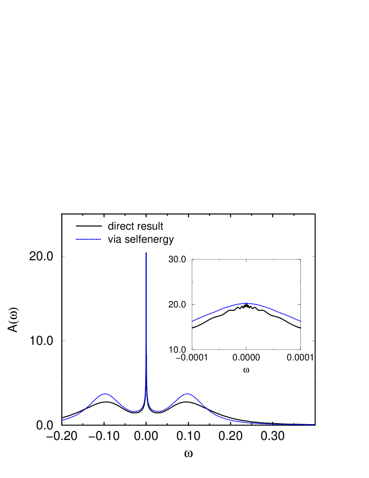
Figure 1: Impurity spectral function for $\varepsilon_{\rm f}\!=\!-0.1$, $U\!=\!0.2$, $T\!=\!0$ and $-\Im m\Delta(\omega+i0^{+})=0.015$ in units of the conduction electron band width. $\bar{A}(\omega)$ (solid line) is the result obtained directly from the NRG and ${A}(\omega)$ (dashed line) is calculated via the self-energy eq. (7). The inset shows the region around the Fermi-level.

The differences between the two methods can be summarized as follows:

• We find for the total spectral weight $\int d\omega\bar{A}(\omega)\!=\!\bar{w}\!=\!0.93$ and $\int d\omega{A}(\omega)\!=\!{w}\!=\!0.9993$. The 7% deviation in $\bar{w}$ can in principle be reduced by improving the resolution of the NRG calculation (smaller deviations have been achieved e.g. in [9, 10]). This is, however, not necessary in our case because the self-energy resulting from eq. (7) is an analytic function and the sum-rule $w\!=\!1$ is then automatically fulfilled (apart from the very small numerical error).

• The charge fluctuation peaks near $\varepsilon_{\rm f}$ are much more pronounced in $A(\omega)$. That the high energy features are usually underrated is a well-known problem in the calculation of dynamical properties with the NRG. This problem is at least partially resolved in our new scheme, since the main contribution in this part of the spectrum rather comes from the hybridization part $\Delta(z)$, which is treated exactly.

• The oscillations in $\bar{A}(\omega)$ near $\omega\!=\!0$ are due to the choice of the broadening which is obviously too small to see the correct low-frequency behaviour of the spectral function. These oscillations almost vanish in ${A}(\omega)$ and the $\omega^{2}$- behaviour can be clearly identified.

• The deviation from the Friedel sum-rule

  $$A(0)=-\frac{1}{\pi\Im m\Delta(i0^{+})}=:\frac{1}{\pi\Delta_{0}},$$ (10)

  ($\approx 21$ for the parameters used here) is about 7% in $\bar{A}(\omega)$ and 4% in ${A}(\omega)$.

Although the error in the Friedel sum-rule is visibly reduced, the deviation is still a few percent. Its origin will be discussed in the following.

Numerical aspects

It is important to understand the origin of the deviation of $A(0)$ (Friedel sum-rule) from its exact value as this lies at the heart of the numerical procedure.

Typical results for $A(\omega)$ and $B(\omega)$ as calculated with the NRG

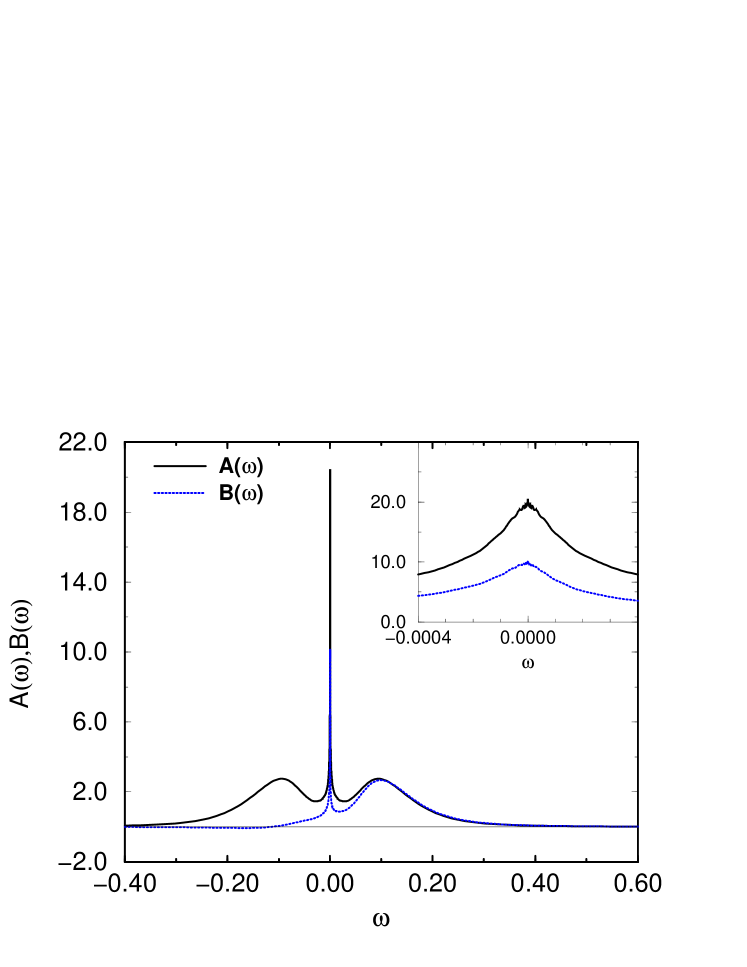
Figure 2: Spectral functions $A(\omega)$ (solid line) and $B(\omega)$ (dotted line) for the same parameters as in Fig. 1 (directly from the NRG, not via the self-energy). The inset shows the region around the Fermi-level.

are shown in figure 2. Both spectral functions $A(\omega)$ and $B(\omega)$ display a sharp resonance close to the Fermi energy. However, in contrast to $A(\omega)$, which is positive definite and perfectly symmetric to $\omega=0$ due to the particle-hole symmetry, the function $B(\omega)$ is obviously not positive definite and appears to be extremely asymmetric.

As next step we must calculate the real parts, which are obtained via standard Kramers-Kronig transformation. The self-energy finally is given with eq. (7) as

$${\Re e}\Sigma^{U}(\omega+i0^{+})+i{\Im m}\Sigma^{U}(\omega+i0^{+})=U\frac{{\Re e}F(\omega+i0^{+})+i{\Im m}F(\omega+i0^{+})}{{\Re e}G(\omega+i0^{+})+i{\Im m}G(\omega+i0^{+})}.$$ (11)

In the particle-hole symmetric case, $\Re eG(\omega+i0^{+})$ necessarily vanishes at $\omega\!=\!0$, therefore

$${\Re e}\Sigma^{U}(0^{+})=U\frac{{\Im m}F(i0^{+})}{{\Im m}G(i0^{+})},$$ (12)

which of course has to give the Hartree term $U/2$, and

$${\Im m}\Sigma^{U}(i0^{+})=-U\frac{{\Re e}F(i0^{+})}{{\Im m}G(i0^{+})}.$$ (13)

In the case of the standard single-impurity Anderson model we furthermore know that the Friedel sum-rule ${\Im m}\Sigma^{U}(i0^{+})=0$ has to be fulfilled, which implies that

$$\Re eF(i0^{+})=-\int\limits_{-\infty}^{\infty}d\omega B(\omega){\cal P}\frac{1}{\omega}=0\;\;,$$ (14)

where ${\cal P}(\ldots)$ denotes the principal value. The relation (14) is obviously not trivial regarding the unusual shape of $B(\omega)$. It indeed turns out that $\Re eF(i0^{+})$ is numerically zero as long as the full spectrum of the Hamiltonian can be used. However, as soon as a truncation of states sets in the calculated value for $\Re eF(i0^{+})$ suddenly jumps to a finite value, eventually leading to a violation of the Friedel sum-rule as observed e.g. in Figure 1.

This observation suggests that also high energy states are important to guarantee that $\Re eF(i0^{+})\!=\!0$ and that a slight violation of the Friedel sum-rule is almost unavoidable in this method.

3 Results

Single impurity Anderson model

As a simple example let us discuss the standard case of a constant $\Im m\Delta(\omega+i0^{+})$,

$$-\Im m\Delta(\omega+i0^{+})=\left\{\begin{array}[]{lcl}\Delta_{0}&:&|\omega|<1\\ 0&:&|\omega|>1\end{array}\right..$$ (15)

Figure 3: Real and imaginary part of the self-energy for $\varepsilon_{\rm f}\!=\!-0.1$, $U\!=\!0.2$, and a constant $\Delta_{0}\!=\!0.015$. The inset shows the region around the Fermi level where the Hartree term was subtracted off the real part.

The application of the NRG to this model has been discussed very extensively in the literature [9, 10]. Thus the results presented here surely give no new insight into the physics of this model. They are mainly intended to give the reader a feeling for the quality of our method.

Figure 3 shows the results for the real and imaginary part of $\Sigma^{U}(z)$ for $\varepsilon_{\rm f}\!=\!-0.1$, $U\!=\!0.2$, $\Delta_{0}\!=\!0.015$ and $T\!=\!0$. As a first important point we note that the real part of the self-energy has a constant contribution. If we calculate $\Re e\Sigma^{U}(\omega)+\Re e\Sigma^{U}(-\omega)$, we obtain the expected value U/2 to within numerical precision for all $\omega$. This result also shows that, although $B(\omega)$ is asymmetric, the final result obeys the particle-hole symmetry to a high precision. In addition the slope $\left.\partial\Re e\Sigma^{U}(\omega)/\partial\omega\right|_{\omega=0}$ is negative and large, corresponding to a high effective mass.

The imaginary part of $\Sigma^{U}(z)$ shows two pronounced peaks at $\omega\!\approx\!\pm 0.03$ and a steep decrease as $\omega\to 0$. In the vicintiy of the Fermi level we find the Fermi liquid property $\Im m\Sigma^{U}(\omega+i0^{+})\!\propto\!\omega^{2}$ (inset of Figure 3). However, as pointed out in the previous section, the Friedel sum rule $\Im m\Sigma^{U}(i0^{+})=0$ is not exactly fulfilled. The shift of $\Im m\Sigma^{U}(i0^{+})\!\approx-0.0007$ corresponds to a 4% error in $A(0)\!=\!1/(\pi\Delta_{0})$.

Figure 4 finally shows the resulting spectral function for various values of $U$.

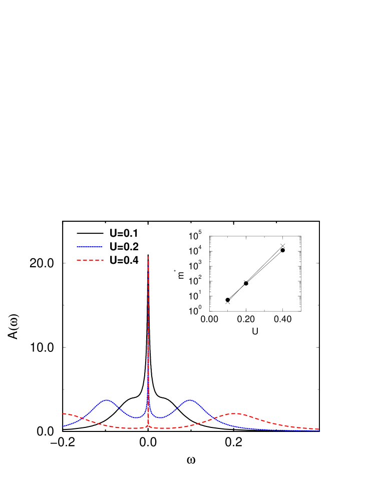
Figure 4: Spectral function for $\varepsilon_{\rm f}\!=\!-U/2$, $\Delta_{0}\!=\!0.015$ and various values of $U$. The inset shows the resulting effective mass $m^{\ast}$ (filled circles) together with the expected behaviour $m^{\ast}\propto\sqrt{U}\exp(\pi U/(8\Delta_{0}))$ (crosses).

As mentioned previously in section 2, we find pronounced charge fluctuation peaks at $\pm U/2$ and the characteristic Abrikosov-Suhl resonance at the Fermi level. With increasing $U$ this resonance becomes sharper. The corresponding energy scale expressed via the effective mass is shown in the inset to figure 4 together with the expected behaviour $m^{\ast}\propto\sqrt{U}\exp(\pi U/(8\Delta_{0}))$.

Application to the Hubbard model

The impurity Anderson model is not only useful to describe magnetic impurities in nonmagnetic metals. It was shown only recently that in the limit of infinite spatial dimensions a lattice model (Hubbard model, Periodic Anderson Model, etc.) with local interactions can be mapped on an effective single impurity Anderson model. The quantity $\Delta(z)$, which in the single impurity model describes the coupling to the metallic host, becomes in general an energy dependent quantity here, which has a meaning similar to the Weiss field in the mean-field theory of the Heisenberg model. Since $\Delta(z)$ is a dynamic quantity which must be determined self-consistently as functional of the one-particle self-energy [11, 12, 13], the name “Dynamical Mean Field Theory” (DMFT) has been coined.

This self-consistency makes it necessary to calculate the self-energy $\Sigma^{U}(z)$ as accurate as possible. Here we want to demonstrate that the NRG together with the method of calculating $\Sigma^{U}(z)$ presented in the previous section is indeed a reliable and accurate method to do this job at $T=0$.

The first step in order to apply the NRG is the mapping of the impurity model on a semi-infinite chain for the case of a non-constant $\Im m\Delta(\omega+i0^{+})$ which we have already described in [15]. As the resulting $\Im m\Delta(\omega+i0^{+})$ can develop very narrow structures at the Fermi level, we need a reliable numerical method to calculate $\approx$ 60 - 100 hopping matrix elements of the chain. This is done using arbitrary-precision fortran routines. Apart from the difference in the hopping matrix elements, the calculation of $F(z)$, $G(z)$ and $\Sigma^{U}(z)$ follows the same procedure as in the flat-band case.

The simplest model for correlation effects in solids is the well-known Hubbard model [16]. This model is believed to have a rich phase diagram despite its comparatively simple form. DMFT studies at finite temperatures indeed revealed for example antiferromagnetic [17, 13] and ferromagnetic transitions [18, 19], Mott-Hubbard metal insulator transition [13] etc. . Nevertheless, there still remain lots of interesting open questions, especially about the properties of the model at extremely low temperatures both at and away from half filling.

Here we study the Hubbard model at $T=0$ for a semi-circular density of states $\rho_{0}(\varepsilon)$ corresponding to the Bethe lattice with infinite coordination number

$$\rho_{0}(\varepsilon)=\frac{2}{\pi}\sqrt{1-\varepsilon^{2}},$$ (16)

($D\!=\!1$) at particle-hole symmetry and in the paramagnetic regime. The resulting spectral functions for the paramagnetic Hubbard model for various values of $U$ are collected in Figure 5.

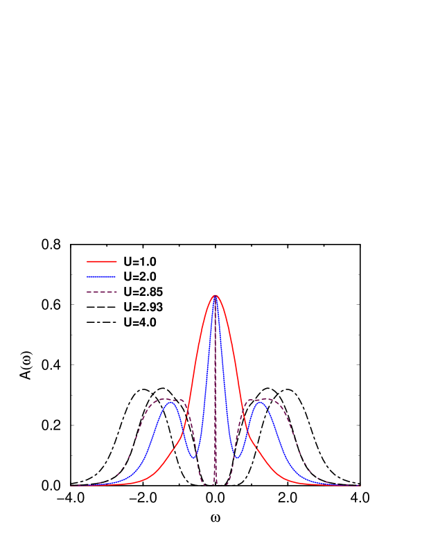
Figure 5: Local spectral function of the Hubbard model for various values of $U$. A quasiparticle peak develops for increasing values of $U$ which vanishes at a critical value $U_{\rm c}\!\approx\!2.93$, signalling the metal-insulator transition.

With increasing $U$, the one-particle spectrum develops the typical three-peak structure with a quasiparticle peak at $\omega\!=\!0$ and the two Hubbard bands at $\pm U/2$. Above a certain value $U_{\rm c}\approx 2.93$ the central peak vanishes and the system becomes insulating.

Figure 6 and 7 show the real and imaginary part of the self-energy for the same parameters as in Fig. 5 ($U\!=\!1$ and $U\!=\!4$ are not shown). The Hartree term in the real part ($=\!U/2$) is subtracted. The negative slope at the Fermi level diverges as $U\to U_{\rm c}$. For $U\!\geq\!2.93$ (the insulating solution) the real part shows a $1/\omega$-divergence. The corresponding $\delta$-peak in the imaginary part is not plotted in Fig. 7. This $\delta$-peak in Im$\Sigma^{U}(\omega)$ emerges from a two-peak structure in the metallic regime, with the positions of the two peaks approaching $\omega\!=\!0$ for $U\to U_{\rm c}$. The imaginary part shows the Fermi liquid behaviour Im$\Sigma^{U}(\omega)\propto\omega^{2}$ at low frequencies for $U<U_{\rm c}$

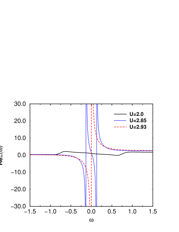
Figure 6: Real part of the self-energy for the Hubbard model (same parameters as in Fig. 5). The negative slope at $\omega\!=\!0$ diverges at the metal-insulator transition. For $U\!\geq\!U_{\rm c}$, the real part shows a $1/\omega$-divergence.

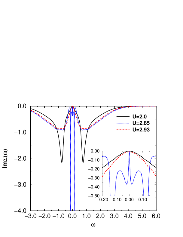
Figure 7: Imaginary part of the self-energy for the Hubbard model (same parameters as in Fig. 5). A $\delta$-function develops for $U\to U_{\rm c}$.

In order to give the reader an idea of the complex structures arising in lattice models, we show in figure 8 a comparison of the NRG flow diagram for the energy levels for the single impurity Anderson model with flat $\Im m\Delta(\omega)$ (figure 8a) and typical results for the Hubbard model in the paramagnetic metallic phase (figure 8b) and paramagnetic insulating phase (figure 8c). In contrast to the single impurity case the flow diagrams for the Hubbard model show a complicated crossover behaviour for high energies (low NRG iteration number) before they saturate into a fixed-point spectrum for large NRG iteration numbers, i.e. low energies. While these fixed-point spectra for the impurity model and the metallic solution of the Hubbard model (figures 8a and b) are identical, i.e. both are Fermi liquids, the fixed point spectrum for the insulator (figure 8c) has a quite different structure (see eg. the flow of the first excited state with $Q\!=\!1,S\!=\!0$ in figure 8b and figure 8c, $Q$ is defined as the particle number with respect to half-filling). In addition the behaviour of the hopping matrix elements for the three cases is shown in figure 8d (diamonds, circles and crosses, respectively). Note the oscillatory behaviour in the latter case characteristic for a system with a pseudogap.

Figure 8: Flow diagrams for the lowest energy levels $E_{Q,S}$ as function of the NRG-iterations $N$. The solid lines correspond to quantum numbers $Q\!=\!0,S\!=\!1/2$ and the dashed lines to quantum numbers $Q\!=\!1,S\!=\!0$. (a) The flat-band case with $\varepsilon_{\rm f}\!=\!-0.2$, $U\!=\!0.4$, and a constant $\Delta_{0}\!=\!0.015$. For large $N$, the system flows to the Fermi liquid fixed point, while in the intermediate regime ($N\approx 20$) it is near the so-called local moment fixed point. (b) The Hubbard model with $U=2$ flows to the same Fermi liquid fixed point as in the flat band case. (c) The Hubbard model with $U=4$ flows to the local moment fixed point corresponding to the insulating behaviour. (d) The hopping matrix elements $t_{N}$ of the semi-infinite NRG chain for Fig. 8a (diamonds), Fig. 8b (circles) and Fig. 8c (crosses), respectively.

The data shown here are quite similar to those obtained by Georges et al. [13] in that the quasiparticle peak seems to be isolated from the two Hubbard bands near $U_{\rm c}$. However, we always find finite spectral weight in the region between the quasiparticle peak and the Hubbard bands. For $U\geq U_{\rm c}$ the quasiparticle peak vanishes but we do not see a real gap, i.e. a region with exactly vanishing density of states. The fact that there is no gap even above the metal-insulator transition is also visible in $\Im m\Sigma^{U}(\omega)$, as there is no region with vanishing $\Im m\Sigma^{U}(\omega)$. The strong suppression of the spectral density between the Hubbard bands and the quasiparticle peak for $U\!=\!2.85$ mainly comes from the large values of $\Re e\Sigma^{U}(\omega)$. The question, whether a real gap will eventually emerge for higher values of $U$ is currently investigated and a more detailed analysis of the metal-insulator transition at $T=0$ will be presented in a subsequent publication.

For the time being we define the point where the transition from a metal to an insulator takes place by the divergence of the effective mass

$$m^{\ast}=1-\left.\frac{\partial}{\partial\omega}{\Re e}\Sigma^{U}(\omega)\right|_{\omega=0}$$ (17)

of the quasi-particles. Note that this scenario completely neglects the possibility of a discontinuous transition for a $U<U_{\rm c}$.

The behaviour of the effective mass as function of $U$ is collected in figure 9. $m^{\ast}$ diverges at $U_{\rm c}\!\approx\!2.93$ and the critical behaviour close to $U_{\rm c}$ is consistent with a powerlaw with an exponent of $\approx-2$. Unfortunately, the data currently available do not allow a precise evaluation of this exponent. Note that our value for $U_{\rm c}$ is considerably smaller than the value of $U_{\rm c,2}\!=\!3.3$ mentioned in the work of Georges et al. [13].

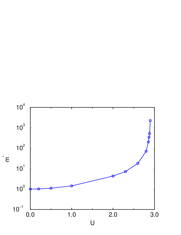
Figure 9: $U$-dependence of the effective mass $m^{\ast}$ for the Hubbard model. $m^{\ast}$ diverges at $U_{\rm c}\!\approx\!2.93$ which defines the critical value of the metal-insulator transition.

4 Summary

In this paper we have presented a new method of calculating the self-energy of the single impurity Anderson model with the Numerical Renormalization Group method. In contrast to the standard approach where one calculates the self-energy from the Green’s function alone, we express $\Sigma^{U}(z)$ as a ratio of two correlation functions. The central aspect of this paper is that this method is much more accurate than the usual method.

The importance of this gain in accuracy goes beyond the mere improvement of the results for the single impurity Anderson model. Our method now in addition allows to apply the NRG to various lattice models within the Dynamical Mean Field Theory, where the self-energy of an effective impurity Anderson model has to be calculated self-consistently. As examples we recapitulated typical results for the single impurity Anderson model and presented results for the Hubbard model with a semi-circular density of states (corresponding to the Bethe lattice with infinite coordination number) at particle-hole symmetry and $T\!=\!0$.

As an interesting but not yet fully confirmed result in the latter case we find that the metal-insulator transition in this model appears more like a metal-semimetal transition, as there is no region in the spectrum where the spectral density exactly vanishes. We defined the critical $U$ via the divergence of the effective mass and found a value $U_{\rm c}\approx 2.93$.

A more detailed analysis of the metal-insulator transition, results for the Hubbard model away from particle-hole symmetry and the investigation of more complicated models (Periodic Anderson model, three-band Hubbard model, etc.) will be discussed in forthcoming publications.

We wish to thank T. Costi, J. Keller and D. Logan for a number of stimulating discussions. One of us (R.B.) was supported by a grant from the Deutsche Forschungsgemeinschaft, grant No. Bu965-1/1. We are also grateful to the EPSRC for the support of a research grant (No. GR/J85349).

Appendix A The correlation function $F(z)$

Here we present some details of the calculation of $F(z)$ and discuss some of its properties.

The NRG uses a discretized version of the Anderson model in a semi-infinite chain form (for details see [7, 8]). The resulting spectral functions will therefore be given as a set of discrete $\delta$-peaks.

The spectral representation of $F(z)$ is

$$B(\omega) = \frac{1}{Z}\sum_{nm}<n|f_{\downarrow}f^{\dagger}_{\uparrow}f_{\uparrow}|m><m|f^{\dagger}_{\downarrow}|n>$$ (18)

$$\times\delta\left(\omega-(E_{m}-E_{n})\right)\left(e^{-\beta E_{n}}+e^{-\beta E_{m}}\right).$$

The matrix elements $<n|f_{\downarrow}f^{\dagger}_{\uparrow}f_{\uparrow}|m>$, $<m|f^{\dagger}_{\downarrow}|n>$ and the energies $E_{n},E_{m}$ are calculated iteratively in the NRG. The two operators

$$V^{1/2}_{1/2} = f_{\downarrow}f^{\dagger}_{\uparrow}f_{\uparrow},$$

$$V^{1/2}_{-1/2} = -f_{\uparrow}f^{\dagger}_{\downarrow}f_{\downarrow},$$ (19)

transform as

$$\left[s^{\pm},V^{1/2}_{q}\right]_{-} = \sqrt{\frac{3}{4}-q(q\pm 1)}\ \ V^{1/2}_{q\pm 1},$$

$$\left[s_{z},V^{1/2}_{q}\right]_{-} = qV^{1/2}_{q},$$ (20)

($q=\pm 1/2$), with the spin operators

$$s^{+}=f^{\dagger}_{\uparrow}f_{\downarrow},\quad s^{-}=f^{\dagger}_{\downarrow}f_{\uparrow},$$

$$s_{z}=\frac{1}{2}\left(f^{\dagger}_{\uparrow}f_{\uparrow}-f^{\dagger}_{\downarrow}f_{\downarrow}\right).$$ (21)

This allows us to use the Wigner-Eckart Theorem

$$\left<Q,S,S_{z},w\right|V^{1/2}_{q}\left|Q^{\prime},S^{\prime},S_{z}^{\prime},w^{\prime}\right>=\big{<}Q,S,w\big{|}\!\big{|}V_{q}^{1/2}\big{|}\!\big{|}Q^{\prime},S^{\prime},w^{\prime}\big{>}\big{<}S^{\prime},S_{z}^{\prime},\frac{1}{2},q|S,S_{z}\big{>}.$$ (22)

The $\big{<}Q,S,w\big{|}\!\big{|}V_{q}^{1/2}\big{|}\!\big{|}Q^{\prime},S^{\prime},w^{\prime}\big{>}$ are reduced matrix elements and the $\big{<}S^{\prime},S_{z}^{\prime},\frac{1}{2},q|S,S_{z}\big{>}$ Clebsch-Gordan coefficients. It is important to note that the operators $V_{q}^{1/2}$ transform in exactly the same way as the two operators

$$W^{1/2}_{1/2} = f^{\dagger}_{\uparrow},$$

$$W^{1/2}_{-1/2} = f^{\dagger}_{\downarrow}.$$ (23)

This has the consequence that all the recursion formulas for the reduced matrix elements of $W^{1/2}_{q}$ can be used for the calculation of the reduced matrix elements of $V^{1/2}_{q}$. The only changes are in the particle numbers $Q$ of the states involved and the initial values (see below).

The states $|n\!>$ and $|m\!>$ in eq. (18) are classified in terms of charge $Q$ (the total particle number relative to the half-filled case), total spin $S$, $z$-component of the total spin $S_{z}$ and an additional label $w$

$$|n> = |Q_{n},S_{n},S_{z,n},w_{n}>,$$

$$|m> = |Q_{m},S_{m},S_{z,m},w_{m}>\ .$$ (24)

The sum over $S_{z,n}$ and $S_{z,m}$ in eq. (18) can be performed exactly and we find

$$B(\omega) = \frac{1}{Z}\sum_{\begin{array}[]{c}{\scriptscriptstyle Q,S,w_{n}}\\ {\scriptscriptstyle S_{m}=S\pm\frac{1}{2},w_{m}}\end{array}}\big{<}Q,S,w_{n}\big{|}\!\big{|}V_{1/2}^{1/2}\big{|}\!\big{|}Q+1,S_{m},w_{m}\big{>}$$

$$\times \big{<}Q+1,S_{m},w_{m}\big{|}\!\big{|}f_{\downarrow}^{\dagger}\big{|}\!\big{|}Q,S,w_{n}\big{>}\delta\left(\omega-(E_{m}-E_{g})\right)$$

$$\times \left(e^{-\beta E_{n}}+e^{-\beta E_{m}}\right)\frac{1}{\sqrt{2}}\sqrt{2S+1}$$

$$\times \left\{\begin{array}[]{lcl}\sqrt{S}&:&S_{m}=S-\frac{1}{2}\\ -\sqrt{S+1}&:&S_{m}=S+\frac{1}{2}\end{array}\right..$$ (30)

We are only interested in the limit of zero temperature where we have

$$B^{+}(\omega) = \frac{1}{Z}\sum_{S_{m}=S_{g}\pm\frac{1}{2}}\sum_{w_{m}}\big{<}Q_{g},S_{g},w_{g}\big{|}\!\big{|}V_{1/2}^{1/2}\big{|}\!\big{|}Q_{g}+1,S_{m},w_{m}\big{>}$$ (33)

$$\times \big{<}Q_{g}+1,S_{m},w_{m}\big{|}\!\big{|}f_{\downarrow}^{\dagger}\big{|}\!\big{|}Q_{g},S_{g},w_{g}\big{>}\delta\left(\omega-(E_{m}-E_{g})\right)$$

$$\times \frac{1}{\sqrt{2}}\sqrt{2S_{g}+1}\left\{\begin{array}[]{lcl}\sqrt{S_{g}}&:&S_{m}=S_{g}-\frac{1}{2}\\ -\sqrt{S_{g}+1}&:&S_{m}=S_{g}+\frac{1}{2}\end{array}\right.,$$

for positive frequencies and

$$B^{-}(\omega) = \frac{1}{Z}\sum_{S_{n}=S_{g}\pm\frac{1}{2}}\sum_{w_{n}}\big{<}Q_{g}-1,S_{n},w_{n}\big{|}\!\big{|}V_{1/2}^{1/2}\big{|}\!\big{|}Q_{g},S_{g},w_{g}\big{>}$$ (36)

$$\times \big{<}Q_{g},S_{g},w_{g}\big{|}\!\big{|}f_{\downarrow}^{\dagger}\big{|}\!\big{|}Q_{g}-1,S_{n},w_{n}\big{>}\delta\left(\omega-(E_{g}-E_{n})\right)$$

$$\times \frac{1}{\sqrt{2}}\sqrt{2S_{g}+1}\left\{\begin{array}[]{lcl}-\sqrt{S_{g}}&:&S_{n}=S_{g}-\frac{1}{2}\\ \sqrt{S_{g}+1}&:&S_{n}=S_{g}+\frac{1}{2}\end{array}\right.,$$

for negative frequencies. The ground-state is labelled by $|g>=\!|Q_{g},S_{g},S_{z,g},w_{g}>$, the ground-state energy is $E_{g}$ and the partition function $Z$ reduces to the ground-state degeneracy.

To set up the iterative diagonalization of the reduced matrix elements
$\big{<}Q_{n},S_{n},w_{n}\big{|}\!\big{|}V_{1/2}^{1/2}\big{|}\!\big{|}Q_{m},S_{m},w_{m}\big{>}$ we first of all need the initial values for the uncoupled impurity. The only non-zero matrix element is

$$\big{<}0,\frac{1}{2}\big{|}\!\big{|}V_{1/2}^{1/2}\big{|}\!\big{|}1,0\big{>}=-1,$$ (37)

in contrast to the two initial values

$$\big{<}0,\frac{1}{2}\big{|}\!\big{|}f_{\downarrow}^{\dagger}\big{|}\!\big{|}-1,0\big{>} = 1,$$

$$\big{<}1,0\big{|}\!\big{|}f_{\downarrow}^{\dagger}\big{|}\!\big{|}0,\frac{1}{2}\big{>} = -\sqrt{2}.$$ (38)

Apart from the difference in the initial values and the fact that $Q_{m}\!=\!Q_{n}+1$ for the $<\big{|}\!\big{|}V_{1/2}^{1/2}\big{|}\!\big{|}>$ matrix elements, the recursion relations for both reduced matrix elements are identical and given by

$$\phantom{>}{}_{N}\big{<}Q,S,w\big{|}\!\big{|}V_{1/2}^{1/2}\big{|}\!\big{|}Q^{\prime},S^{\prime},w^{\prime}\big{>}_{N} = \sum_{rr^{\prime}}\sum_{pp^{\prime}=1}^{4}U_{QS}(w,rp)U_{Q^{\prime}S^{\prime}}(w^{\prime},r^{\prime}p^{\prime})$$ (39)

$$\cdot \phantom{>}{}_{N}\big{<}Q,S,r;p\big{|}\!\big{|}V_{1/2}^{1/2}\big{|}\!\big{|}Q^{\prime},S^{\prime},r^{\prime};p^{\prime}\big{>}_{N},$$

with $p,p^{\prime}\in\{1,2,3,4\}$. The $U_{Q,S}$ are the unitary matrices which diagonalize the Hamiltonian matrix in the subspace with ccharge $Q$ and spin $S$. The reduced matrix elements on the right hand side of eq. (39) are given by

$${}_{N}\big{<}Q,S,r;1\big{|}\!\big{|}V_{1/2}^{1/2}\big{|}\!\big{|}Q+1,S\pm\frac{1}{2},r^{\prime};1\big{>}_{N} = {}_{N-1}\big{<}Q+1,S,r\big{|}\!\big{|}V_{1/2}^{1/2}\big{|}\!\big{|}Q+2,S\pm\frac{1}{2},r^{\prime}\big{>}_{N-1}$$

$${}_{N}\big{<}Q,S,r;2\big{|}\!\big{|}V_{1/2}^{1/2}\big{|}\!\big{|}Q+1,S+\frac{1}{2},r^{\prime};2\big{>}_{N} = -\frac{2\sqrt{S^{2}+S}}{2S+1}_{N-1}\big{<}Q,S-\frac{1}{2},r\big{|}\!\big{|}V_{1/2}^{1/2}\big{|}\!\big{|}Q+1,S,r^{\prime}\big{>}_{N-1}$$

$${}_{N}\big{<}Q,S,r;2\big{|}\!\big{|}V_{1/2}^{1/2}\big{|}\!\big{|}Q+1,S-\frac{1}{2},r^{\prime};2\big{>}_{N} = -_{N-1}\big{<}Q,S-\frac{1}{2},r\big{|}\!\big{|}V_{1/2}^{1/2}\big{|}\!\big{|}Q+1,S-1,r^{\prime}\big{>}_{N-1}$$

$${}_{N}\big{<}Q,S,r;3\big{|}\!\big{|}V_{1/2}^{1/2}\big{|}\!\big{|}Q+1,S+\frac{1}{2},r^{\prime};3\big{>}_{N} = -_{N-1}\big{<}Q,S+\frac{1}{2},r\big{|}\!\big{|}V_{1/2}^{1/2}\big{|}\!\big{|}Q+1,S+1,r^{\prime}\big{>}_{N-1}$$

$${}_{N}\big{<}Q,S,r;3\big{|}\!\big{|}V_{1/2}^{1/2}\big{|}\!\big{|}Q+1,S-\frac{1}{2},r^{\prime};3\big{>}_{N} = -\frac{2\sqrt{S^{2}+S}}{2S+1}_{N-1}\big{<}Q,S+\frac{1}{2},r\big{|}\!\big{|}V_{1/2}^{1/2}\big{|}\!\big{|}Q+1,S,r^{\prime}\big{>}_{N-1}$$

$${}_{N}\big{<}Q,S,r;2\big{|}\!\big{|}V_{1/2}^{1/2}\big{|}\!\big{|}Q+1,S-\frac{1}{2},r^{\prime};3\big{>}_{N} = -\frac{1}{2S+1}_{N-1}\big{<}Q,S-\frac{1}{2},r\big{|}\!\big{|}V_{1/2}^{1/2}\big{|}\!\big{|}Q+1,S,r^{\prime}\big{>}_{N-1}$$

$${}_{N}\big{<}Q,S,r;3\big{|}\!\big{|}V_{1/2}^{1/2}\big{|}\!\big{|}Q+1,S+\frac{1}{2},r^{\prime};2\big{>}_{N} = \frac{1}{2S+1}_{N-1}\big{<}Q,S+\frac{1}{2},r\big{|}\!\big{|}V_{1/2}^{1/2}\big{|}\!\big{|}Q+1,S,r^{\prime}\big{>}_{N-1}$$

$${}_{N}\big{<}Q,S,r;4\big{|}\!\big{|}V_{1/2}^{1/2}\big{|}\!\big{|}Q+1,S\pm\frac{1}{2},r^{\prime};4\big{>}_{N} = {}_{N-1}\big{<}Q-1,S,r\big{|}\!\big{|}V_{1/2}^{1/2}\big{|}\!\big{|}Q,S\pm\frac{1}{2},r^{\prime}\big{>}_{N-1}$$

The spectral function $B(\omega)$ obeys the sum-rule

$$\int_{-\infty}^{\infty}{\rm d}\omega B(\omega)=\frac{1}{Z}\sum_{n}e^{-\beta E_{n}}<n|f^{\dagger}_{\uparrow}f_{\uparrow}|n>\equiv<f^{\dagger}_{\uparrow}f_{\uparrow}>,$$ (41)

which can be easily derived by integrating eq. (18) over $\omega$. In the particle-hole symmetric case this gives

$$\int_{-\infty}^{\infty}{\rm d}\omega B(\omega)=\frac{1}{2},$$ (42)

where we also find the following relation between $B(\omega)$ and $A(\omega)$

$$B(\omega)+B(-\omega)=A(\omega).$$ (43)

This can be directly obtained from eq. (5).

References

- [1] Anderson P W 1961 Phys. Rev. 124 41
- [2] Hewson A C 1993 The Kondo Problem to Heavy Fermions (Cambridge: Cambridge Univ. Press)
- [3] Tsvelik A M and Wiegmann P B 1983 Adv. Phys. 32 453; Schlottmann P 1989 Phys. Rep. 181 1
- [4] Fye R M and Hirsch J E 1988 Phys. Rev. B 38 433
- [5] Keiter H and Kimball J C 1970 Phys. Rev. Lett. 25 672; Pruschke Th and Grewe N 1990 Z. Phys. B 74 439
- [6] Yosida K and Yamada K 1970 Prog. Theor. Phys. Suppl. 46 224; Horvatić B and Zlatić V 1985 Solid State Commun. 54 957
- [7] Wilson K G 1975 Rev. Mod. Phys. 47 773
- [8] Krishna-murthy H R, Wilkins J W and Wilson K G 1980 Phys. Rev. B 21 1003 & 1044
- [9] Sakai O, Shimizu Y and Kasuya T 1989 J. Phys. Soc. Jpn. 58 3666
- [10] Costi T A, Hewson A C and Zlatic V 1994 J. Phys.: Cond. Matter 6 2519
- [11] Metzner W and Vollhardt D 1989 Phys. Rev. Lett. 62 324
- [12] Mielsch C and Brandt U 1989 Z. Phys. B 75 365; Janiś V 1991 Z. Phys. B 83 227; Georges A and Kotliar G 1992 Phys. Rev. B 45 6479; Jarrell M 1992 Phys. Rev. Lett. 69 168
- [13] Georges A, Kotliar G, Krauth W and Rozenberg M J 1996 Rev. Mod. Phys. 68 13
- [14] Sakai O and Kuramoto Y 1994 Sol. Stat. Comm. 89 307; Shimizu Y and Sakai O 1995 Computational Physics as a New Frontier in Condensed Matter Research ed. H. Takayama et al. (The Phys. Soc. Jpn., Tokyo) 42
- [15] Bulla R, Pruschke Th and Hewson A C 1997 J. Phys.: Cond. Matter 9 10463
- [16] Hubbard J 1963 Proc. R. Soc. a 276 238; Kanamori J 1963 Prog. Theor. Phys. 30 (1963) 257; Gutzwiller M C 1963 Phys. Rev. Lett. 10 159
- [17] Freericks J K and Jarrell M 1995 Phys. Rev. Lett. 74 186
- [18] Vollhardt D, Blümer N, Held K, Kollar M, Schlipf J and Ulmke M 1997 Z. Phys. B 103 283
- [19] Obermeier Th, Pruschke Th and Keller J 1997 Phys. Rev. B 56 8479