Strong-Segregation Theory of Bicontinuous Phases in Block Copolymers

Abstract

We compute phase diagrams for $A_{n}B_{m}$ starblock copolymers in the strong-segregation regime as a function of volume fraction $\phi$, including bicontinuous phases related to minimal surfaces (G, D, and P surfaces) as candidate structures. We present the details of a general method to compute free energies in the strong segregation limit, and demonstrate that the gyroid G phase is the most nearly stable among the bicontinuous phases considered. We explore some effects of conformational asymmetry on the topology of the phase diagram.

I Introduction

Block copolymers (BCPs), comprising chemically distinct polymers permanently linked together, are interesting because of the diverse array of ordered phases to which both polymer theory and experiment have been directed.[1, 2] The phase behavior of diblock copolymer melts is a competition between the entropic tendency to mix the two species into an isotropic melt, and an energetic penalty for having unlike species adjacent, which induces transitions into ordered phases of many symmetries, depending on the topology and composition of the polymers. Near the order-disorder transition (weak incompatibility) entropy effects dominate, and the individual polymers retain (within mean field) their Gaussian coil conformation through the transition,[3, 4], while at much higher incompatibilities the chains are strongly stretched. It is this strongly stretched regime which we address here.

Leibler developed the first complete theory of ordered phases in BCP melts[3], and predicted the by-now classical phases of lamellar (L), cylindrical (C) and spherical (S) symmetry using the random phase approximation to derive an effective Landau free energy in terms of composition modulations in Fourier space. The strong segregation regime was studied by Helfand and co-workers [5] and Semenov [6], who predicted the same series of phases with increasing asymmetry, denoted by the fraction $\phi$ of polymer A in an $A\!-\!B$ diblock. (In this work we always use A to denote the minority block). This treatment balances the stretching energy of a polymer chain with the interfacial energy between A and B regions. By assuming an incompressible melt, minimization of the free energy gives a preferred domain size which scales as $N^{2/3}$, where $N$ is the degree of polymerization.

In the strong segregation limit the free energies of all microphases scale the same way with chain length and interfacial tension, so the phase boundaries become independent of the strength of the repulsion $\chi$ between A and B monomers and depend only on the composition $f$. Semenov’s calculation in effect gave a lower bound to the free energy of the L, C, and S phases because the phases he constructed did not fill space, but were micelles of the corresponding topology [7]. This approximation treats the $A\!-\!B$ interface and outer block surface as having the same circular or spherical shape, and is sufficient for understanding the qualitative aspects of the transitions between the phases.

Experiments followed the theories of Leibler and Semenov and quickly discovered a new phase,[8, 9, 10], originally thought to be ordered bicontinuous double diamond (here denoted D), of $Pn\bar{3}m$ symmetry, but recently shown to be of $Ia\bar{3}d$ symmetry [11, 12, 13] and related to the minimal surface known as the gyroid (G).[14] The G phase occurs for compositions between those of the L and C phases, can occur directly from the disordered phase upon increasing the incompatibility $\chi N$, and is found to be unstable to the L or C phases at high enough $\chi N$.[12]

Although several groups attempted to describe this transition theoretically,[15, 16, 17] using variations on Leibler’s theory, the first successful theory is due to Matsen and Schick [18], who developed a method for computing the free energy of any crystalline structure by expanding the partition function in the basis functions for the symmetry of the desired mesophase, rather than the Fourier mode expansion of Leibler. They found a stable gyroid phase for $11.14<\chi N\lesssim 60$, where the upper limit was determined by extrapolation from the phase boundaries at lower $\chi N$.[19] This was followed by careful application of Leibler’s method,[20, 21] to include higher harmonics and calculate the stability of the G phase in weak segregation analytically.

Roughly concurrent to the calculations of Matsen and Schick, methods were developed to calculate the free energy of essentially arbitrary structures in the strong segregation regime ($\chi N\rightarrow\infty$). [7, 22]. These methods use the results for polymer brushes,[6, 23], supplemented by an ansatz about the geometry of the relevant phase and an assumption about the chain paths. Olmsted and Milner assumed straight paths through the $A\!-\!B$ interface and locally specified the volume fraction per molecule,[7, 24, 25], while Likhtman and Semenov relaxed the assumption of straight paths [22] but enforced the constraint of constant $\phi$ per molecule only globally. The former approach corresponds to an upper bound on the free energy (see below), while it is not clear that the Likhtman-Semenov calculations corresponds to any bound, or indeed to any systematic approximation, because the local constraint of constant composition is relaxed. By comparing upper bounds between bicontinuous, C, and L phases (obtained for the cylindrical phase by assuming hexagonal symmetry and imposing straight paths), we showed that the bicontinuous phases are unstable, when comparing upper bounds, to the L and C phases. Later, Xi and Milner extended this work to calculations with kinked polymer paths, and found an upper bound to the hexagonal phase which lies very close to the lower bound using round unit cells.[26]

Experiments have found an additional phase at $\chi$ values between the G and L phases [28], a hexagonally-perforated lamellae (HPL) phase, which consists of majority lamellae connected through a minority matrix by hexagonal arrays of tubes.[29] The stacking has been suggested to be $ABCABC$ [12] or $ABAB$ [28]. Theoretical attempts to justify this phase have failed in both the strong segregation limit, where Fredrickson chose a catenoid as a candidate base surface;[30] and in the weak-segregation limit by self-consistent field calculations [19]. Recent experiments [31] have shown that the HPL phase is not an equilibrium phase in diblock melts, but may be metastable.

Here we present the calculations of Ref. [7] in more detail. We show that the G geometry is the most stable of the candidate bicontinuous phases, followed by the D and P geometries, and that the G phase can be stable for block-copolymers with sufficient conformational asymmetry. The outline of this paper is as follows. In Section II we present the formalism for calculating the free energy in general geometries. In Section III we present the results for the classical diblock topologies (lamellae, cylinders, and spheres), extended to include non-round unit cells and, in the case of the cylindrical topology, kinked paths. In Section IV we present the free energy for a generic “saddle” wedge, which is representative of a generic bicontinuous structure as a pie-shaped wedge is representative of cylindrical phases regardless of packing. We then introduce the geometry necessary for calculating the free energy of the P, D, and G topologies. In Section V we present our results for both symmetric and non-symmetric stars, and we conclude in Section VI.

II Strong Segregation Theory in general geometries

A A single wedge

We first recall some results for polymer brushes in strong segregation under melt conditions, and then show how to apply this to a general geometry. We consider a melt of star $A_{n_{\scriptscriptstyle A}}\!-\!B_{n_{\scriptscriptstyle B}}$ copolymers , comprising $n_{\scriptscriptstyle A}$ arms of A-blocks of mean square end-to-end distance $R_{\scriptscriptstyle A}$ and similarly for the B-arms. The volume fraction $\phi$ of A material is [32]

$$\phi={n_{\scriptscriptstyle A}\Omega_{\scriptscriptstyle A}\over\Omega},$$ (1)

where $\Omega=n_{\scriptscriptstyle A}\Omega_{\scriptscriptstyle A}+n_{\scriptscriptstyle B}\Omega_{\scriptscriptstyle B}$ is the total chain volume, and $\Omega_{\scriptscriptstyle A}$ and $\Omega_{\scriptscriptstyle B}$ are the volumes of single A and B arms. Our calculations are appropriate for strongly-segregated chains, for which interfaces are sharp on the scale of microphase lattice constants. In strong segregation the free energies of all microphases scale the same way with chain length and interfacial tension, so the phase boundaries become independent of the strength of the repulsion $\chi$ between A and B monomers.

FIG. 1.: A typical wedge filled with an $A\!-\!B$ star copolymer, with $n_{\scriptscriptstyle A}=2$ $A$ arms and $n_{\scriptscriptstyle B}=1$ $B$ arm.

Consider an elementary wedge, as in Figure 1, from which we will construct all of the strong-segregation phases. Our calculations are performed in terms of the ratio

$$a(\lambda)\equiv{{\cal A\/}(z)\over{\cal A\/}(R)}\qquad(\lambda=z/R)$$ (2)

of the cross-sectional area ${\cal A\/}$ at a height $z$ relative to that of the outer surface, in an infinitesimal wedge of height $R$. This function may be easily calculated for wedges of particular shapes by elementary geometry, and is collected in Table I for various geometries. Since $a(\lambda)$ is the projected surface area along the normal vector extending from the wedge point to the flat wedge top, it will be a quadratic function of $\lambda$. The boundary condition $a(0)=0$ implies that $a(\lambda)$ is a sum of $\lambda$ and $\lambda^{2}$ terms, and the boundary condition $a(1)=1$ fixes the sum of the corresponding coefficients to be $1$, leaving a single parameter. Hence we may generally write

$$a(\lambda)=p\lambda+(1-p)\lambda^{2}.$$ (3)

The location $z_{d}$ of the “dividing surface” separating the two species is determined by equating the relative volume below $z$, denoted $v(z/R)$, to the volume fraction $\phi$:

$$v(z/R) \equiv \int_{0}^{z/R}\!dy\,a(y)={V(z)\over R{\cal A\/}(R)}$$ (4)

$$v(\beta) = \phi\,v(1)\quad\qquad(\beta=z_{d}/R)\quad,$$ (5)

where $V(z)$ is the (partial) volume of the wedge below height $z$ (see Figure 1).

TABLE I.: Area function $a(\lambda)$ (see eq 2) for various wedge geometries, where $\lambda=z/R$ and $R$ is the wedge height. The expression for $p$ for the D, P, and G wedges refers to the geometry in Figure 14.

Structure	$a(\lambda)$
Lamellae	$1$
Cylinders $(p=1)$	$\lambda$
Spheres $(p=0)$	$\lambda^{2}$
Symmetric Wedge (Figure 7) $(p=2)$	$\lambda(2-\lambda)$
D, P, G Wedges (Figure 14)	$p\,{\lambda}+(1-p)\lambda^{2}$

FIG. 2.: Area functions $a(\lambda)=1,\lambda-\lambda^{2},\lambda,$ and $\lambda^{2}$, for the lamellar, symmetric wedge, cylinder and sphere phases.

The free energy per molecule of a wedge in the strong segregation limit is the sum of stretching and interfacial contributions,

$$f=f_{\mit int\/}+f_{\mit str\/}.$$ (6)

The interfacial free energy per molecule is simply the surface tension contribution which, per chain, is

$$f_{int}={\gamma\,\Omega\,a(\beta)\,\over v(1)\,R}$$ (7)

where the surface tension $\gamma$ scales as $\chi^{1/2}$.[33] In the strong segregation limit we ignore the translational entropy of the junction points, which scales logarithmically with molecular weight and is thus subdominant.

The stretching energy is calculated by methods developed for polymer brushes,[6, 23]. The copolymer chains are added one by one, and the work to add each is summed. The height of the layer $h_{\scriptscriptstyle A}$ when the number of chains per area is $\sigma(h_{\scriptscriptstyle A})$ is given by

$$v(\beta)-v(\beta-h_{\scriptscriptstyle A}/R) = \sigma(h_{\scriptscriptstyle A})n_{\scriptscriptstyle A}\Omega_{\scriptscriptstyle A}a(\beta)/R$$ (8)

$$v(\beta+h_{\scriptscriptstyle B}/R)-v(\beta) = \sigma(h_{\scriptscriptstyle B})n_{\scriptscriptstyle B}\Omega_{\scriptscriptstyle B}a(\beta)/R$$ (9)

where $h_{\scriptscriptstyle A}$ is the height of the growing A-layer, which is measured relative to the junction at $z_{d}$; and similarly for $B$.

An important quantity is the monomer chemical potential $\mu(\phi)$ (the hydrostatic pressure, in an incompressible system), which is a decreasing function of distance from the dividing surface and is microscopically responsible for the stretching of the chains as their monomers seek regions of lower chemical potential. Under the assumption that there are free ends at all distances from the dividing surface, the chemical potential is quadratic in the distance from the dividing surface:[23]

$$\mu(z_{\scriptscriptstyle A})={3\pi^{2}\over 8\Omega_{\scriptscriptstyle A}R_{\scriptscriptstyle A}^{2}}\left[h_{\scriptscriptstyle A}^{2}-\left(z_{\scriptscriptstyle A}-z_{d}\right)^{2}\right].$$ (10)

A similar equation holds for the $B$-species. For the inwardly curved parts of the structure, this is exact; for the outwardly curved parts, this assumption leads to an unphysical negative density of free ends [6], but has been shown to give extremely good estimates of stretching free energy even for layers with curvature radii comparable to their thickness.[34]

The work to add an A-block is independent of the location of the free end, and so may be conveniently taken to be the work to add a chain with its conformation very near the surface, simply $\Omega_{\scriptscriptstyle A}\mu(z_{d})$. Hence the total free energy of a chain is obtained by integrating up to the desired coverage $\sigma$,

$$f_{\mit str}={3\pi^{2}\over 8\sigma}\int_{0}^{\sigma}d{\sigma}^{\prime}\left[{n_{\scriptscriptstyle A}\over R_{\scriptscriptstyle A}^{2}}h_{\mit\scriptscriptstyle A}^{2}\left({\sigma}^{\prime}\right)+{n_{\scriptscriptstyle B}\over R_{\scriptscriptstyle B}^{2}}h_{\mit\scriptscriptstyle B}^{2}\left({\sigma}^{\prime}\right)\right].$$ (11)

Using eqs 8-9 we can write

$$d\sigma = {dh_{\scriptscriptstyle A}\over\Omega\phi}\,{a(\beta+h_{\scriptscriptstyle A}/R)\over a(\beta)},$$ (12)

$$d\sigma = {dh_{\scriptscriptstyle B}\over\Omega(1-\phi)}\,{a(\beta-h_{\scriptscriptstyle B}/R)\over a(\beta)}.$$ (13)

Changing variables from $\sigma$ to $h_{\scriptscriptstyle A}$ and $h_{\scriptscriptstyle B}$ and using eqs 8-9, we rewrite eq 11 as

$$f_{\mit str}={\pi^{2}R^{2}\over 8v(1)}\left[{n_{\scriptscriptstyle A}\over\phi R_{\scriptscriptstyle A}^{2}}I_{\scriptscriptstyle A}+{n_{\scriptscriptstyle B}\over(1-\phi)R_{\scriptscriptstyle B}^{2}}I_{\scriptscriptstyle B}\right]$$ (14)

where

$$I_{\scriptscriptstyle A} = 3\int_{0}^{\beta}\!\!\!dy\,a(\beta-y)y^{2}$$ (15)

$$I_{\scriptscriptstyle B} = 3\int_{0}^{1-\beta}\!\!\!dy\,a(y+\beta)y^{2}\;.$$ (16)

At this point we make contact with previous calculations of asymmetric block copolymers and introduce an asymmetry parameter $\varepsilon$:[25, 32]

$$\varepsilon^{2}={n_{\scriptscriptstyle B}^{2}\over n_{\scriptscriptstyle A}^{2}}{\Omega_{\scriptscriptstyle B}\over R_{\scriptscriptstyle B}^{2}}{R_{\scriptscriptstyle A}^{2}\over\Omega_{\scriptscriptstyle A}}={n_{\scriptscriptstyle B}^{2}\over n_{\scriptscriptstyle A}^{2}}\varepsilon_{\scriptscriptstyle F}.$$ (17)

The second equality relates $\varepsilon^{2}$ to Fredrickson’s asymmetry parameter $\varepsilon_{\scriptscriptstyle F}$ e.g. Ref. [35]). The ratio $\ell_{\scriptscriptstyle A}=\Omega_{\scriptscriptstyle A}/R_{\scriptscriptstyle A}^{2}$ is a characteristic length which is independent of the length of an $A$-arm, and is larger for more flexible chains at a given volume. A smaller $\varepsilon$ indicates an enhanced tendency for the $B$ species to stretch. Table II shows asymmetry parameters for several diblocks.

TABLE II.: Asymmetry parameters for diblock copolymers $(n_{\scriptscriptstyle A}=n_{\scriptscriptstyle B}=1)$ as defined by eq 17.

A-B	$\varepsilon=\sqrt{{\Omega_{\scriptscriptstyle B}\over R_{\scriptscriptstyle B}^{2}}{R_{\scriptscriptstyle A}^{2}\over\Omega_{\scriptscriptstyle A}}}$	$\varepsilon_{F}=\varepsilon^{2}$	ref
PE-PEP	1.22	1.5	[48]
PE-PEE	1.58	2.5	[48]
PEP-PEE	1.22	1.5	[48]
	1.27	1.61	[47]
PI-PS	1.22	1.5	[48]
	1.11	1.23	[47]
PB-PI	1.18	1.39	[47]
PB-PS	1.31	1.72	[47]

Upon minimizing eq 6 over the scale of the structure, i.e. the radius $R$, it is convenient to normalize all energies by a characteristic energy $f_{0}$ to obtain a compact form for the free energy:

$$f=f_{0}\left\{{a(\beta)^{2}\over v(1)^{3}}\left({I_{\scriptscriptstyle A}\over\varepsilon\phi^{2}}+{\varepsilon I_{\scriptscriptstyle B}\over(1-\phi)^{2}}\right)\right\}^{1/3},$$ (18)

where [32]

$$f_{0}=\left({27\pi^{2}\over 32}\right)^{1/3}\Omega^{1/3}\gamma^{2/3}(n_{\scriptscriptstyle A}n_{\scriptscriptstyle B})^{1/3}\left(\ell_{\scriptscriptstyle A}\ell_{\scriptscriptstyle B}\right)^{1/6}$$ (19)

is the free energy of a symmetric $(\varepsilon=1)$ lamellar phase.

B Composite structures

The procedure above applies to a single wedge. For the classical cylinder and sphere geometries with circular (spherical) unit cells, each wedge is identical. For non-circular unit cells and for the complex geometries of bicontinuous phases, we must assemble the structure from many different wedges and minimize over the scale factor for the entire structure. The average free energy per chain $f_{tot}$ of a structure with many distinct wedges is

$$f_{tot}={\sum_{\alpha}f_{\alpha}dV_{\alpha}\over V},$$ (20)

where $f_{\alpha}$ is the free energy per molecule in wedge $\alpha$ of volume $dV_{\alpha}$, and

$$V=\sum_{\alpha}dV_{\alpha}$$ (21)

is the volume of the structure. We choose a single scale factor $R_{0}$ to determine the size of the whole structure. Each wedge $\alpha$ has its own area and volume functions $a_{\alpha}(\beta_{\alpha})$ and $v_{\alpha}(\beta_{\alpha})$, where the position of the dividing surface of each wedge, $\beta_{\alpha}\equiv z_{d\alpha}/R_{\alpha}$, is determined by

$$v_{\alpha}(\beta_{\alpha})=\phi v_{\alpha}(1).$$ (22)

The dimensionless functions $\{a_{\alpha}\}$ are generalizations of eq 2 for each wedge $\alpha$ with wedge height $R_{\alpha}$. These functions encode the geometry of the particular structure, and the cross-sectional area at the top of each wedge, $A_{\alpha}(R_{\alpha})$, scales as $R_{0}^{d-1}$, for a $d$-dimensional structure (e.g. $d\!=\!1$ for lamellae, $d\!=\!2$ for cylinders, $d\!=\!3$ for spheres). Expressing eq 7,14 in terms of $\{a_{\alpha},A_{\alpha}\}$ and $R_{0}$, we minimize over $R_{0}$ to find the following free energy per chain of a particular structure:

$$f=f_{0}\left\{S_{a}^{2}\left({S_{\scriptscriptstyle A}\over\varepsilon\phi^{2}}+{\varepsilon S_{\scriptscriptstyle B}\over(1-\phi)^{2}}\right)\right\}^{1/3},$$ (23)

where

$$S_{a} = {{\displaystyle\sum_{\alpha}A_{\alpha}(R_{\alpha})a_{\alpha}(\beta_{\alpha})}\over{\displaystyle\sum_{\alpha}v_{\alpha}(1)}R_{\alpha}A_{\alpha}(R_{\alpha})}$$ (24)

$$S_{\scriptscriptstyle A} = {{\displaystyle\sum_{\alpha}R_{\alpha}^{3}A_{\alpha}(R_{\alpha})I_{\scriptscriptstyle A}(\alpha,\beta_{\alpha})}\over{\displaystyle\sum_{\alpha}v_{\alpha}(1)}R_{\alpha}A_{\alpha}(R_{\alpha})},$$ (25)

where $I_{\scriptscriptstyle A}(\alpha,\beta_{\alpha})$ is obtained from eqs 15-16 by substituting $a_{\alpha}(\beta_{\alpha})$ in place of $a(\beta)$, and a similar relation defines $S_{\scriptscriptstyle B}$.

By specifying the volume fraction in each wedge according to eq 22, we locally satisfy the constraint arising from the fixed composition of the copolymers. In contrast, Likhtman and Semenov [22] satisfied this constraint only globally within a particular structure, which would be relevant for mixtures of different diblock copolymers with overall composition $\phi$ [36] in the strong segregation limit, in which the entropy of mixing of such different copolymers would be negligible

III Free energies of classical diblock topologies

A Round unit cells

Using the results of Section II A we can find the energies of the classical phases of diblock-copolymers: lamellae (L), cylinders (C), and spheres (S) in the round unit cell approximation, in which the unit cells are taken to consist of identical wedges. The corresponding free energies are:

$${f_{lam}\over f_{0}} = \left[\varepsilon(1-\phi)+{\phi\over\varepsilon}\right]^{1/3}$$ (26)

$${f_{cyl}\over f_{0}} = \left[{2\varepsilon\phi(1-\phi^{1/2})^{3}(3+\phi^{1/2})\over(1-\phi)^{2}}+{2\phi\over\varepsilon}\right]^{1/3}$$ (27)

$${f_{sph}\over f_{0}} = 3\left[{\varepsilon\phi^{4/3}(1-\phi^{1/3})^{3}(\phi^{2/3}+3\phi^{1/3}+6)\over 10(1-\phi)^{2}}+{\phi\over 10\varepsilon}\right]^{1/3}\!\!\!\!\!\!\!.$$ (28)

Calculations based on round unit cells [6] provide lower bounds for the free energy, because they in fact describe the free energy per molecule of micelles.[7] We may imagine a volume packed with such micelles, the interstitial regions filled with compatible long homopolymer with negligible surface tension against the outsides of the micelles, and negligible entropy of mixing. Then we could do work to deform the micelles into a space-filling array, expelling the homopolymer at no free energy cost. To distinguish between crystal structures within a particular topology, such as between hexagonal and square for the cylindrical topologies, we must examine the energy for packing the molecules into the particular geometry, which is performed below.

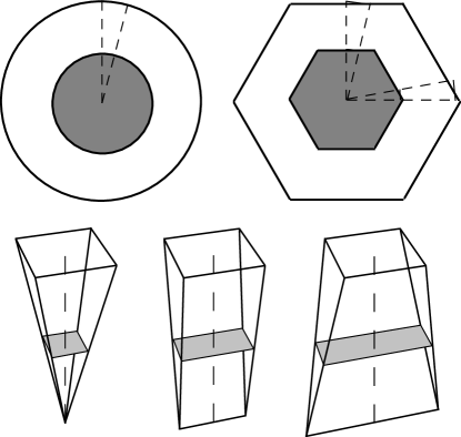
FIG. 3.: (Above) Hexagonal and round unit cells for the cylindrical phase, and (below) typical wedges for spherical, cylindrical, and bicontinuous phases; the dividing surface is shaded.

B Non-round unit cells (straight paths)

We can produce an upper bound for different structures by assembling small pieces of the cylindrical or spherical micelles to fill the appropriate unit cell. Each wedge has a parabolic monomer chemical potential given by eq 10. However, each wedge $\alpha$ has a slightly different shape and geometry, and thus has a distinct potential $\mu_{\alpha}$. Adjacent wedges are not in equilibrium with each other and will relax if allowed to do so. Hence the calculation yields an upper bound. To construct the unit cell of, e.g., hexagonal cylinders, we assume a hexagonal dividing surface scaled down by $\phi^{1/2}$ and assemble the unit cell from tiny pie-shaped wedges extending from the center of the hexagon to the cell boundary. We make an analogous construction for square arrays of cylinders, or for FCC and BCC packings of spheres.

We calculate the volume-averaged stretching free energy per molecule using eq 23. To calculate this in practice we use the following procedure. For cylindrical micelles we divide a cell of a given symmetry (say, hexagonal) into tiny wedges. Each wedge is adjusted slightly by making the segment of the wedge on the dividing surface normal to the bisector of the wedge, which is the path of the polymer. Such an adjustment introduces a negligible volume in the continuum limit of many small wedges. The surface area used for calculating the surface energy (eq 24) is, of course, the area of the segment in the original hexagonal dividing surface (before adjusting the wedge to account for straight paths).

FIG. 4.: Free energies of classical phases and the symmetric wedge, for straight-paths constructions (asymmetry factor $\varepsilon=1$). The shaded regions are bounded by the upper (BCC and HEX, respectively) and lower (spherical and cylindrical micelles, respectively) free energy bounds for the spherical and cylindrical topologies. The symmetric wedge has area function $a(\lambda)=2(\lambda-\lambda^{2})$, described in Sec. IV A.

For the classical phases (see Figure 4) the ratios of the upper and lower bounds for the free energies are independent of $\phi$, given by:

$$\begin{array}[]{lcccr}\displaystyle{f_{\mit hex}\over f_{\mit cyl}}&=&{\displaystyle\left({10\over 9}\right)^{1/3}}&\simeq&1.036\\ \vskip 10.0pt\cr\displaystyle{f_{\mit square}\over f_{\mit cyl}}&=&{\displaystyle\left({4\over 3}\right)^{1/3}}&\simeq&1.101\\ \vskip 10.0pt\cr\displaystyle{f_{\mit bcc}\over f_{\mit sph}}&=&{\displaystyle\left(95\over 384\right)^{1/3}\left({1\over 2}+\sqrt{3}\right)^{2/3}}&\simeq&1.072\\ \vskip 10.0pt\cr\displaystyle{f_{\mit fcc}\over f_{\mit sph}}&=&{\displaystyle\left({5\over 4}\right)^{1/3}}&\simeq&1.077.\end{array}$$ (29)

Evidently, the most favorable structures have the “roundest” unit cells. The hexagonal phase is favored over the square phase, and BCC is slightly favored over FCC.

C Non-round unit cells (kinked paths)

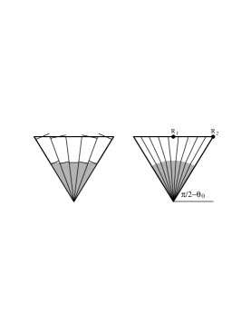
FIG. 5.: Hexagonal unit volume divided into wedges for straight-path (left) and kinked-path (right) ansatzes, for equal compositions $\phi$. Also indicated are adjustments necessary to calculate the free energy in each wedge for the straight-path ansatz.

Other upper bounds can be obtained by using different prescriptions for the $A\!-\!B$ surface. For example, one could choose a circular $A\!-\!B$ surface of radius $D(\phi)$ for the cylindrical phase. The inner ($A$) volume may be divided into wedges, and the outer ($B$) volume divided into wedges which each satisfy the volume constraint $\phi$ with a partner $A$ wedge [26]. For a right triangular wedge which subtends an angle $\theta_{0}$, points at angle $\theta$ on the $A\!-\!B$ surface map to points ${\rm\bf R}(\theta)$ on the boundary of the Wigner-Seitz cell,

$${\rm\bf R}(\theta)={\rm\bf R}_{1}+s\!\left(\theta\right)\left({\rm\bf R}_{2}-{\rm\bf R}_{1}\right)$$ (30)

where ${\rm\bf R}_{1}=\{0,1\}$, and ${\rm\bf R}_{2}=\{\tan\theta_{0},1\}$. The composition specifies the radius, according to

$$\phi\tan\theta_{0}=D^{2}(\phi)\theta_{0}.$$ (31)

The mapping which obeys the local composition constraint is

$$s(\theta)={\displaystyle{\theta\over\theta_{0}}-D(\phi){\sin\theta\over\tan\theta_{0}}\over 1-D(\phi)\cos\theta},$$ (32)

where $\theta_{0}=\pi/3$ and $\pi/4$ for hexagons and squares (see Figure 5), respectively.

Minimizing over the scale of the structure, eq 20 yields, after some calculation, the following free energy:

$${f\over f_{0}} = \left\{{2\phi\over 3}\left[\varepsilon^{-1}+{\varepsilon\phi^{2}\over(1-\phi)^{2}D^{4}(\phi)}\right.\right.\times$$ (34)

$$\left.\left.\int_{0}^{\theta_{0}}{d\theta\over\theta_{0}}|{\rm\bf R}-{\rm\bf r}|^{3}\left(3\left|{d{\rm\bf R}^{\prime}\over d\theta}\right|+\left|{d{\rm\bf r}^{\prime}\over d\theta}\right|\right)\right]\right\}^{1/3},$$

where

$${\rm\bf r}(\theta) = D(\phi){\sin\theta\choose\cos\theta}$$ (35)

$${\rm\bf r}^{\prime} = {\rm\bf r}\cdot\left[\mathchoice{{\hbox{\boldmath$\displaystyle\delta$}}}{{\hbox{\boldmath$\textstyle\delta$}}}{{\hbox{\boldmath$\scriptstyle\delta$}}}{{\hbox{\boldmath$\scriptscriptstyle\delta$}}}-{({\rm\bf R}-{\rm\bf r})({\rm\bf R}-{\rm\bf r})\over|{\rm\bf R}-{\rm\bf r}|^{2}}\right]$$ (36)

and similarly for $d{\rm\bf R}^{\prime}$. Remarkably, the upper bound for the kinked-path-hexagonal ansatz is typically less than $1\%$ above the lower bound of cylindrical micelles, and the transition is shifted to only a slightly smaller $A$ fraction $\phi$ (see Figure 6). Apparently the extra stretching energy to maintain a hexagonal $A\!-\!B$ interface with straight paths is relaxed considerably by allowing the inner block to adopt a more nearly circular dividing surface, which is preferred. Recent accurate numerical self-consistent field calculations of diblock melts have shown that in fact the $A\!-\!B$ interface is nearly circular, with a slight hexagonal modulation (angular modulation with 6-fold symmetry) of relative amplitude $0.03\%$ at $\chi N=60$ and $\phi=0.33$ [37].

FIG. 6.: Free energies for cylindrical topologies in various approximations (asymmetry factor ($\varepsilon=1$). Also shown is the free energy of the symmetric wedge. The inset shows an enlarged view of the crossing of the wedge and kinked-path-hexagonal free energies. The lamellar energy crosses the cylindrical micelle energy at $\phi=0.299$, the kinked-path-hexagonal energy at $\phi=0.293$, and the straight-path-hexagonal energy at $\phi=0.255$.

IV Geometry of bicontinuous phases

A Generic saddle surfaces

Before addressing particular symmetries (P, D, or G) of bicontinuous phases, we discuss the closest analogue to a round unit cell. We would like to produce a simple estimate of the free energy, analogous to the cylindrical and spherical micelle calculation, which captures the physics of bicontinuous topologies. We thus represent a generic bicontinuous phase as a wedge, shown in Figure 7: an infinitesimal patch of “saddle” surface, with edges given by the normals, terminating in a small line segment lying along the bond-lattice. We envision the surface as a minimal surface, which has zero mean curvature.[38]

The stretching free energy per molecule of the symmetric wedge can be calculated as before, given the relative area as a function of relative height along the center normal (Table I): $a(\lambda)\!=\!\lambda(2-\lambda)$, where $\lambda\!=\!z/R$, $z\!=\!0$ is the thin end of the wedge and $z\!=\!R$ is the patch of minimal surface. As before, the dividing surface location $z_{d}$ is determined by eq 5. The resulting free energy is given by applying eqs 5-7, and is shown with the various cylindrical bounds in Figure 6. This estimate misses by a few tenths of one percent the intersection of the lamellar phase and the kinked-path upper bound bound for the hexagonal phase, and is stable with respect to the straight-path upper bound.

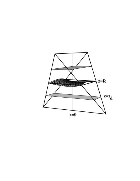
FIG. 7.: Symmetric saddle chip ($p\!=\!2$ in Eq. 3). The $A\!-\!B$ dividing surface at $z\!=\!z_{d}$ is shaded. $A$ material fills the top and bottom of the wedge, and $B$ material fills the volumes near the (minimal) partitioning surface.

Clearly the simple wedge construction captures some important physics. The structures formed by copolymers at different volume fractions $\phi$ arise from competition between interfacial and stretching free energies. The different structures present different functions $a(\lambda)$, which determine both the dividing surface area and the stretching energy as a function of volume fraction. The phases occur in the order they do because the progression of functions $a(\lambda)$ from quadratic $\lambda^{2}$ (spheres) to linear $\lambda$ (cylinders) to $\lambda(2-\lambda)$ (bicontinuous) to constant (lamellae) gives progressively less volume to the “outer” chain to avoid stretching, but uses progressively less area to separate the two species at higher volume fractions of the minority species.

FIG. 8.: Free energies for saddle wedges of various shape factors $p=1.5,1.9,2.0,2.1$. Also shown is the free energy of the kinked-path hexagonal phase.

However, we cannot argue as before that our simple estimate for the bicontinuous phase is a lower bound for actual bicontinuous phases, because there is no way to pack together copies of one infinitesimal wedge to produce a “micelle” that 1) fills some region of space, and 2) is bounded by some surface(s), the volume outside of which could be filled by homopolymer. Neither can we argue that this estimate is an upper bound, because we certainly cannot pack a unit cell of the region bounded by the D or G surfaces with identical copies of one infinitesimal wedge.

Bicontinuous phases are assembled from different wedges $\alpha$, with different shape factors $p_{\alpha}$ in Table I. The shape factor roughly gauges the splay or Gaussian curvature of the surface at the top of the wedge, with $p=1$ (cylinders) corresponding to zero Gaussian curvature, $p<1$ to positive Gaussian curvature, and $p>1$ to negative Gaussian curvature. [The Gaussian curvature is the product of the two radii of curvature of a surface]. The distribution of wedges must be chosen to pack the desired structure. While the symmetric wedge has $p=2$, this is not an optimum shape. In fact, the optimum wedge shape depends on composition, as can be seen in Figure 8. It is evident that there are shape factors $p$ which have lower free energy than the straight- and kinked-path hexagonal upper bounds (Figure 9), so it is not unreasonable to hope that a judicious packing configuration can be a stable thermodynamic phase.

The effect of the shape factor $p$ on the topology of the phase diagram emerges upon examining conformationally asymmetric ($\varepsilon\neq 1$) copolymers. Following Ref. [25], we explore the effect of conformational asymmetry on the stability of bicontinuous phases by multiplying the wedge free energy by an additional arbitrary small prefactor $(0.99)$ which enhances stability. [We will see below that for $\varepsilon=1$ the bicontinuous phases that we can calculate (G, D, P) are of order $0.3-2.2\%$ higher than the cylinder-lamellar crossing, depending on which upper bound one compares.] Figure 10 shows ‘phase diagrams’ as a function of conformational asymmetry $\varepsilon$.

Recall that for $\varepsilon>1$ the $B$-block is more flexible, while the $A$-block is stiffer and better able to stretch. For the symmetric wedge $(p=2)$ conformational asymmetry reduces the stability of the stiff-minority wedge phase $(\phi<1/2)$ and enhances the stability of the flexible-minority wedge phase ($\phi>1/2$), and shifts all transitions to greater $\phi$. For $p>2.0$ the wedge phases lose stability, as could be guessed from Figure 9. For $p<2.0$, for which the wedge is more cylindrical-like ($p=1$ coresponds to cylinders), conformational asymmetry enhances the stiff-minority wedge phase relative to both the lamellar and cylindrical phases, and decreases the stability of the flexible-minority wedge phase. We emphasize that these are not phase diagrams, for a true phase is a mixture of wedges with different shape factors which fill space.

FIG. 9.: Free energy relative to that of the kinked-path hexagonal phase, as a function of saddle wedge shape factor $p$, for compositions $\phi=0.28,0.31,0.35$.

FIG. 10.: Phase diagrams for the round unit cell approximation, including the saddle wedge for shape factors $p=1.8,1.9,2.0,2.1$, as a function of composition $\phi$ and conformational asymmetry $\varepsilon$. The free energy of the wedge has been multiplied by an additional prefactor $(0.99)$ to explore the effect of conformational asymmetry on the stability of bicontinuous phases.

B Conformational Asymmetry

Experimentally, the G phase has been observed between the lamellar and cylindrical phases in several strongly-segregated copolymer systems, for $\phi$ around 0.3 (and, symmetrically, around 0.7). Some groups have argued for phase stability of bicontinuous phases in terms of bending rigidities,[39, 40]. However, there is fundamentally no bending energy in the problem; descriptions in terms of bending energies only arise from a proper accounting of stretching free energy in curved geometries. Our approach is to choose a geometry as an ansatz and compute the corresponding interfacial and stretching free energies in a manner consistent with calculations for cylindrical, spherical, and lamellar phases. The structure, revealed by scattering and electron microscopy,[11, 13] studies, can be described as follows,[38, 41].

Consider first the D geometry, which is easier to visualize. A skeleton formed of the bonds of a diamond lattice is shown in Figure 11. Two such lattices interpenetrate, analogous to the interpenetration of two simple cubic lattices in a BCC structure. Now imagine swelling the bonds in these lattices into tubes of a finite diameter. The walls of these tubes are a rough approximation of the experimentally observed “dividing surface” separating the regions containing the two blocks. The volume contained within the tubes corresponds to the region inhabited by the low volume-fraction monomer.

To model the D geometry, we use a self-dual minimal surface, called the Schwartz D (diamond) surface, which partitions space into two identical interpenetrating regions, each of which contains and is topologically equivalent to a diamond bond-lattice [8, 10, 41]. Within each of these regions is a dividing surface, which surrounds a copy of the bond-lattice. The copolymer chains then have conformations with one (A) species stretching towards the bond-lattice, the junction between blocks residing on the dividing surface, and the other (B) species stretching towards the minimal surface. In the G phase the diamond lattice is replaced by a three-fold coordinated lattice, and the surface is replaced by the gyroid minimal surface discovered by Schoen in 1970 [14], in which the two interpenetrating G volumes are chiral enantiomers of one another. For the P phase the bond lattice is six-fold coordinated (Figure 11) and the candidate partitioning surface is the Schwartz P minimal surface.

There is no compelling reason to choose a minimal surface for the partitioning surface. However, minimal surfaces solve the variational problem of minimizing surface area with zero pressure across the interface. If the diblock phase is in fact partitioned into two equivalent connected regions, then by symmetry there can be no net pressure exerted across the dividing surface that separates the two equivalent disjoint connected regions. So a minimal surface is reasonable, but by no means certain, since there is no obvious area energy to minimize.

FIG. 11.: Skeleton bond lattices for, from top to bottom, the P, D, and G surfaces.

The P, D, and G surfaces may be conveniently calculated using the Weierstrass representation.[38] Here, the three-dimensional points ${\rm\bf r}$ of the two-dimensional surface are parametrized by the complex number $\omega=\omega_{1}+i\omega_{2}$. The G, P, and D surfaces are triply-periodic minimal surfaces with space groups $Ia\bar{3}d,Im\bar{3}m,$ and $Pn\bar{3}m$, respectively.[14] To generate the full surface it is enough to calculate a single patch, to which all the symmetry operations of the space group may be applied to generate the full structure. A generic surface has two radii of curvature which are generally non-zero and different. Points where the surface is flat are singular points, since both radii of curvature are zero and a direction of the surface cannot be determined. These flat points define the corners of the fundamental patch.

The Weierstrass representation is:

$${\rm\bf r}=\hbox{Re}\int_{{\cal V}}{{\rm\bf v}(\omega)\,e^{i\theta}\over(\omega^{8}-14\omega^{4}+1)^{1/2}}d^{2}\!\omega,$$ (37)

where

$${\rm\bf v}(\omega)=\left\{1-\omega^{2},i\left(1+\omega^{2}\right),2\omega\right\},$$ (38)

and ${\cal V}$ is the domain of integration shown in Figure 12. The points on the corners correspond to the flat points, and it is evident that the integrand above (excluding the measure) is singular at these points. The angle $\theta$ determines the surface:

$$\theta=\left\{\begin{array}[]{c@{\quad}l}0&\hbox{D\quad($Pn\bar{3}m$)}\\ 90^{\circ}&\hbox{P\quad($Im\bar{3}m$)}\\ 38.015^{\circ}&\hbox{G\quad($Ia\bar{3}d$)}\end{array}\right.$$ (39)

FIG. 12.: The thick line bounds the domain of integration ${\cal V}$ for the Weierstrass representation. The arcs are from circles of radius $\sqrt{2}$ centered at the points $(\pm 1,\pm 1)/\sqrt{2}$.

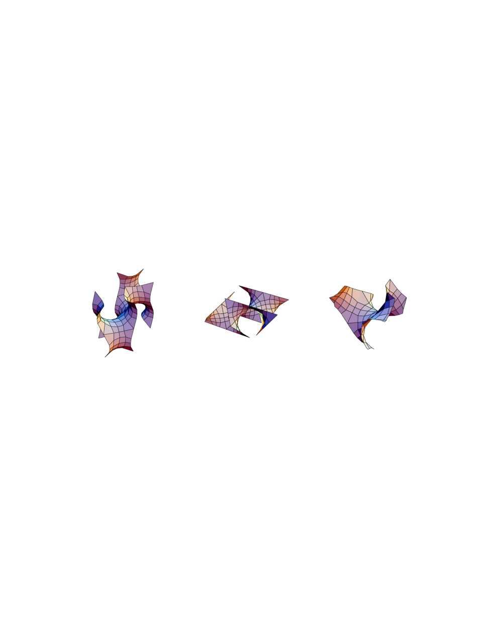
FIG. 13.: Top: fundamental patches of, from left to right, the P, D, and G surfaces. Below: larger portions of the surfaces.

For other angles the surface intersects itself. This does not, of course, exhaust the class of triply periodic minimal surfaces either mathematically,[14, 41, 42] or physically [43]. We have chosen the D, P, and G surfaces because they are the most common observed surfactant bicontinuous surfaces, and have been claimed experimentally in block copolymers. Sections of these surfaces are shown in Figure 13 For fairly accurate calculations (yielding energies lower than those for the true surface by of order a few tenths of a percent) the D surface may be approximated by a simple hyperbolic surface, $z=xy$. This suggests that the minimal D surface may not the optimal partitioning surface. However, we have varied the shape of the partitioning surface around the D surface, and found free energy variations of only a few tenths of a percent. Because of this, we have not optimized the free energy with respect to adjustments in the partitioning surfaces.

To produce an upper bound on the free energy of the bicontinuous phases we follow a procedure analogous to that used for the classical cylindrical and spherical topologies. Namely, we divide a unit cell of these structures into a large number of wedges (shown in Figure 14), similar to Figure 1, but of varying radii and Gaussian curvature, and average the free energy per molecule using eq 23-25. Each structure has a different unit cell (a big wedge) from which the entire structure may be generated by applying the symmetry operations of the particular space group. Figure 15 shows the fundamental cell for the G structure.

This procedure is straightforward. First we calculate the minimal surface, and then adopt a convenient mapping from the points on this surface to the skeleton. Essentially, we construct an interpolation between those high-symmetry points on the minimal surface with normals that project onto the underlying bond-lattice. For the $D$ and $G$ phases, we optimize the mapping from the partitioning surface to the line segments of the bond lattice to minimize the free energy. We perform this by a conjugate gradient algorithm that distorts the two dimensional mesh of points on the surface, and gains of order $1\%$ in energy.

FIG. 14.: Fundamental wedges used for constructing the D or P (left) and G (right) structures. We have shown quite general wedges, before they undergo slight adjustments to ensure that ${\bf\hat{n}}$ is normal to the bond segment ${\rm\bf z}_{1}\!-\!{\rm\bf z}_{2}$ and the surface element ${\rm\bf a}{\rm\bf b}{\rm\bf c}{\rm\bf d}$.

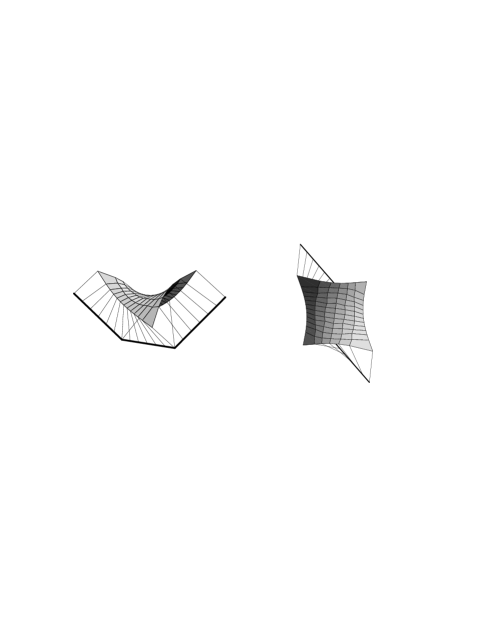
FIG. 15.: Side and top views of basic unit for G structure, showing the initial division into wedges.

Thus, each small patch on the minimal surface is connected by straight lines to a small line segment on the skeleton, and a set of wedges results. Each wedge is adjusted slightly by making both the top patch and the bottom segment orthogonal to the line segment connecting the center of the patch to the skeleton. This is analogous to making the outer surface of the wedge in the upper bound for the hexagon phase orthogonal to the line segment connecting the center of the outer surface of the wedge to the center of the hexagon. Such adjustments are negligible in the limit of infinitesimal wedges. As before, the area of the $A\!-\!B$ interface is the true area, rather than the (smaller) area that results from adjusting the wedge to assure a chain path normal to the $A\!-\!B$ interface.

In this way, the unit cell of the region bounded by a minimal surface is decomposed into many small wedges, each with a known (and different) radius $R$, shape factor $p$, and volume. The location of the dividing surface within each wedge is fixed by eq 22, and the free energy calculated with eqs 23-25. We have checked the algorithm and the dependence on the fineness of the mesh by using it to successfully compute the free energies of the hexagonal phase.

V Results

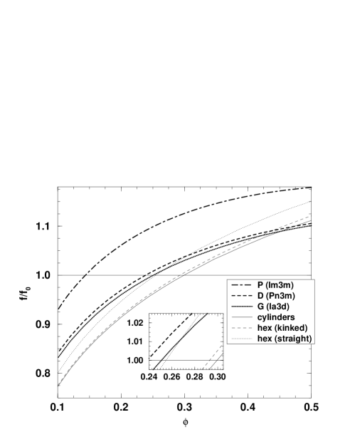
FIG. 16.: Free energies for bicontinuous phases (upper bounds) compared to upper and lower (cylinders) bounds of the hexagonal phase. The inset enlarges the crossing of the G and straight-path-hexagon upper bounds. Asymmetry parameter $\varepsilon=1.0$.

Figure 16 shows the free energy curves as a function of $\phi$ for conformationally symmetric copolymers ($\varepsilon=1$). The upper bound for the $Im\bar{3}m$ phase (P) lies $4-5\%$ above that for the $Pn\bar{3}m$ phase (D), which in turn is less than a percent ($\simeq 0.7\%$ at $\phi=0.3$) above the $Ia\bar{3}d$ (G) phase. Consistent with experiments and self-consistent field theory, we do not find a stable G phase. At the lamellar–kinked-path-hexagons free energy crossing ($\phi\simeq 0.293$) the free energy of the $G$ phase is of order $2.2\%$ larger, while at the lamellar–straight-path-hexagons free energy crossing ($\phi\simeq 0.255$) the free energy of the $G$ phase is only a few tenths of a percent ($\simeq 0.28\%$) greater. This, we have argued, may be the fairer comparison, since both calculations use straight paths. Unfortunately, we do not know how to perform a kinked-paths estimate for the bicontinuous phases.

Note, however, that we do not expect to gain as much energy from a kinked-path calculation for the bicontinuous phases as for the cylindrical topologies. Consider the hexagonal calculation. The boundaries of the Wigner-Seitz cell, and hence the $A\!-\!B$ dividing surface, have sharp corners into which the chains must stretch. Presumably a large part of the gain in the kinked-path calculation comes from relieving the strain associated with this stretch, and relaxing the inner block to its preferred circular structure. Bicontinuous phases, on the other hand, have smooth “Wigner-Seitz boundaries” (i.e. the minimal surface), and expensive stretching occurs mainly at the junctions of the skeleton lattice. Hence, the anomalous stretching that may be relieved by a kinked-path calculation occurs along points in the structure, rather than along lines. So we expect that our straight-path estimate is not likely to differ greatly from a kinked-path estimate, and that the free energy of the G phase remains well above that of the kinked-path hexagons. The stretching of the chains at the junctions presumably contributes to the relative stability of the $P$, $D$, and $G$ structures, which have 6-, 4-, and 3-fold coordinated bond lattices. The more highly-coordinated lattices require more chain stretching to accommodate the space, which suggests that $P$, $D$, and $G$ occur in increasing order of stability. This picture is corroborated by recent work of Matsen and Bates [44], who quantitatively examined the packing frustration in the G, D, and HPL phases.

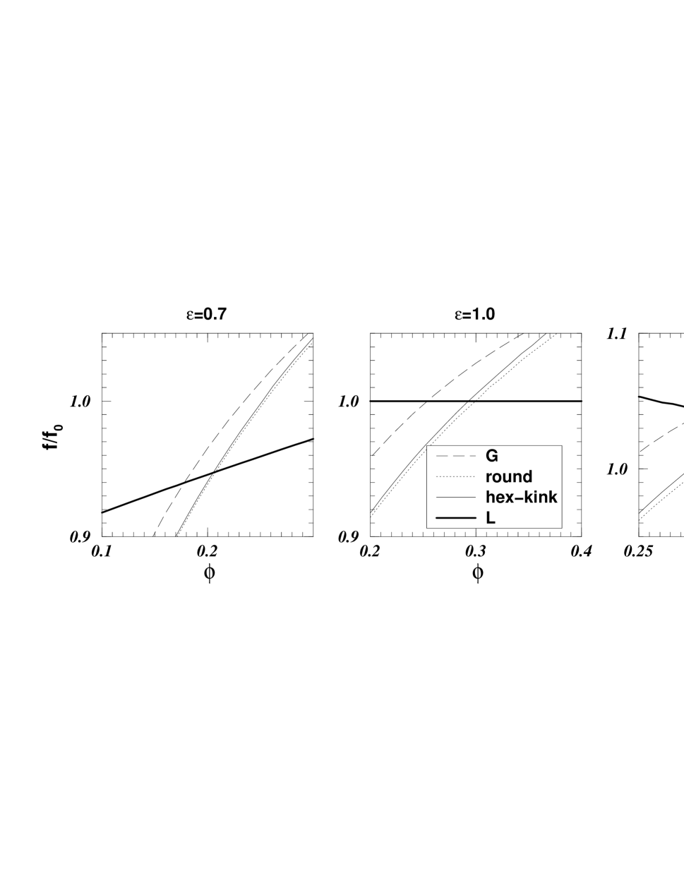
FIG. 17.: Free energy crossings for gyroid, hexagonal (kinked paths) and lamellar phases for asymmetry parameter values $\varepsilon=0.7,1.0,$ and $1.3$. For $\varepsilon>1$ the species ($B$) with composition $1\!-\!\phi$ is more flexible and/or has more arms than the other ($A$) species, and the $A$ species has an enhanced tendency to stretch.

Our results apply to the strong-segregation limit, which is attained in the limit of large $\chi$. Because the phase boundaries shift away from $\phi=0.5$ as $\chi$ increases from weak segregation [3], we expect our phase boundaries to be further from $\phi=0.5$ than experimental values, which is indeed the case.

Figure 17 shows free energy crossings for various values of the conformational asymmetry parameter $\varepsilon$. Relative to a conformationally symmetric melt, conformational asymmetry stabilizes phases with a stiff minority species and destabilizes phases with a stiff majority species, moving boundaries to larger $\phi(A)$ for $\varepsilon>1$. Recall that for $\varepsilon<1$ the inner $A$-block is more flexible, while the $B$-block is stiffer and better able to stretch. We find that $\varepsilon<1$ reduces the relative stability of the G phase, while the stability is enhanced for $\varepsilon>1$, and becomes stable for rather large asymmetries $\varepsilon\gtrsim 9.0$ (Figure 18).

FIG. 18.: Free energy of G phase relative to that of the kinked-path upper bound estimate of the lamellar-hexagonal phase boundary, as a function of conformational asymmetry $\varepsilon$. The vertical line marks the conformationally symmetric copolymer, and the horizontal line is for reference.

Previous calculations of phase diagrams of conformationally-asymmetric diblocks have been done in the weak segregation regime,[45, 46] and, for the generic symmetric wedge as a model bicontinuous structure, in the strong segregation regime.[25] Matsen and Bates [46] found, as we do, that conformational asymmetry stabilizes the G phase with a stiff minority phase, widening the composition window and moving the lamellar-G and G-cylinder boundaries to higher stiff compositions; and destabilizes the G phase with a stiff majority phase, both narrowing the composition window and shifting it to a higher stiff fraction. Their calculations are limited to $\chi N\lesssim 30$, and it is inconclusive whether the $\chi N\rightarrow\infty$ limit of this calculation yields a stable G phase. The same qualitative behavior was found for the generic symmetric wedge in the strong segregation regime.[25]

Table II summarizes asymmetry parameters from recently collected data [47, 48]. While none of these diblocks have the large conformational asymmetry required to test our prediction of a stable phase in strong segregation, $A_{n}-B_{m}$ starblock copolymers have asymmetry factors larger, by a factor of $n/m$, than those due to intrinsic chain stiffness effects alone. For example a $\hbox{PE}_{6}$–$\hbox{PEE}_{1}$ starpolymer has an asymmetry factor $\varepsilon\simeq 6\times 1.58=9.48$.

We have attempted to calculate energies for the HPL [28, 29] phase, which is now accepted as a metastable phase [31]. The minimal crystal phases D, P, and G have obvious candidate minimal surfaces to act as an intermaterial dividing surface towards which the majority-phase ends stretch; and the minority-phase ends stretch towards the skeletal bond lattice. On the other hand, the majority-phase ends in the HPL phase stretch towards a combination of lines (in the hexagonally-arranged perforating tubes) and surfaces (within the majority-phase layer). Similarly, it is not obvious how to partition the minority-phase ends between lines and surfaces. The result is a non-analytic mapping which is difficult to minimize over. Our attempts have thus far yielded quite high energies, of order that of the $P$ phase.

VI Summary

We have outlined a general method for computing the free energy of block copolymer phases in the strong segregation regime. The procedure consists of the following steps:

1. Choose a candidate geometry and an associated partitioning surface that divides space into disjoint interpenetrating regions (the majority blocks from the two regions stretch towards this surface).

2. Divide the enclosed volume into infinitesimal wedges, defined by straight paths connecting the partitioning surface to a skeleton of bonds (the minority blocks stretch towards this bond skeleton).

3. The A-B interface in each wedge is located such that the fraction of wedge volume filled by A blocks is locally equal to $\phi$. The interfacial contribution to the free energy is the area of the A-B interface times the A-B surface tension.

4. Compute the stretching free energy per chain for each wedge within the approximation of straight paths. Calculations for straight paths involve slight adjustments to the wedges whose contributions vanish in the limit of small wedges.

5. Optimize the free energy per chain with respect to the overall scale of the mesophase (e.g., the dimension of the unit cell).

6. Optimize the mapping from the partitioning surface to the bond skeleton to minimize the overall free energy.

In certain structures (e.g. HPL) the majority phase ends lie on both lines and surfaces, in which case the procedure above must be suitably generalized. We have also shown how to calculate the free energy for geometries where the shape of the $A\!-\!B$ interface is specified, for phases of cylindrical topology. This requires polymer chain paths which are kinked at the $A\!-\!B$ interface.

The infinitesimal wedges are described by the relative area function $a(z/R)$ (eq 2) which is parametrized by a single scalar $p$ (eq 3 and Table I) that roughly gauges the local Gaussian curvature of the partitioning surface. For the classical phases all wedges are identical, while bicontinuous phases have different distributions of shape factors $p$. For symmetric stars we find a metastable bicontinuous (gyroid, or G) phase which is most stable near the lamellae-hexagonal cylinder transition. For sufficiently asymmetric copolymers ($\varepsilon\gtrsim 9.0$) we predict a stable G phase.

REFERENCES

- [1] Bates, F. S. Science 1991, 251, 898.
- [2] Bates, F. S.; Fredrickson, G. H. Ann. Rev. Phys. Chem. 1990, 41, 525.
- [3] Leibler, L. Macromolecules 1980, 13, 1602.
- [4] In a weakly segregated mesophase, very long polymer chains are in fact more strongly stretched than Gaussian chains [Almdal, K.; Rosedale, J. H.; Bates, F. S.; Wignall, G. D.; and Fredrickson, G. H. Phys. Rev. Lett. 1990, 65, 1112], which has been explained in terms of concentration fluctuations [Barrat, J.-L.; and Fredrickson, G. H J. Chem. Phys. 1991, 95, 1281].
- [5] Helfand, E.; Wasserman, Z. R. In Developments in Block Copolymers; Goodman, I. Ed.; Applied Science: New York, 1982; Vol. 1.
- [6] Semenov, A. N. JETP 1985, 88, 1242.
- [7] Olmsted, P. D.; Milner, S. T. Phys. Rev. Lett. 1994, 72, 936; ibid, 1995, 74, 829.
- [8] Thomas, E. L.; Alward, D. B.; Kinning, D. J.; Martin, D. C.; Handlin, D. L.; Fetters, L. J. Macromolecules 1986, 19, 2197.
- [9] Hasegawa, H.; Tanaka, H.; Yamasaki, K.; Hashimoto, T. Macromolecules 1987, 20, 1641.
- [10] Anderson, D. M.; Thomas, E. L. Macromolecules 1988, 21, 3221.
- [11] Hajduk, D.A.; Harper, P.E.; Gruner, S.M.; Honeker, C.C.; Kim, G.; Thomas, E.L.; Fetters, L.J. Macromolecules 1994, 27, 4063; Hajduk, D.A.; Gruner, S.M.; Rangarajan, P.; Register, R.A.; Fetters, L.J.; Honeker, C.; Albalak, R.J.; Thomas, E.L. Macromolecules 1994, 27, 490; Hajduk, D.A.; Harper, P.E.; Gruner, S.M.; Honeker, C.C.; Thomas, E.L.; Fetters, L.J. Macromolecules 1995, 28, 2570.
- [12] Forster, S.; Khandpur, A.K.; Zhao, J.; Bates, F.S.; Hamley, I.W.; Ryan, A.J.; and Bras, W. Phys. Rev. Lett. 1994, 27, 6922.
- [13] Schulz, M.F.; Khandpur, A.K.; Bates, F.S.; Almdal, K.; Mortensen, K.; Hajduk, D.A.; Gruner, S.M. Macromolecules 1996, 29, 2857.
- [14] Schoen, A. H. NASA Tech. Note 1970, TN D-5541, 1.
- [15] Mayes, A.M.; de la Cruz, M.O. J. Chem. Phys. 1991, 95, 4670.
- [16] Jones, J.L.; de la Cruz, M.O. J. Chem. Phys. 1994, 100, 5272.
- [17] Hamley, I.W.; Bates, F.S. J. Chem. Phys. 1994, 100, 6813.
- [18] Matsen, M.W.; Schick, M. Phys. Rev. Lett. 1994, 72, 2660; Macromolecules 1994, 27, 7157.
- [19] Matsen, M.W.; Bates, F.S. Macromolecules 1996, 29, 1091.
- [20] Milner, S. T.; Olmsted, P. D. J. Phys. II (France) 1997, 7, 249.
- [21] Podneks, V. E.; Hamley, I. W. JETP Lett. 1996, 64, 617.
- [22] Likhtman, A.E.; Semenov, A.N. Macromolecules 1994, 27, 3103.
- [23] Milner, S. T.; Witten, T. A.; Cates, M. E. Europhys. Lett. 1988, 5, 413; Macromolecules 1988, 21, 2610.
- [24] Milner, S.T. J. Poly. Sci., Part B 1994, 32, 2743.
- [25] Milner, S.T. Macromolecules 1994, 27, 2333.
- [26] Xi, H.W.; Milner, S.T. Macromolecules 1996, 29, 2404.
- [27] Matsen, M.W.; Bates, F.S. Macromolecules 1995, 28, 8884.
- [28] Hamley, I. W.; Koppi, K. A.; Rosedale, J. H.; Bates, F. S.; Almdal, K.; Mortensen, K. Macromolecules 1993, 26, 5959.
- [29] Disko, M. M.; Liang, K. S.; Behal, S. K.; Roe, R. J.; Jeon, K. J. Macromolecules 1993, 26, 2983.
- [30] Fredrickson, G. H. Macromolecules 1991, 24, 3456.
- [31] Hajduk, D. A.; Takenouchi, H.;Hillmyer, M.; and Bates, F. S., to be published.
- [32] The composition variable is defined in Ref. [25] as the volume fraction of the phase. Similarly, Ref. [25] defines with and reversed with respect to the present article, so equations such as eqs 26-28 are identical in the two works (compare eqs 9-11 of Ref. [25]). Eq 8 of Ref. [25] has a misprint, and should have a factor of to match eq 19 in Section II above.
- [33] Helfand, E.; Tagami, Y. J. Polym. Sci 1971, B9, 741.
- [34] Ball, R. C.; Marko, J. F.; Milner, S. T.; Witten, T. A. Macromolecules 1991, 24, 693.
- [35] Bates, F.S.; Fredrickson, G.H. Macromolecules 1994, 27, 1065.
- [36] Almdal, K.; Rosedale, J.H.; Bates, F.S. Macromolecules 1990, 23, 4336.
- [37] Matsen, M. W.; Bates, F. S. J. Chem. Phys. 1997, 106, 2436.
- [38] Nitsche, J. C. C. Lectures on Minimal Surfaces; Cambridge University Press: Cambridge, 1989.
- [39] Ajdari, A.; Leibler, L. Macromolecules 1991, 24, 6803.
- [40] Wang, Z.-G.; Safran, S. A. J. Phys (France) 1990, 51, 185.
- [41] Anderson, D. M.; Davis, H. T.; Scriven, L. E.; Nitsche, J. C. C. Adv. Chem. Phys. 1990, 77, 337.
- [42] Góźdź, W. J.; Hołyst, R. Phys. Rev. Lett. 1996, 76, 2726; Phys. Rev. 1996, E54, 5012.
- [43] Luzzati, V.; de la Croix, H.; Gulik, A. J. Phys. II (France) 1996, 6, 405.
- [44] Matsen, M. W.; Bates, F. S. Macromolecules 1996, 29, 7641.
- [45] Vavasour, J. D.; Whitmore, M. D. Macromolecules 1993, 26, 7070.
- [46] Matsen, M. W.; Bates, F. S. J. Poly. Sci: Poly. Phys. 1997, 35, 945.
- [47] Fetters, L. J.; Lohse, D. J.; Richter, D.; Witten, T. A.; Zirkel, A. Macromolecules 1994, 27, 4639.
- [48] Bates, F. S.; Schulz, M. F.;Khandpur, A. K.; Förster, S.; Rosedale, J. H.; Almdal, K.; and Mortensen, K. Faraday Discuss. 1994, 98, 7.