Critical properties of the topological Ginzburg-Landau model

Abstract

We consider a Ginzburg-Landau model for superconductivity with a Chern-Simons term added. The flow diagram contains two charged fixed points corresponding to the tricritical and infrared stable fixed points. The topological coupling controls the fixed point structure and eventually the region of first order transitions disappears. We compute the critical exponents as a function of the topological coupling. We obtain that the value of the $\nu$ exponent does not vary very much from the $XY$ value, $\nu_{XY}=0.67$. This shows that the Chern-Simons term does not affect considerably the $XY$ scaling of superconductors. We discuss briefly the possible phenomenological applications of this model.

Pacs numbers: 74.20De, 11.10Hi.

I Introduction

The Ginzburg-Landau model (GL) has been introduced almost half a century ago [1] as a phenomenological model for superfluidity and superconductivity. In its one component order parameter version it has been used with remarkable success as a statistical mechanics model for the critical phenomena of systems lying in the same universality class as the Ising model [2]. In its $N$ component version coupled to Abelian gauge fields it has been used as a model for superconductivity and liquid crystals [3]. However, in this last situation the $\epsilon$-expansion, which works very well in the non-gauged version, seems to be insufficient to describe unambiguously the critical properties of the model [4, 5]. Only in the large $N$ limit the $\epsilon$-expansion gives consistent results [4]. The trouble is the absence of a second order (infrared stable) fixed point in the flow diagram. This result is physically correct only in the extreme type I regime $u/e^{2}<<1$ (here $u$ is the quartic scalar self-coupling and $e$ is the charge), where we expect a weak first order phase transition. This regime is also well described by the fluctuation corrected mean field analysis of Halperin et al. [4]. The weak first order transition has been probed experimentally in certain classes of liquid crystals, where essentially the same GL model holds [6]. For the extreme type II region ($u/e^{2}>>1$), a second order fixed point is expected. Indeed, this result follows from numerical studies performed in a lattice dual GL model [7]. Therefore, the prediction of a first order transition even in the type II regime seems to be an artifact of the $\epsilon$-expansion. More recent works support also this point of view [8, 10, 11, 9, 15]. Also, it has been shown that the renormalization group (RG) in a fixed dimension approach is more appropriate [8, 10, 11]. The flow diagram in the $u-e^{2}$ plane exhibits in general four fixed points: Gaussian and superfluid (or XY), both uncharged, and the tricritical and superconducting which are charged fixed points. The Gaussian fixed point is trivial and describes the mean field critical behavior of a $O(2)$ model (we shall work with $N=2$). The superfluid fixed point describes the $\lambda$-transition in $He^{4}$ and lies in the same class of universality as the XY model. The tricritical fixed point is over a line, called tricritical line, which separates the regions of first and second order phase transition. This fixed point is attractive along the tricritical line but repulsive in the direction nearly parallel to the $u$-axis. Finally, the superconducting fixed point is a charged infrared stable fixed point and describes a second order superconducting phase transition. Bergerhoff et al. [10] obtained this flow diagram using Wilson’s RG [12] in a non-perturbative version called exact renormalization group [13]. They used the background field formalism to control gauge invariance which is in principle violated due to the presence of the cutoff (further discussions on this subtle point in Wilson’s RG can be found in refs.[14]). This flow diagram has been also obtained by Herbut and Tesanovic [11] using a simpler method. They performed a 1-loop calculation in a fixed dimension approach.

Recently a flow diagram with qualitatively the same structure has been also obtained for a GL model with a topological Chern-Simons (CS) term by Malbouisson et al. [16]. Their analysis was performed using Wilson’s RG in perturbative form, which is not manifestly gauge invariant due to the cutoffed integrals. Due to the presence of a CS term, an intrinsically three dimensional object, their calculations were performed in $d=3$ and $N=2$, resulting therefore in an uncontrolled approximation since there is no small parameter as $\epsilon$ or $1/N$. The same type of model has been considered earlier by Kleinert and Schakel [17] using a different scaling. They performed a 1-loop calculation of critical exponents. However, their scaling did not allows for a consistent zero CS mass limit since Feynman graphs were evaluated at zero external momenta. The reason comes from the graph shown in Fig.1. When evaluated at zero external momenta this graph gives zero due to the structure of the CS gauge field propagator. On the other hand, in the same scaling this graph is infrared divergent if no CS mass is included in the action. Thus, it is not legitimate to perform the zero CS mass limit in the scaling considered in [17] as observed by the authors themselves. There are many other RG studies of bosonic CS models in the literature but the $F^{2}$ term is almost always absent [18]. The presence of such a term is crucial in order to obtain the flow diagram of ref. [16]. Moreover, it is desirable to recover the usual GL model in the limit of zero CS mass.

In this paper we consider further the topological model of refs. [16, 17], performing the calculation at the critical point [2]. We consider two different approximations. In a first step (section II) we perform a 1-loop calculation of the RG functions assuming that the same scale holds for both the order parameter and the gauge field. In this context we find the following main features: (1) For the CS coupling smaller than a certain critical value there are no charged fixed points; (2) There exists a interval of CS couplings such that two charged fixed points are found, corresponding respectively to the tricritical and second order (infrared stable) fixed points. In this interval it is possible to find respectable values for the $\nu$ exponent but not for the $\eta$ exponent, eventually violating the scaling relations; (3) For larger CS coupling, outside the interval mentioned in (2), the region of first order behavior is lost since the tricritical fixed point assumes an unphysical value. The second step (section III) consists in improving upon the 1-loop result of section II by distinguishing the scales of the order parameter and the gauge field. In this approximation we follow an idea of Herbut and Tesanovic in order to relate both scales and obtain in this way the RG flow. In this case we have the tricritical and second order fixed points even in the limit of zero CS coupling, consistent with the fixed point structure of the conventional GL model. However, once again the tricritical fixed point becomes unphysical for the CS coupling larger than a certain critical value. In this case we obtain that all the critical exponents have respectable physical values. Moreover, the $\nu$ exponent as a function of the topological coupling does not deviate very much from $XY$ scaling. Finally, in section IV we discuss our results and the possible applications.

II Model and RG results

Our starting point is the following action:

$$S = \int d^{3}x\left[|(\nabla-ie_{0}\vec{A}_{0})\psi_{0}|^{2}+r_{0}|\psi_{0}|^{2}+\frac{u_{0}}{2}|\psi_{0}|^{4}\right.$$ (1)

$$+ \left.\frac{1}{8\pi\mu_{0}}(\nabla\times\vec{A}_{0})^{2}+i\frac{\theta_{0}}{2}\vec{A}_{0}\cdot(\nabla\times\vec{A}_{0})\right]+S_{gf},$$ (2)

where the subindex $0$ denotes bare quantities. The above action is a standard GL model with a CS term added. $S_{gf}$ is the gauge fixing term which is given by

$$S_{gf}=\int d^{3}x\frac{1}{2\alpha_{0}}(\nabla\cdot\vec{A}_{0})^{2},$$ (3)

with $\alpha_{0}$ being the bare gauge fixing parameter. The bare propagator for the gauge field is given by

$$D_{ij}(k) = \frac{4\pi\mu_{0}}{k^{2}+g^{2}_{0}}\left[\delta_{ij}-\frac{k_{i}k_{j}}{k^{2}}-g_{0}\frac{\epsilon_{ijk}k_{k}}{k^{2}}\right.$$ (4)

$$+ \left.\frac{\alpha_{0}}{4\pi\mu_{0}}\left(1+\frac{g_{0}^{2}}{k^{2}}\right)\frac{k_{i}k_{j}}{k^{2}}\right],$$ (5)

where $g_{0}=4\pi\mu_{0}\theta_{0}$.

Now we write the renormalized action as a sum of $S^{\prime}+\delta S$ where $S^{\prime}$ is the same as $S$ with the bare quantities replaced by renormalized ones (in our notation it corresponds to drop the zeroes). $\delta S$ is the counterterm part which is given by

$$\delta S = \int d^{3}x\left[(Z_{\psi}-1)|(\nabla-ie\vec{A})\psi|^{2}+(r_{0}Z_{\psi}-r)|\psi|^{2}\right.$$ (6)

$$+ \frac{u}{2}(Z_{u}-1)|\psi|^{4}+\frac{Z_{\mu}-1}{8\pi\mu}(\nabla\times\vec{A})^{2}$$ (7)

$$+ \left.i\frac{\theta}{2}(Z_{\theta}-1)\vec{A}\cdot(\nabla\times\vec{A})+\frac{Z_{\alpha}-1}{2\alpha}(\nabla\cdot\vec{A})^{2}\right],$$ (8)

where the renormalized fields are given by $\vec{A}_{0}=\sqrt{Z_{A}}\vec{A}$ and $\psi_{0}=\sqrt{Z_{\psi}}\psi$. We shall perform our calculations at the critical point and therefore $r=0$. Also, we choose $r_{0}$ in such a way as to cancels the tadpole graphs. The renormalization conditions for the renormalized vertex functions are given by

$$\Gamma^{(2)}_{\psi}(k)|_{k^{2}=0} = 0,$$ (9)

$$\left.\frac{\partial\Gamma_{\psi}^{(2)}}{\partial k^{2}}(k)\right|_{k^{2}=p^{2}} = 1,$$ (10)

$$\left.\frac{1}{2}\frac{\partial}{\partial k^{2}}\left[P_{T}^{ij}(k)\Gamma^{(2)}_{A,ji}\right]\right|_{k^{2}=p^{2}}=\frac{1}{4\pi\mu},$$ (11)

$$\left.\frac{1}{2}\frac{\partial}{\partial k^{2}}\left[P_{L}^{ij}(k)\Gamma^{(2)}_{A,ji}\right]\right|_{k^{2}=p^{2}}=\frac{1}{\alpha},$$ (12)

$$\frac{\partial}{\partial k^{2}}\left(\epsilon_{ijk}k_{k}\Gamma^{(2)}_{A,ji}(k)\right)\left.\right|_{k^{2}=p^{2}} = -2\theta,$$ (13)

$$\Gamma_{\psi}^{(4)}(k_{1},k_{2},k_{3},k_{4})|_{S.P.} = up,$$ (14)

where $u$ is a dimensionless coupling and S.P. denotes the symmetrical point which we take as being given by

$$k_{a}\cdot k_{b}=(4\delta_{ab}-1)\frac{p^{2}}{4}.$$ (15)

$P^{ij}_{T}(k)$ and $P^{ij}_{L}(k)$ are the transverse and longitudinal projections given respectively by $P^{ij}_{T}(k)=\delta_{ij}-k_{i}k_{j}/k^{2}$ and $P^{ij}_{L}(k)=k_{i}k_{j}/k^{2}$. Note that in the above renormalization conditions the gauge coupling and the scalar coupling are fixed at the same momentum scale.

The renormalized couplings will depend on the momentum scale $p$ and the beta functions are defined through derivatives of the couplings with respect to $\log p$. Note that in order to preserve the $O(2)$ symmetry of the four point function, we must consider the Feynman graphs with all the external momenta incoming at the vertices. If we proceed otherwise, that is, if we choose a convention which two external lines are incoming while the other two are outcoming, then the corresponding four point function is not symmetric when using the above symmetrical point. This is easily seen by performing a 1-loop calculation in the uncharged model with $O(N)$ symmetry. The resulting four point function $\Gamma_{\alpha\beta\gamma\delta}^{(4)}$ (the subindices are color indices) is not proportional to the $O(N)$ symmetric tensor $(\delta_{\alpha\beta}\delta_{\gamma\delta}+\delta_{\alpha\gamma}\delta_{\beta\delta}+\delta_{\alpha\delta}\delta_{\beta\gamma})/3$ if the graphs are not evaluated with the convention that all the external momenta are incoming.

The Ward identies imply the exact relations $Z_{e}Z_{\psi}=1$, $e^{2}=e^{2}_{0}Z_{A}$ and $\alpha_{0}=\alpha Z_{A}$, where $Z_{e}$ is the charge renormalization. Let us define the following dimensionless gauge couplings, $\hat{e}^{2}=e^{2}/p$, $\hat{\theta}=\theta/p$, $f=4\pi\mu\hat{e}^{2}$ and $g=4\pi\mu\hat{\theta}$. The flow equations are given up to 1-loop order by

$$p\frac{df}{dp} = -f+\frac{f^{2}}{16},$$ (16)

$$p\frac{dg}{dp} = \left(\frac{f}{16}-1\right)g,$$ (17)

$$p\frac{d\alpha}{dp} = -\eta_{A}\alpha,$$ (18)

$$p\frac{d\hat{e}^{2}}{dp} = (\eta_{A}-1)\hat{e}^{2},$$ (19)

$$p\frac{d\hat{\theta}}{dp} = (\eta_{A}-1)\hat{\theta},$$ (20)

$$p\frac{du}{dp} = (2\eta_{\psi}-1)u+\frac{5}{8}u^{2}+\frac{\omega}{4\pi}f^{2},$$ (21)

where $\eta_{\psi}$ is the anomalous dimension for the scalar field defined by

$$\eta_{\psi}=p\frac{d\log Z_{\psi}}{dp},$$ (22)

while $\eta_{A}$ is the anomalous dimension for the gauge field which is defined by

$$\eta_{A}=p\frac{d\log Z_{A}}{dp}.$$ (23)

$\omega$ is a function of $g$ which will be written later, together with the explicit expressions of the corresponding anomalous dimensions. Before doing this, let us discuss some important points concerning the general structure of the above flow equations. First, we note that $\eta_{A}$ does not appear in the flow equations for the couplings $f$, $g$ and $u$. This is because the flow equation for $\mu$ is given up to 1-loop order by

$$p\frac{d\mu}{dp}=-\eta_{A}\mu+\frac{f\mu}{16}.$$ (24)

Thus, the flow diagram is completely determined by the couplings $f$, $g$ and $u$. This means that we do not need to know the expression of $\eta_{A}$. Another important point concerns the renormalization of $\theta$. It is a known fact in topological field theory that the CS mass does not renormalize at all orders in perturbation theory and for the model we are considering it can be verified by explicit calculation up to 2-loops [18]. Thus, $Z_{\theta}=1$ and $\theta=Z_{A}\theta_{0}$, which implies Eq.(20).

The most important point concerning the above flow equations is related to the gauge dependence. It can be shown that the beta function for the gauge couplings are gauge independent in a minimal subtraction scheme [2]. However, $\eta_{\psi}$ is gauge dependent. When $\eta_{\psi}$ is evaluated at the fixed point it gives the $\eta$ exponent. Note that exponents for the superconducting transition should be evaluated at the infrared stable charged fixed point, if we assume that it exists. At the superconducting fixed point we must have $\eta_{A}=1$. This means that the fixed point value of $\alpha$ must be $\alpha=0$, the Landau gauge. Since at the neighborhood of the superconducting fixed point $\alpha$ flows to the Landau gauge, critical exponents are evaluated for $\alpha=0$ and we shall fix it from the very beginning, as is customary in the literature.

The explicit analytical expressions of $\eta_{\psi}$ and $\omega$ are given by

$$\eta_{\psi} = -\frac{f}{4\pi}\left[\frac{3\pi}{4g^{2}}+\frac{\pi}{2}-\frac{3\pi g^{2}}{4}+3g-\frac{3}{g}\right.$$ (25)

$$- \left.\left(\frac{3}{2g^{2}}-1+\frac{3g^{2}}{2}\right)\arctan\left(\frac{1-g^{2}}{2g}\right)\right],$$ (26)

$$\omega = \left(-\frac{3}{2g^{4}}-\frac{4}{g^{2}}+8\right)\arctan\left(\frac{1}{2g}\right)$$ (27)

$$+ \left(\frac{3}{2g^{4}}+\frac{3}{g^{2}}-\frac{5}{2}\right)\arctan\left(\frac{1-g^{2}}{2g}\right)$$ (28)

$$+ \frac{\pi}{2g^{2}}-\frac{5\pi}{4}+\frac{1}{g}.$$ (29)

The function $\omega$ and the anomalous dimension $\eta$ have well defined limits as $g\to 0$, which correspond to the limit of the conventional GL model. As $g\to 0$, we find $\eta\to-f/4$ as $g\to 0$ while $\omega\to 3\pi/2$. The opposite limit, $g\to\infty$, leads to the expected decoupling of the gauge and scalar degrees of freedom since both $\eta$ and $\omega$ tend to zero in this limit. The $f^{2}$ term in Eq.(21) comes from the graph shown in Fig.1. As mentioned in the introduction, this graph is zero when $p=0$. In the scaling considered in this paper this graph survives since $p\neq 0$ and we can recover the $g\to 0$ limit.

The charged fixed points are given by $f^{*}=16$, $g^{*}$ arbitrary and

$$u^{*}_{\pm}=\frac{4}{5}\left[1-2\eta\pm\sqrt{(2\eta-1)^{2}-\frac{160}{\pi}\omega^{*}}\right],$$ (30)

where $\eta=\eta_{\psi}(f^{*},g^{*})$ and $\omega^{*}=\omega(g^{*})$. We have that $u^{*}_{\pm}$ is real only for $g^{*}\geq g^{*}_{c_{1}}\approx 0.42$, which corresponds to the condition for the existence of charged fixed points in our model. The flow diagram is shown in Fig.2 for $g^{*}=0.48$. The left charged fixed point, coresponding to $u^{*}_{-}$, is the so called tricritical fixed point. The tricritical fixed point is attractive over a line intercepting the origin called the tricritical line. The tricritical line separates the regions of first and second order phase transitions. The right charged fixed point, corresponding to $u^{*}_{+}$, is infrared attractive and describes the physics of second order phase transitions in superconductors. Note also in the flow diagram the Gaussian and the $XY$ fixed points. Another interesting point is that there exists another critical value of $g^{*}$, $g^{*}_{c_{2}}\approx 0.81$, such that for $g^{*}>g^{*}_{c_{2}}$ the tricritical fixed point is in the region of the plane $uf$ defined by $u<0$. In this region the tricritical fixed point lost its physical meaning. It results that the only charged fixed point is the infrared one. Consequently, for $g^{*}>g^{*}_{c_{2}}$ only second order behavior seems to be possible.

Let us evaluate the critical exponents for the superconducting transition in function of $g*>g^{*}_{c_{1}}$. It is sufficient to evaluate $\eta$ and $\nu$ since the other exponents are obtained from these ones via scaling relations. $\eta$ is given simply by evaluating $\eta_{\psi}$ at the fixed point. The evaluation of $\nu$, however, is more involved. In the critical theory this exponent is evaluated by considering a $\psi^{{\dagger}}\psi$ insertion in the two point function. Thus, we must compute the 1-particle irreducible function $\Gamma_{\psi}^{(1,2)}$ subjected to the renormalization condition:

$$\Gamma_{\psi}^{(1,2)}(k_{1},k_{2};-k_{1}-k_{2})|_{S.P.}=1,$$ (31)

which will determine the renormalization constant of $\psi^{{\dagger}}\psi$, denoted by $Z_{\psi}^{(2)}$. As usual [2], the $\nu$ exponent is given by the fixed point value of the RG function $\nu_{\psi}$ defined by

$$\frac{1}{\nu_{\psi}}=2+p\frac{d}{dp}\log\left(\frac{Z^{(2)}_{\psi}}{Z_{\psi}}\right).$$ (32)

We find:

$$\eta_{\psi}^{(2)} \equiv p\frac{d\log Z_{\psi}^{(2)}}{dp}$$ (33)

$$= -\frac{u}{4}-\frac{f}{4\pi}\left[\frac{(3-4g^{2})(3+4g^{2})}{8\Delta^{3/2}}\arctan\left(\frac{\sqrt{\Delta}}{g}\right)\right.$$ (34)

$$+ \frac{3+4g^{2}}{2\sqrt{3}g^{2}}\arctan\left(\frac{3-4g^{2}}{4\sqrt{3}g}\right)-\pi\frac{3-4g^{2}}{4\sqrt{3}g^{2}}$$ (35)

$$+ \left.\frac{(3-4g^{2})(3+4g^{2})}{8g\Delta}\right],$$ (36)

where

$$\Delta=g^{4}+\frac{g^{2}}{2}+\frac{9}{16}.$$ (37)

At 1-loop order we obtain

$$\nu_{\psi}\approx\frac{1}{2}\left(1-\frac{1}{2}\eta_{\psi}^{(2)}+\frac{1}{2}\eta_{\psi}\right).$$ (38)

The Fig.3 shows a plot of the exponent $\nu$ as a function of $g^{*}$. Note that the plot is made for $g^{*}\geq g^{*}_{c_{1}}$ which corresponds to the region where charged fixed points should exist. We observe that as $g^{*}$ increases the value of $\nu$ tends asymptotically to $0.6$, which corresponds approximately to the XY value for the pure scalar model in the 1-loop approximation at fixed dimension. This is an expected result since for $g\to\infty$ the gauge modes decouple from the scalar modes. This result can be verified directly from the above RG functions by expanding for $g$ large.

In recent years it has been stablished that the $\nu$ exponent for the (non-topological) superconducting transition is given by $\nu=\nu_{XY}\approx 0.67$ [19, 8, 9]. Thus, we are tempted to search for what value of $g^{*}$ we have $\nu=\nu_{XY}$. One obtains that $\nu\approx 0.67$ for $g^{*}\approx 0.776$. This is smaller than $g^{*}_{c_{2}}$ and we have still the region of first order transition in the flow diagram. Unfortunately, a pathological behavior arises for this value of $g^{*}$. The trouble comes from the $\eta$ exponent. Indeed, we have that $\eta\approx-2.47<-1$ while we know from the scaling relations that the condition $\eta>-1$ must be fulfilled. This result is probably an artifact of our 1-loop perturbation theory. Another related problem is that the above results fail in describing a flow diagram with charged fixed points in the limit $g\to 0$. In this limit our flow diagram resembles to that one obtained by Halperin et al. in the seventies [4] and , as mentioned in the introduction, their result is an artifact of the $\epsilon$-expansion. Therefore, we should improve our perturbation theory in order to bypass all these difficulties.

III Improved RG results

As we have said in the last section, the beta functions for the topological GL model have a well defined $g\to 0$ limit. However, we have seen that in this limit no charged fixed points exist. Moreover, the $\eta$ exponent could attain unphysical values which violate the scaling relations. The trouble is that there are in fact two fundamental lenght scales in this problem, namely, the correlation lenght $\xi$ and the magnetic field penetration depth, $\lambda$. The $\xi$ is related to the scaling of the scalar field while $\lambda$ is related to the scaling of the gauge field. Thus, in principle, the renormalization conditions for the gauge coupling should be fixed at a different point of the scalar coupling. Since there is a relation between the lenghts $\xi$ and $\lambda$, we must have also a relation between the corresponding renormalization points. We develop this more general point of view by using a simple method suggested recently by Herbut and Tesanovic [11]. It consists in fixing the renormalization condition Eq.(6) at the point given by $k^{2}=p^{2}/c^{2}$, $c$ giving in this way the ratio between the two scales of the problem. If we use the same reasoning here we obtain the following beta functions in the $g\to 0$ limit:

$$p\frac{df}{dp} = -f+\frac{cf^{2}}{16},$$ (39)

$$p\frac{du}{dp} = (2\eta_{\psi}-1)u+\frac{5}{8}u^{2}+\frac{3}{8}f^{2},$$ (40)

where $\eta_{\psi}=-f/4$. Note that we have not exactly the same beta functions as in ref. [11]. This is due to the fact that we used the convention that all external momenta are incoming at the vertices. Our choice is more usual in the field theoretical literature and has the advantage that corresponding crossed graphs have the same value at the symmetrical point. However, these differences in the conventions does not change appreciably the physical results like the values of the critical exponents.

The value of $c$ can be fixed by demanding that, if charged fixed points do exist, it should happen at the same critical scale. At 1-loop this is equivalent to demanding that the Ginzburg parameter $\kappa=u/2f$ should be invariant along the RG trajectory connecting the origin and the tricritical fixed point [11]. We choose the tricritical fixed point because there are good numerical estimates of $\kappa$ available [20, 21]. If $\kappa_{tric}$ denotes the value of $\kappa$ at the tricritical fixed point we obtain that c is determined by the following equation:

$$\kappa_{tric}^{2}=\frac{c+8-\sqrt{c^{2}+16c-176}}{40}.$$ (41)

We take $\kappa_{tric}\approx 0.42/\sqrt{2}$ which is the value obtained from Montecarlo calculations [20]. Thus, Eq.(41) gives $c\approx 27.78$. For this value of $c$ we have the flow diagram shown in Fig.4 for the non-topological model. Fig. 5 shows the detail of the region near the tricritical line which is not well seen in Fig. 4.

The RG function $\nu_{\psi}$ in the $g\to 0$ limit is given by

$$\nu_{\psi}\approx\frac{1}{2}\left[1+\frac{u}{8}-\frac{f}{4}\left(\frac{1}{2}-\frac{2+\sqrt{3}}{3}\right)\right]$$ (42)

We have the following result for the critical exponents:

$$\nu \approx 0.676,$$ (43)

$$\eta \approx -0.14,$$ (44)

a result in good agreement with the expected $XY$ behavior. In ref. [11] the value $\nu\approx 0.53$ was obtained by using a $c$ corresponding to $\kappa_{tric}=0.8/\sqrt{2}$ which is determined from the lattice dual model [21]. However, they obtained $\nu\approx 0.62$ for $\kappa_{tric}=0.42/\sqrt{2}$. It is possible to improve this value obtained in ref.[11] by using directly Eq.(32) without expanding it, to obtain the better value $\nu\approx 0.67$, in close agreement with our result [22]. This $XY$ value has also be obtained in ref.[8]. It is worth to mention that non-perturbative RG calculations by Bergerhoff et al. [10] gives $\nu\approx 0.53$ in a certain approximation corresponding to a truncation of the average action (the Legendre transform of the Wilsonian effective action) at $|\psi|^{4}$. Truncation at $|\psi|^{8}$ gives the improved result $\nu\approx 0.58$.

Let us come back now to the case of non-vanishing $g$. Since the $g$ coupling is associated to the gauge degrees of freedom its momentum scale should be rescaled by $c$. Thus, in addition to Eqs.(21) and (39) we have

$$p\frac{dg}{dp}=g\left(-1+\frac{cf}{16}\right).$$ (45)

We keep the same value of $c$ in order to preserve the features of the $g\to 0$ limit. Now we have charged fixed points even when $g=0$ and therefore there is no $g^{*}_{c_{1}}$. On the other hand, we have still $g_{c_{2}}^{*}$. We verified that $g^{*}_{c_{2}}$ is the same as before, that is, $g^{*}_{c_{2}}\approx 0.81$. This means that for $g^{*}>0.81$ we have only second order behavior. In Fig. 6 we show the flow diagram for $g^{*}=0.48$ with the detail of the tricritical region shown in Fig. 7. In Fig. 8 we plot the exponent $\nu$ as a function of $g^{*}$ in the improved 1-loop calculation. Note that the shape of the plot is qualitatively the same as in Fig.3. The main difference is that the vertical scale is compressed and the most remarkable feature is the fact that $\nu$ is now much less sensible to the value of $g^{*}$, showing only a small deviation from the $XY$ scaling. For instance, the exponents $\nu$ and $\eta$ for $g^{*}=0.48$ are given by

$$\nu \approx 0.628,$$ (46)

$$\eta \approx -0.11.$$ (47)

Of course, we have still the same $g\to\infty$ limit with exponents $\eta=0$ and $\nu=0.6$, corresponding to the decoupled situation.

IV Discussion

The main aim of this paper is to initiate a careful study of a topological GL model from the point of view of critical phenomena. For this reason we have concentrated the efforts on the RG flow and the evaluation of critical exponents. The results show that the topological coupling is a good control parameter with respect to the fixed point structure. For instance, we have seen that the region of first order transition is crunched as the topological coupling is increased and eventually the type I behavior is lost. An interesting point is that the $\nu$ exponent does not fluctuate very much around the $XY$ value.

Besides superconductivity, the topological GL model may be useful in other physical contexts. For example, it can be applied in the study of soft materials like the chiral liquid crystals [23]. In this case the gauge field should be thought as a director field and the CS term is used in order to introduce the chirality for the constituting molecules.

Another interesting problem is the physics of the chiral spin state. This state arises when one considers the Hamiltonian for the Heisenberg antiferromagnet whose spins interact not only through nearest neighbors interaction, but also through a next-nearest neighbor one [24, 25]. The next-nearest neighbor interaction frustrate the Néel state and generates a mean field solution corresponding to a disordered spin state. The most stable configuration corresponds to the so called chiral spin state. The continuum effective theory is obtained by computing the fluctuations around such a mean field ground state and it contains a dynamically generated gauge field. The gauge sector of the effective action is identical to that one of the topological GL model. In this case the gauge couplings are given in terms of mean field parameters of the original model (for details see ref.[25]).

Finally, we hope that this work will contribute to improve the understanding of GL models.

Ackowlegments

C. de Calan would like to thank the hospitality of the Centro Brasileiro de Pesquisas Físicas (CBPF) where part of this work has been done. F. S. Nogueira would like to thank the financial support of the agency CNPq, a division of the Brazilian Ministry of Science and Technology.

FIG. 1.: Graph contributing to the $f^{2}$ term in the beta function for u. The dashed lines represent the gauge field propagator.

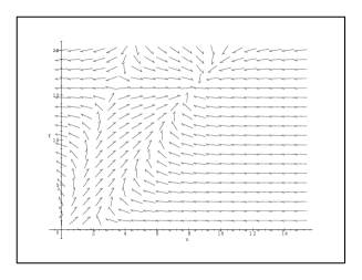
FIG. 2.: Flow diagram for $g^{*}=0.48$.

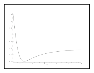
FIG. 3.: Plot of $\nu$ as a function of $g^{*}$ for $g^{*}\geq 0.42$

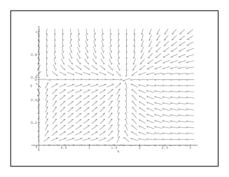
FIG. 4.: Flow diagram for the non-topological model.

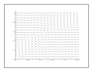
FIG. 5.: Detail of Fig.4 in the region near the tricritical line.

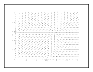
FIG. 6.: Flow diagram for the topological model with improved 1-loop calculations for $g^{*}=0.48$.

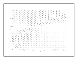
FIG. 7.: Detail of Fig.6 in the region near the tricritical line.

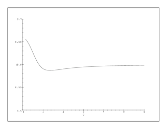
FIG. 8.: Plot of the exponent $\nu$ as a function of $g^{*}$.

REFERENCES

- [1] V. L. Ginzburg and L. D. Landau, Zh. Eksp. Teor. Fiz. 20, 1064 (1950).
- [2] J. Zinn-Justin, Quantum Field Theory and Critical Phenomena, 2nd edition (Oxford, 1993).
- [3] P. G. de Gennes, The Physics of Liquid Crystals, Oxford Univ. Press (1974).
- [4] B. I. Halperin, T. C. Lubensky and S.-K. Ma, Phys. Rev. Lett. 32, 292 (1974); J.-H. Chen, T. C. Lubensky and D. R. Nelson, Phys. Rev. B 17, 4274 (1978).
- [5] S. Hikami, Prog. Theor. Phys. 62, 226 (1979); I. D. Lawrie, Nucl. Phys. B 200 [FS 14] 1 (1982); Kolnberger and R. Folk, Phys. Rev. B 41, 4083 (1990); R. Folk and Y. Holovatch, J. Phys. A 29, 3409 (1996).
- [6] M. A. Aminisov, P. E. Cladis, E. E. Gorodetskii, D. A. Huse, V. E. Podnecks, V. G. Taratuta, W. van Saarlos and V. Voronov, Phys. Rev. A 41, 6749 (1990) and references therein.
- [7] C. Dasgupta and B. I. Halperin, Phys. Rev. Lett. 47, 1556 (1981).
- [8] M. Kiometzis, H. Kleinert and A. M. J. Schakel, Phys. Rev. Lett. 73, 1975 (1994).
- [9] I. F. Herbut, J. Phys. A 30, 423 (1997).
- [10] B. Bergerhoff, F. Freire, D. F. Litim, S. Lola and C. Wetterich, Phys. Rev. B 53, 5734 (1996).
- [11] I. F. Herbut and Z. Tesanović, Phys. Rev. Lett. 76, 4588 (1996); I. D. Lawrie, Phys. Rev. Lett., 78, 979 (1997); I. F. Herbut and Z. Tesanović, Phys. Rev. Lett. 78, 980 (1997).
- [12] K. G. Wilson And J. B. Kogut, Phys. Rep. 12, 75 (1974).
- [13] F. J. Wegner and A. Houghton, Phys. Rev. A 8, 401 (1975); J. Polchinski, Nucl. Phys. B 231, 269 (1984); C. Wetterich, Phys. Lett. B 301, 90 (1993); T. Morris, Int. J. Mod. Phys. A 9, 2411 (1994).
- [14] M. Reuter and C. Wetterich, Nucl. Phys. B 427, 291 (1994); U. Ellwanger, M. Hirsch and A. Weber, Z. Phys. C 69, 687 (1996); F. Freire and C. Wetterich, Phys. Lett. B 380, 337 (1996); M. D’Attanasio and T. Morris, Phys. Lett. B 378, 213 (1996).
- [15] L. Radzihovsky, Europhys. Lett. 29, 227 (1995).
- [16] A. P. C. Malbouisson, F. S. Nogueira and N. F. Svaiter, Europhys. Lett. 41, 547 (1998).
- [17] H. Kleinert and A. M. J. Schakel, Freie University preprint (1993).
- [18] G. W. Semenoff, P. Sodano and Y.-S. Wu, Phys. Rev. Lett. 62, 715 (1989); S. H. Park, Phys. Rev. D 45, R3332 (1992); Mod. Phys. Lett. A 7, 1579 (1992); G. Ferretti and S. G. Rajeev, Mod. Phys. Lett. A 7, 2087 (1992); P.-N. Tan, B. Tekin and Y. Hosotani, hep-th/9703121.
- [19] I. D. Lawrie, Phys. Rev. B 50, 9456 (1994); Phys. Rev. Lett. 72, 3238 (1994).
- [20] J. Bartholomew, Phys. Rev. B 28, 5378 (1983).
- [21] H. Kleinert, Lett. Nuovo Cimento 35, 405 (1982).
- [22] We thank Z. Tesanovic for this observation.
- [23] A. B. Harris, R. D. Kamien and T. C. Lubensky, Phys. Rev. Lett. 78, 1476 (1997); T. C. Lubensky, A. B. Harris, R. D. Kamien and Gu Yan, cond-mat/9710349.
- [24] X. G. Wen, F. Wilczek and A. Zee, Phys. Rev. B 39, 11413 (1989).
- [25] For a review see E. Fradkin, Field Theories of Condensed Matter Systems, Addison-Wesley, 1991.