Electronic topological transition in 2D electron system on a square lattice and the line $T^{*}(\delta)$ in the underdoped regime of high-$T_{c}$ cuprates

Abstract

It is shown that a 2D system of free fermions on a square lattice with hoping between more than nearest neighbours undergoes a fundamental electronic topological transition (ETT) at some electron concentration $n_{c}$. The point $\delta=\delta_{c}$, $T=0$ ($\delta=1-n$) is an exotic quantum critical point with several aspects of criticality. The first trivial one is related to singularities in thermodynamic properties. An untrivial and never considered aspect is related to the effect of Kohn singularity (KS) in 2D system : this point is the end of a critical line $T=0$, $\delta>\delta_{c}$ of static KS in free fermion polarizability. This ETT is a motor for anomalous behaviour in the system of interacting electrons. The anomalies take place on one side of ETT, $\delta<\delta_{c}$, and have a striking similarity with the anomalies in the high $T_{c}$ cuprates in the underdoped regime. The most important consequence of ETT is the appearance of the line of characteristic temperatures, $T^{*}(\delta)\propto\delta_{c}-\delta$, which grows from the point $\delta=\delta_{c}$ on the side $\delta<\delta_{c}$. Below this line the metal state is anomalous. Some anomalies are considered in the present paper. The anomalies disappear in the case $t^{\prime}=t^{\prime\prime}=...\rightarrow 0$.

flo1

style_def anomal expr p = cdraw p; cfill (tarrow (p, .55)); cfill (harrow (p, .55)); enddef; style_def wiggly_arrow expr p = cdraw (wiggly p); shrink (2); cfill (arrow p); endshrink; enddef;

I Introduction

Many experiments performed for high $T_{c}$ cuprates provide an evidence for unusual behaviour in the underdoped regime. Analysis of NMR [1, 2], angular photoemission study [3], infrared conductivity [4], transport properties [5], thermopower [6], heat capacity [7], spin susceptibility [8] and Raman spectroscopy [9] have revealed the existence of a characteristic energy scale $T^{*}(\delta)$ in the normal state with an absolute value different for different properties while universal feature is increase of $T^{*}(\delta)$ with decreasing doping.

We don’t know any theory which predicts the existence of such a line apart from theories containing only different hypothesis not explicit calculations.

With this paper we start a series of articles in which firstly we show the existence of such a line in 2D system of electrons on a square lattice with hoping between more than nearest neighbours and analyse its origin and then we demonstrate its appearance for different properties. In the present paper we consider only the origin of the line and its appearance in magnetic properties : SDW correlation length, NMR and neutron scattering. Electronic properties are considered in [10, 11]. Transport properties are currently under study.

We show that when varying the electron concentration defined as $1-\delta$, the system of noninteracting electrons on a square lattice undergoes an electronic topological transition (ETT) at a critical value $\delta=\delta_{c}$. The corresponding quantum critical point (QCP) has a triple nature. The first aspect of the criticality is related to the local change in FS at $\delta=\delta_{c}$. It leads to divergences in the thermodynamic properties, in the density of states at $\omega=0$ (the Van Hove logarithmic singularity [12]), in the ferromagnetic (FM) response function and to the additional divergence in the superconducting (SC) response function of noninteracting electrons. This induces FM and SC instabilities in the vicinity of QCP in the presence of the interactions of necessary signs.

The second aspect is related to the topological change in mutual properties of the FS in the vicinities of two different SP’s and leads to the logarithmic divergence of spin density and charge density susceptibilities of noninteracting electrons. This divergence has an ”excitonic” nature in the sense that the topology of two electron bands around two different SP’s is such that no energy is needed to excite an electron-hole pair. This can lead to spin-density wave (SDW) or charge-density wave (CDW) instability in the presence of the corresponding interaction.

The change in mutual topology of FS around SP’s is also responsible for the third aspect of the criticality related to the fact that this point is the end of a critical line of static Kohn singularities in the density-density susceptibility which exists only on one side of QCP, $\delta>\delta_{c}$. [What we mean as the static Kohn singularity is a square-root singularity at $\omega=0$ and wavevector ${\bf q}_{m}$ which connects two points of Fermi surface (FS) with parallel tangents [14, 15, 16]. For an isotropic FS and for 1D case this wavevector is nothing but ”$2k_{F}$”.]

The latter aspect of criticality exists only in the case of finite $t^{\prime}$ or/and $t^{\prime\prime}$ etc. (where $t^{\prime}$, $t^{\prime\prime}$ are hoping parameters for next nearest, next next nearest neighbors etc.) and has never been considered [17] However as we show in the present paper it is just this aspect that leads to numerous anomalies in the 2D electron system on the other side of QCP, $\delta<\delta_{c}$ which have a striking similarity with the anomalies in the high $T_{c}$ cuprates in the underdoped regime and are in our opinion at the origin of the latter anomalies.

The system of nonineracting electrons is considered in Sec.II. We demonstrate the existence of ETT for the case of electrons on a square lattice with $t$ and $t^{\prime}$ hoping parameters and discuss its different aspects. ETT firstly has been considered by I. Lifshitz [18] for 3D metals. It was shown that ETT implies an anomalous behavior and singularities in the thermodynamic and kinetic properties close to the transition point [19]. We show that for the 2D system the anomalies are still there but the situation is different and much more rich. We study the behaviour of density-density susceptibility and show that it behaves qualitatively different on two sides of ETT : quite ordinary on one side, $\delta>\delta_{c}$, and anomalously on the other, $\delta<\delta_{c}$. We discover the existence of a line $T^{*}(\delta)\propto\delta_{c}-\delta$ of Kohn anomalies which grows from the QCP on the side $\delta<\delta_{c}$. These anomalies are related to dynamic Kohn singularities at $T=0$.

The anomalies in the system of noninteracting electrons are at the origin of anomalies which appear in the presence of interaction, see Sec.III. Dependently on the type of interaction, CDW or SDW instability takes place around QCP. We consider a spin-dependent interaction of the AF sign and respectively the SDW phase. Strange about this phase is that the critical line has an unusual shape as a function of $\delta$ in the regime $\delta<\delta_{c}$ : It increases with increasing the distance from QCP instead of having the form of a ”bell” around QCP as it is usually happens for an ordered phase developing around an ordinary quantum critical point and as indeed it occurs on the side $\delta>\delta_{c}$. The reason is that the ordered phase develops rather ”around” the line $T^{*}(\delta)$ than around the quantum critical point at $T=0,Z=0$. We call this instability the SDW ”excitonic” instability in order to distinguish it from the SDW instability associated with nesting of Fermi surface occuring in the case $t^{\prime}=t^{\prime\prime}=...0$. In the latter case all anomalies discovered in the paper disappear. The reason is discussed in [20].

The line $T^{*}(\delta)$ plays a very important role also for the disordered metallic state out of the SDW ”excitonic” ordered phase. We show that it is a line of almost phase transition. The correlation length increases when approaching this line at fixed doping from high and from low temperature, relaxation processes slow down etc.

The metallic state below the line $T^{*}(\delta)$ is quite strange. On one hand, it exhibits a reentrant behaviour becoming more rigid with increasing temperature. On the other hand, dependences of the correlation length and of the parameter $\kappa^{2}_{exc}$ (which describes a proximity to the ordered SDW ”excitonic” phase) on doping are extremely weak. It leads to the unusual behaviour : in this regime the system remains effectively in a proximity of the ordered SDW phase for all dopind levels even quite far from $\delta_{exc}(T=0)$. Therefore the metallic state below the line $T^{*}(\delta)$ and out of the ordered SDW ”excitonic” phase is a reentrant in temperature and almost frozen in doping rigid SDW liquid. This state is characterized by numerous anomalies, some of them are considered in the paper. The existence of this state frozen in doping has very important consequences when considering the situation in the presence of SC phase. Since the line $T=T^{*}(\delta)$ is always leaning out of the SC phase, the normal state at $T_{sc}(\delta)<T<T^{*}(\delta)$ is quite strange : Being located in a proximity of the SC phase in fact it keeps a memory about the SDW ”excitonic” phase. It is this feature which on our opinion is crucial for understanding the anomalous behaviour in the underdoped regime of high-$T_{c}$ cuprates.

In the end of the Sec.III we discuss briefly an anomalous behaviour of physical characteristics corresponding to those measured by NMR and inelastic neutron scattering (INS). The discovered anomalies are in a good agreement with nuclear spin lattice relaxation rate $1/T_{1}T$ and nuclear transverse relaxation rate $1/T_{2G}$ experimental data on copper (see for example [2]). We discuss also a possible reason for the different behaviour of $1/T_{1}T$ on copper and oxygen [21]. We do some predictions for INS which can be verified by performing an energy scan in the normal state in a progressive change of temperature. More detailed analysis of the behaviour of $Im\chi({\bf q},\omega)$ measured by INS is performed in [22]. The Sec.IV contains summary and discussion.

II Quantum critical point and electronic topological transition in a system of noninteracting 2D electrons

Let us consider noninteracting electrons on a quadratic lattice with nn and nnn hopping. The dispersion law is written as

$$\epsilon_{{\bf k}\sigma}=\ -2t(cosk_{x}+cosk_{y})-4t^{\prime}cosk_{x}cosk_{y}\$$ (1)

where $t$ and $t^{\prime}$ are hoping parameters for nearest and next nearest neighbors. We consider $t>0$ and $t^{\prime}<0$ in order to correspond to the experimental situation which reveals the open FS in the underdoped regime. The dispersion (1) is characterized by 2 different saddle points (SP’s) located at $(\pm\ \pi,0)$ and $(0,\pm\pi)$ (in the first Brillouin zone $(-\pi,0)$ is equivalent to $(\pi,0)$ and $(0,-\pi)$ is equivalent to $(0,\pi)$) with the energy

$$\epsilon_{s}=4t^{\prime}.$$ (2)

When we vary the chemical potential $\mu$ or the energy distance from the SP, $Z$, determined as

$$Z=\mu-\epsilon_{s}-=\epsilon_{F}-4t^{\prime},$$ (3)

the topology of the Fermi surface changes when $Z$ goes from $Z<0$ to $Z>0$ through the critical value $Z=0$. In the first Brillouin zone, the Fermi surface is closed for $Z<0$ and open for $Z>0$. When $Z$ initially negative goes positive there is formation of two necks at ${\bf k}=(0,\pi)$ and ${\bf k}=(\pi,0)$. When the Brillouin zone is extended, the Fermi surface goes from convex ($Z<0$) to concave ($Z>0$), see Fig.1.

FIG. 1.: Fermi surface of the electron system with the dispersion law (1) for different Z and $t^{\prime}/t=-0.3$. The thick line corresponds to $Z=0$. Here $\tilde{k}_{x}=k_{x}/\pi$, $\tilde{k}_{y}=k_{y}/\pi$

The point $T=0,Z=0$ corresponds to an ELECTRONIC TOPOLOGICAL TRANSITION (ETT). It is a quantum critical point (QCP) which has a triple nature.

A Three aspects of criticality of the point $Z=0$, $T=0$

1. The first aspect of criticality is related to properties of one SP, i.e. to the local change in topology of FS in the vicinity of SP. It results in singularities in thermodynamical properties, in FM response function, in density of states at $\omega=0$, in additional (with respect to usual metal) singularity in SC response function.

The thermodynamical and FM singularities are given by

$$\delta G\propto Z^{\frac{d+2}{2}},\hskip 17.07182pt\frac{C}{T}=\frac{d^{2}\delta G}{dT^{2}}\propto\ lnZ,\hskip 17.07182pt\chi=\frac{d^{2}\delta G}{dh^{2}}\propto\ lnZ$$ (4)

as $T\rightarrow 0$ and by

$$\delta G\propto T^{\frac{d+2}{2}},\hskip 17.07182pt\frac{C}{T}=\frac{d^{2}\delta G}{dT^{2}}\propto\ lnT,\hskip 17.07182pt\chi=\frac{d^{2}\delta G}{dh^{2}}\propto\ lnT$$ (5)

as $Z\rightarrow 0$ (d is dimension, $G$ is the Gibbs potential, $C$ is heat capacity, $\chi$ is uniform susceptibility; the expressions for $\frac{C}{T}$ and $\chi$ are given for $d=2$) [More generally the singularities in the thermodynamic properties are described by the expression $\delta G\propto Z^{(d+z)\nu}F(\frac{T}{Z^{\nu z}})$ with $z=2$, $\nu=1/2$ ( a gaussian type behaviour). We will discuss this elsewhere.]

The SC response function for noninteracting electrons is related to the Green function

$$G_{sc}^{0}({\bf k},i\omega_{n})=-T\sum_{{\bf q},\omega_{m}}K_{i}({\bf q},i\omega_{m})K_{i}({\bf k-q},i\omega_{n-m})$$ (6)

and is given by

$${\sf\Pi}^{0}({\bf k},\omega)=-\lim_{\delta\rightarrow 0}G^{0}_{sc}({\bf k},\omega+i\delta)=\frac{1}{N}\sum_{{\bf q}}\frac{1-n^{F}(\tilde{\epsilon}_{{\bf q}})-n^{F}(\tilde{\epsilon}_{{\bf{q+k}}})}{\tilde{\epsilon}_{\bf q}+\tilde{\epsilon}_{\bf q+k}-\omega-i0^{+}}.$$ (7)

It diverges double logarithmically as a function of $T$ as ${\bf k}\rightarrow 0$, $\omega\rightarrow 0$ and $Z=0$ :

$${\sf\Pi}^{0}({\bf k}=0,\omega=0)\propto\ln^{2}T$$ (8)

When $T\rightarrow 0$ and $Z\rightarrow 0$ it diverges as

$${\sf\Pi}^{0}({\bf k}=0,\omega=0)\propto N(Z)\ln{\frac{\omega_{max}}{T}}\propto\ln{\frac{\omega_{max}}{T}}\ln{\frac{\omega_{max}}{|Z|}}.$$ (9)

where $N(Z)$ is the density of states.

2. The second aspect is related to mutual properties of two different SP’s and reveals itself when considering the density-density susceptibility (or by other words the electron-hole response function) at ${\bf k=Q}_{AF}=(\pi,\pi)$, i.e. at the wavevector which joins two SP’s. This response function is related to the electron-hole Green function of noninteracting electrons

$$G_{e-h}^{0}({\bf p},i\omega_{n})=-T\sum_{{\bf q},\omega_{m}}K_{1}({\bf q},i\omega_{m})K_{2}({\bf p+q},i\omega_{n+m})$$ (10)

and is given by

$$\chi^{0}({\bf k},\omega)=-\lim_{\delta\rightarrow 0}G^{0}_{e-h}({\bf k+Q}_{AF},\omega+i\delta)=\frac{1}{N}\sum_{{\bf q}}\frac{n^{F}(\tilde{\epsilon}_{{\bf q}})-n^{F}(\tilde{\epsilon}_{{\bf{q+k}}})}{\tilde{\epsilon}_{{\bf q+k}}-\tilde{\epsilon}_{{\bf{q}}}-\omega-i0^{+}}.$$ (11)

It diverges logarithmically as ${\bf k}\rightarrow{\bf Q}_{AF}$, $\omega\rightarrow 0$ and $Z=0$ :

$$\chi^{0}({\bf Q}_{AF},0)\propto\ln\frac{\omega_{max}}{T},$$ (12)

and as ${\bf k}\rightarrow{\bf Q}_{AF}$, $\omega\rightarrow 0$, $T=0$ :

$$\chi^{0}({\bf Q}_{AF},0)\propto\ln\frac{\omega_{max}}{|Z|}.$$ (13)

The one-electron Green functions $K_{i}({\bf k},\omega_{n})$ in (6), (10) are defined as

$$K_{i}({\bf k},\omega_{n})=\frac{1}{i\omega_{n}-\tilde{\epsilon}_{i}({\bf k})}$$ (14)

where $\tilde{\epsilon}_{1}({\bf k})=\epsilon_{1}({\bf k})-\mu$ and $\tilde{\epsilon}_{2}({\bf k})=\epsilon_{2}({\bf k})-\mu$ are the electron spectra in the vicinity of two different SP’s :

$$\tilde{\epsilon}_{1}(\bf k)=\tilde{\epsilon}(\bf k),$$

$$\tilde{\epsilon}_{2}({\bf k})=\tilde{\epsilon}({\bf k+Q}_{AF}),$$ (15)

and $\epsilon(\bf k)$ is determined by (1) (here and below we omitt the index $\sigma$ in the electron spectrum due to its degeneracy). In the hyperbolic approximation one has

$$\tilde{\epsilon}_{1}({\bf k})/t=-Z/t+ak_{x}^{2}-bk_{y}^{2},\hskip 28.45274pt(a=1-2t^{\prime}/t,\hskip 8.5359ptb=1+2t^{\prime}/t)$$

$$\hskip-128.0374pt\tilde{\epsilon}_{2}({\bf k})/t=-Z/t+a(k^{\prime}_{y})^{2}-b(k^{\prime}_{x})^{2},$$ (16)

where the vawevectors $k_{x}$, $k_{y}$ are defined as the deviations from the SP wavevector $(0,\pi)$ and the vawevectors $k^{\prime}_{x}$, $k^{\prime}_{y}$ as the deviations from the SP wavevector $(\pi,0)$.

The divergences (12), (13) have an ”excitonic” nature [23] and this is the second aspect of the criticality of the considered QCP. What we mean as the ”excitonic” nature is that the chemical potential lies on the bottom of one ”band” (around one SP) and on the top of the another (around another SP) for the given directions $(0,\pi)-(\pi,\pi)$ and $(\pi,0)-(0,0)$, see Fig.2. Therefore, no energy is needed to excite the electron-hole pair.

FIG. 2.: Schematical presentation of the electron spectrum in a vicinity of two SP’s for $Z=0$.

3. The third aspect of the criticality is related to the fact that this point is the end of a critical line of the static square-root Kohn singularities in $\chi^{0}({\bf q},\omega)$. It is this aspect which gives rise to asymmetrical behaviour of the system on two sides of QCP, $Z<0$ and $Z>0$ and to other anomalies. Below we will concentrate on this aspect of criticality as has never been considered before.

B The line of static Kohn singularities in the vicinity of ${\bf q}={\bf Q}_{AF}$ for $T=0$, $Z<0$

One can show by simple calculations that for each point of demiaxis $Z<0$ there is a vavevector ${\bf q=q}_{m}$ in a vicinity of ${\bf Q}_{AF}$ (in each direction around ${\bf Q}_{AF}$) such that

$$Re\chi^{0}({\bf q},0)-Re\chi^{0}({\bf q}_{m},0)=\left\{\begin{array}[]{cc}A\sqrt{|{\bf q}_{m}-{\bf q}|},&\hskip 8.5359pt{\bf q}<{\bf q}_{m},\\ B|{\bf q}-{\bf q}_{m}|,&\hskip 8.5359pt{\bf q}>{\bf q}_{m}.\end{array}\right.$$ (17)

This is a static Kohn singularitiy in the 2D electron system. The absolute value of this wavevector in the given direction $\phi$, $Q_{m}(\phi)=|{\bf Q}_{AF}-{\bf q}_{m}(\phi)|$, is proportional to the square-root of the energy distance from QCP :

$$Q_{m}(\phi)\propto\sqrt{\mid Z\mid}.$$ (18)

Therefore for each fixed negative $Z$ one has a closed line of the static Kohn singularities around ${\bf q=Q}_{AF}$. With decreasing $|Z|$ the close line shrinks and is ended at $Z=0$ being reduced to the point ${\bf q=Q}_{AF}$. The closed line of the static Kohn singularities does not grow again on the other side of QCP, $Z>0$.

To illustrate this we show in Fig.3 the wavevector dependences of $\chi^{0}({\bf k},0)$ calculated based on (11) and (1). In these plots one sees only a quarter of the picture around ${\bf q=Q}_{AF}$; to see the closed line of square shape around ${\bf Q}_{AF}$ one has to consider the extended BZ around $(\pi,\pi)$.

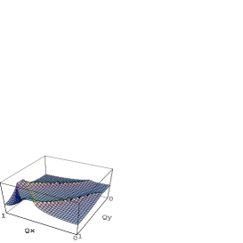
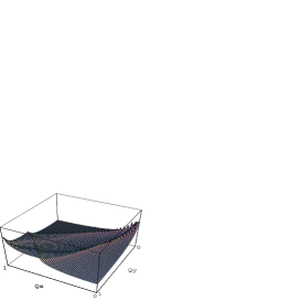
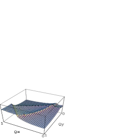
a)                                            b)                                           c)

FIG. 3.: Wavevector dependences of the static susceptibility $\chi^{0}({\bf q},0)$ for (a) $Z<0$, (b) $Z=0$ and (c) $Z>0$ ($t^{\prime}/t=-0.3$). Here $Q_{x}=q_{x}/\pi$, $Q_{y}=q_{y}/\pi$. The point ${\bf q=Q}$ corresponds to the left corner.

The discussed above line is the closest to ${\bf Q}_{AF}$ line of singularities in Fig.3a. [There are few other lines of the Kohn singularities seen in Fig.3 which are not sensitive to ETT, we discuss them in [20]] One can see that this line disappears at $Z=0$ and does not reappear at $Z>0$ (while the other lines of Kohn singularities in a proximity of ${\bf Q}_{AF}$ do not change across QCP).

The wavevector dependence of the static susceptibility in the regime $Z>0$ has a weak maximum at ${\bf q=Q}_{AF}$ for very small values of $Z$, for higher $Z$ it exhibits a wide plateau until some border wavevector whose value for a given direction depends on $Z$ only slightly, see Fig.4. To illustrate an evolution with $Z$ of the $\bf q$ dependence of $\chi^{0}({\bf q},0)$ for both regimes we present in Fig.4 calculations of $\chi^{0}({\bf q},0)$ in the fixed direction, here $(q_{x},\pi)$

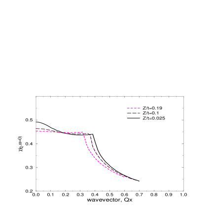
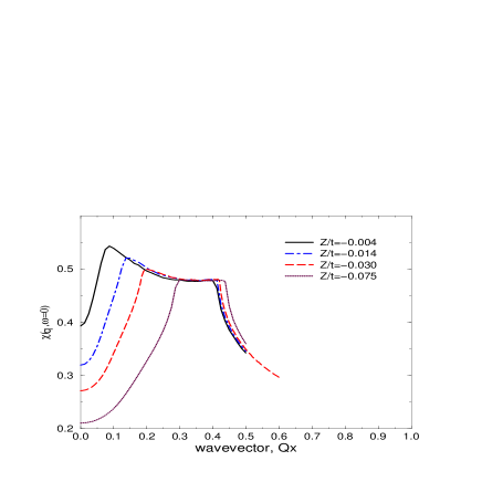
a)                                                     b)

FIG. 4.: Static susceptibility $\chi^{0}({\bf q},0)$ as a function of wavevector in the direction $(q_{x},\pi)$ for different values of $Z$ in the cases $Z>0$ (a) and $Z<0$ (b). $t^{\prime}/t=-0.3$). Here $Q_{x}=(\pi-q_{x})/\pi$.

The difference between behaviour on two sides of QCP is clear : there is incommensurability (singularity) on one side and commensurability on the other. In both cases there is a singularity at rather high wavevector $Q_{x}$ whose origin we discuss in [20].

It is important to know for the following applications how the plateau in the regime $Z>0$ evolves with $T$. For this we show in Fig.5 the $\bf q$ dependence of $Re\chi^{0}$ calculated for fixed $Z$ and increasing $T$.

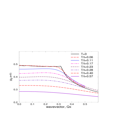
FIG. 5.: Static electron-hole susceptibility $\chi_{0}({\bf q},0)$ as a function of wavevector in the direction $(q_{x},\pi)$ for $Z/t=0.19$ and different temperature ($t^{\prime}/t=-0.3$)

One can see that the plateau survives until very high temperature.

Above we analyzed the $\bf q$ dependence of the electron-hole susceptibility on the critical line $T=0$, $Z<0$ ($\omega=0$). It is also worth to know the type of singularities in $T$ and $\omega$ for the susceptibility $\chi^{0}({\bf q}_{m},Z,\omega,T)$ when approaching the critical line. They are given by :

$$\chi^{0}({\bf q}_{m},Z,\omega,T)-\chi^{0}({\bf q}_{m},Z,\omega=0,T=0)\propto\sqrt{T-i\omega},\hskip 28.45274ptT\rightarrow 0,\omega\rightarrow 0$$ (19)

for finite $Z$ ($Z>T$, $Z>\omega$). When approaching the end of the critical line which is the ETT quantum critical point $T=0$, $Z=0$ ($\omega=0$), the behaviour changes. Now it depends on the order $Z\rightarrow 0$ and $T\rightarrow 0$, $\omega\rightarrow 0$. When first $T\rightarrow 0$, $\omega\rightarrow 0$ we still have eq. (19). When first $Z\rightarrow 0$ one has

$$\chi^{0}({\bf Q}_{AF},Z,\omega,T)\propto Ln(T+i\omega).$$ (20)

It was the static Kohn singularities which exist only on one side of QCP, $Z<0$, and take place for the incommensurate wavevector ${\bf q}={\bf q}_{m}$. Below we show that on the other side, $Z>0$, static singularities related to ETT do not exist but a dynamic Kohn singularity also related to ETT appears at ${\bf q}={\bf Q}_{AF}$.

C The line of dynamic Kohn singularity for $T=0$, $Z>0$

Let’s analyse the energy dependence of $\chi^{0}({\bf q},\omega)$ in the regime $Z>0$ for the characteristic wavevector in this regime, ${\bf q}={\bf Q}_{AF}$. The calculated dependence (based on (11) and the full spectrum (1)) is shown in Fig.6. One can see that for fixed $Z$ there is a characteristic energy, $\omega_{c}$, where $Im\chi^{0}$ and $Re\chi^{0}$ are singular. This energy increases with increasing $Z$. There is a plateau in $Re\chi^{0}$ for $\omega<\omega_{c}$ and a sharp decrease for $\omega>\omega_{c}$. As this behaviour has very important consequences, we are going to analyse it analytically.

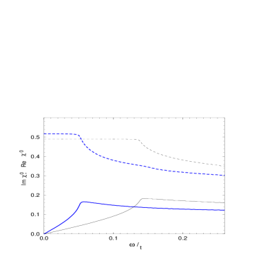
FIG. 6.: Energy dependences of $Re\chi^{0}$ (dashed lines) and $Im\chi^{0}$ (solid lines) for the wavevector ${\bf q}={\bf Q}_{AF}$. The thick lines correspond to $Z/t=0.04$, the thin lines to $Z/t=0.1$ ($t/t^{\prime}=-0.3$).

Calculations of $Im\chi^{0}({\bf k},\omega)$ for ${\bf k}={\bf Q}_{AF}$ performed with the hyperbolic spectrum (16) give the scaling expression

$$Im\chi^{0}({\bf Q}_{AF},\omega)=\frac{1}{2\pi t}F(\frac{\omega}{\omega_{c}},\frac{b}{a}),$$ (21)

where the scaling function $F(x,y)$ is determined as follows

$$F(x,y)=\left\{\begin{array}[]{cc}\ln{\frac{\sqrt{1+xy}+\sqrt{1+x}}{\sqrt{1-xy}+\sqrt{1-x}}},&0\leq x\leq 1\\ \ln{\frac{\sqrt{1+xy}+\sqrt{1+x}}{\sqrt{x(1-y)}}},&x\geq 1.\end{array}\right.$$ (22)

In (21), $a$ and $b$ are the coefficients of the dispersion law (16), $b/a$ is equal

$$b/a=1+\frac{4t^{\prime}/t}{1-2t^{\prime}/t}.$$

and $\omega_{c}$ is given by

$$\omega_{c}=\frac{2Z}{1-2t^{\prime}/t}.$$ (23)

[The expression (22) is valid for $t^{\prime}\neq 0$].

Using Kramers-Kronig relation one obtains the following equations for $Re\chi^{0}$ :

$$tRe\chi^{0}({\bf Q}_{AF},\omega)=tRe\chi^{0}({\bf Q}_{AF},\omega_{c})-\Phi(\frac{\omega}{\omega_{c}},\frac{b}{a}),$$ (24)

$$tRe\chi^{0}({\bf Q}_{AF},\omega_{c})=-\alpha\ln{(\omega_{c}/t)}+\beta.$$

In (24) $\alpha$ is given by

$$\alpha=F(\infty,b/a)/\pi^{2}=\frac{1}{\pi^{2}}\ln{(\frac{1+\sqrt{1-4(t^{\prime}/t)^{2}}}{1-\sqrt{1-4(t^{\prime}/t)^{2}}})}$$ (25)

and the asymptotic form of $\Phi(x,y)$ as a function of $x$ for fixed $y$ is given by :

$$\Phi(x,y)=\left\{\begin{array}[]{cc}\gamma_{1}(1-x^{2}),&x-1<0\\ \gamma_{2}\sqrt{x-1},&0\leq x-1\ll 1\\ \alpha[\ln{\frac{(x-1)t}{\omega_{max}}}],&x-1>x^{*}\end{array}\right.$$ (26)

The eq. (24)-(26) are valid for $Z/t<10^{-1}$. $\omega_{max}$ is a cutoff energy. The coefficients $\beta,\gamma_{1}$ and $\gamma_{2}$ depend on $t^{\prime}/t$. The analytical expressions are given in [10]. For example for $t^{\prime}/t=-0.3$ they are equal to : $\beta=0.218$, $\gamma_{1}\approx 10^{-2}$, $\gamma_{2}=0.18$. The value of $x^{*}$ is given by $x^{*}\approx 10$. The important features of $Re\chi^{0}$ are: (i) the almost perfect plateau for $\omega<\omega_{c}$ since $\gamma_{1}$ is extremely small (that is true for all finite $t^{\prime}/t$), (ii) the square-root singularity at $\omega=\omega_{c}$; (iii) the logarithmic behavior for large $\omega$ : $\omega>\omega^{*}\approx 10\omega_{c}$ (quantum critical behaviour).

Thus, we realize that the same root-square singularity in $Re\chi^{0}$ which exists in the regime $Z<0$ for ${\bf q}={\bf q}_{m}$ as $\omega\rightarrow 0^{+}$ (see eq.(19)) occurs in the regime $Z>0$ for ${\bf q}={\bf Q}_{AF}$ as $\omega\rightarrow\omega_{c}+0^{+}$. It is a dynamic 2D Kohn singularity. [We consider here only the case ${\bf q}={\bf Q}_{AF}$ since it is the wavevector where $\chi^{0}({\bf q},0)$ is maximum and which therefore determines all properties related to a long-range and short-range ordering. Dynamic Kohn singularities for ${\bf q}\neq{\bf Q}_{AF}$ will be discussed elsewhere]

It is worth to see how the dynamic Kohn singularities appear in 3D plot of $\chi_{0}({\bf Q}_{AF},\omega)$ as a function of $Z$ and of $\omega$. We show this in Fig.7a. If one plots the lines of Kohn singularities which end at QCP in $\omega-Z$ plane one gets a picture shown in Fig.7b which demonstrates the third aspect of the criticality of the considered QCP at $T=0$, $Z=0$.

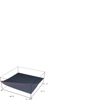
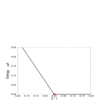
(a)                                                     (b)

FIG. 7.: The plots which demonstrate the third aspect of the criticality of QCP. (a) $Re\chi_{0}({\bf Q}_{AF},\omega)$ as a function of $Z$ and of $\omega$ in the regime $Z>0$, (b) two critical lines of Kohn singularities : $\omega=\omega_{c}^{-}=0$ for $Z<0$ and $\omega=\omega_{c}^{+}=\omega_{c}(Z)$ for $Z>0$. ($T=0$, $t^{\prime}/t=-0.2$)

In fact all properties related to $\chi_{0}({\bf Q}_{AF},\omega)$ are singular at the line $\omega=\omega_{c}(Z)$ not only $Re\chi_{0}({\bf Q}_{AF},0)$. In Fig.8 we show as an example the behaviour of another characteristics $C(\omega)=Im\chi^{0}({\bf Q}_{AF},\omega)/\omega$ as a function of $\omega$. [This characteristics we will use in the following sections to analyse NMR experimental data.]

FIG. 8.: Calculated $C(\omega)=Im\chi^{0}({\bf Q}_{AF},\omega)/\omega$ (solid line) as a function of $\omega$ for the regime $Z>0$ ($t^{\prime}/t=-0.3$, $Z/t=0.19$). For comparison we show also $Re\chi^{0}({\bf Q}_{AF},0)$ (dashed line)

One can see that a singularity takes place at the same energy as for $Re\chi_{0}({\bf Q}_{AF},0)$, i.e. at $\omega=\omega_{c}(Z)$. One can see also that $C$ is constant only at low energies, $\omega\ll\omega_{c}$ (Fermi-liquid behaviour). At higher energies it increases with $\omega$ until $\omega=\omega_{c}$, passes through the maximum at $\omega=\omega_{c}$ and then decreases. It is interesting to emphasize that except of very low $\omega$ such a behaviour gives an impression of the existence of a pseudogap in the one-electron spectrum although the pseudogap is absent in the bare electron spectrum.

D The lines of temperature ”Kohn anomalies” for $Z>0$

Let’s consider now the regime $Z>0$ for finite $T$, namely let’s consider a behaviour of $Re\chi^{0}({\bf Q}_{AF},0)$ as a function of $T$. Such dependences calculated for two different values of $Z$ are presented in Fig.9

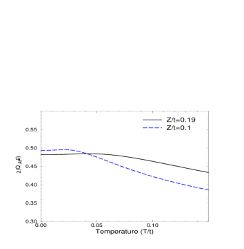
FIG. 9.: Static electron-hole susceptibility $\chi_{0}({\bf Q}_{AF},0)$ as a function of $T$ for two values of $Z$ in the regime $Z>0$ ($t^{\prime}/t=-0.3$).

When comparing with Fig.6 one can see that the behaviour is almost the same being of course smoothed by the effect of finite $T$ : there is a plateau until some temperature $T^{*}_{Re}$ and a rather sharp decrease at higher temperature. In the same way as it was for the characteristic energy, the characteristic temperature scales with $Z$ :

$$T^{*}_{Re}\propto Z.$$ (27)

In fact the behaviour of $Re\chi^{0}({\bf Q}_{AF},0)$ is slightly different from the plateau behaviour in the range $T<T^{*}_{Re}$. There is a slight maximum at the end of the ”plateau”. It is almost invisible in the graph but is quite important and intrinsic property : this maximum clearly distinguishes the point $T^{*}_{Re}$ which is the point of the temperature ”Kohn anomaly” and therefore the line $T^{*}_{Re}(Z)$ is the line of Kohn anomalies for $Re\chi^{0}$.

There is a much more pronounced maximum in $Z$ dependence of $Re\chi^{0}({\bf Q}_{AF},0)$ at finite $T$ and $Z>0$, see Fig.10. The position of the maximum is proportional to $T$, $Z^{*}_{Re}\propto T$. The point $Z^{*}_{Re}$ is the point of the electron concentration Kohn anomaly [24].

Another feature important for following applications is that $\chi_{0}({\bf Q}_{AF},0)$ as a function of $Z$ is assymetrical on two sides from $Z=Z^{*}$. On the side $Z>Z^{*}$ it depends on $Z$ very weakly and is practically constant starting from some threshold value of $Z-Z^{*}(T)$ (that is very unusual) while for $Z<Z^{*}$ it always decreases with increasing $|Z-Z^{*}(T)|$. The reason for the former behaviour is discussed in [20].

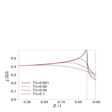
FIG. 10.: Static electron-hole susceptibility $\chi_{0}({\bf Q}_{AF},0)$ as a function of $Z$ for increasing $T$ ($t^{\prime}/t=-0.3$). The maximum at some $Z$ which we call $Z^{*}(T)$ is clearly seen.

It is useful to analyse lines of $Re\chi^{0}({\bf Q}_{AF},0)=const$ in the $T-Z$ plane which we present in Fig.11. These lines have a very unusual form which reflects the existence of the Kohn anomalies at $T^{*}_{Re}(Z)$, compare for example with the lines of the ordinary forms for the SC response function in Fig.15b. This will have an important consequence when we will take into account an interaction.

FIG. 11.: The lines of $Re\chi^{0}({\bf Q}_{AF},0)=const$ in the $T-Z$ plane for the regime $Z>0$.

Let’s analyse now the temperature dependence of $C(\omega)=Im\chi^{0}({\bf Q}_{AF},\omega)/\omega$ calculated in the limit $\omega\rightarrow 0$, see Fig.12. Its behaviour repeats in a smooth form the behaviour of $C(\omega)$ as a function of $\omega$ at $T=0$, see Fig.9. The important difference is that the characteristic temperatures for $Re\chi^{0}({\bf Q}_{AF},0)$ and $Im\chi^{0}({\bf Q}_{AF},\omega)/\omega$ are different on the contrary to the characteristic energy at $T=0$ which is the same for both $Re\chi^{0}$ and $Im\chi^{0}$. This is a usual effect of finite temperature. Of course both characteristic temperatures, $T^{*}_{Re}$ and $T^{*}_{Im}$ are proportional to $Z$ originating from the same effect of the Kohn singularities at $T=0$. It is important to note that $T^{*}_{Im}$ is always larger than $T^{*}_{Re}$.

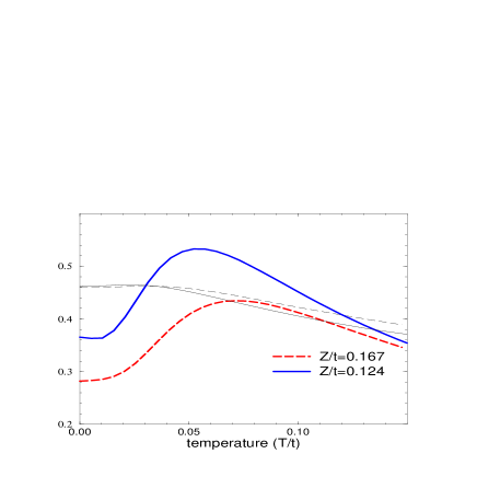
FIG. 12.: Temperature dependence of $C(\omega)=Im\chi^{0}({\bf Q}_{AF},\omega)/\omega$ in the limit $\omega\rightarrow 0$ for two values of $Z$ in the regime $Z>0$ (thick lines) ($t^{\prime}/t=-0.3$) (the existence of SC state is ignored). One can see that $C(0)$ remains constant until some temperature, $T_{F}$, (Fermi-liquid behaviour), then increases with $T$ and passes through the maximum at $T=T^{*}_{Im}(Z)$. For comparison we show also $Re\chi^{0}({\bf Q},0)$ for the same $Z$ (thin lines) which exhibits a weak maximum at $T=T^{*}_{Re}(Z)$.

If we plot the lines of the temperature Kohn anomalies $T^{*}_{Re}$ and $T^{*}_{Im}$ in the $T-Z$ plane we get a picture shown in Fig.13 which will be the reference picture for the system in the presence of interaction.

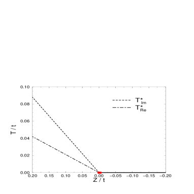
FIG. 13.: The lines of the temperature Kohn anomalies $T^{*}_{Re}$ and $T^{*}_{Im}$ ($t^{\prime}/t=-0.3$). We also show the critical line $T=0$, $Z<0$ (solid line)

It is worth to give one more example of the role of the lines $T^{*}(Z)$. In Fig.14a we show a temperature evolution of the $\omega$ dependence of $Re\chi^{0}({\bf Q}_{AF},\omega)$. The low energy plateau survives only until $T=T^{*}_{Re}$. The size of the plateau is :

$$\omega_{c}(Z,T)=\omega_{c}(Z,0)-a_{1}T$$ (28)

($a_{1}T^{*}_{Re}(Z)=\omega_{c}(Z,0)$). Above $T=T^{*}_{Re}$ the plateau disappears and the behaviour becomes ordinary. In Fig.14b we show a temperature evolution of the $\omega$ dependence of $C(\omega)$. The low energy increasing part survives only until $T=T^{*}_{Im}$. Above $T=T^{*}_{Im}$, the increasing part disappears

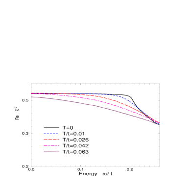
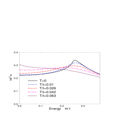
(a)                                            (b)

FIG. 14.: Evolution with temperature (a) of the plateau in $Re\chi^{0}({\bf Q},0)$ ($Z/t=0.17$, $T^{*}_{Re}/t=0.04$) and (b) of the increasing part in $C(\omega)$ ($Z/t=0.19$, $T^{*}_{Im}/t=0.05$). ($t^{\prime}/t=-0.3$)

The described above anomalous behaviour in the system of noninteracting electrons leads to very important consequences when taking into account an interaction.

E Superconducting polarization operator as a function of $Z$ and $T$

Before we start to consider the system in the presence of interaction it is worth to analyse the behaviour of the superconducting polarization operator $\Pi^{0}(0,0)$ as a function of $Z$ and of $T$. This behaviour is presented in Fig.15.

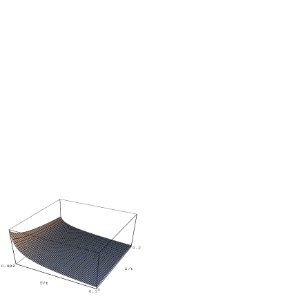
(a)                                            (b)

FIG. 15.: $\Pi^{0}(0,0)$ as a function of $Z$ and of $T$ (a) and lines of $\Pi^{0}(0,0)=const$ in $Z-T$ coordinates (b) for $Z>0$. The behaviour for $Z<0$ is totally symmetrical. The plot is started from $T=0.002$ since for $T=0$ there is a logarithmic divergence for any $Z$. ($t^{\prime}/t=-0.2$)

One can see that it is an ordinary behaviour as a function of $T$ for fixed $Z$ and as a function of $Z$ for fixed $T$ : $\Pi^{0}(0,0)$ decreases sharply as a function of $T$ for fixed $Z$ and as a function of $Z$ for fixed $T$. In fact the expressions (8), (9) work quite well for finite $T$ and $Z$ contrary to the case of $\chi^{0}({\bf Q}_{AF},0)$. This behaviour reflects the first aspect of the criticality of the considered QCP. We also present in Fig.15 the lines of $\Pi^{0}(0,0)=const$ in the $T-Z$ plane which have a quite ordinary monotonous form, compare with similar lines for $\chi^{0}({\bf Q}_{AF},0)$ in Fig.11.

It is worth to note that the same qualitatively behaviour takes place for the effective ”polarization operator” ${\sf\Pi}^{0}_{d}(0,0)$ determined as follows

$${\sf\Pi}^{0}_{d}(0,0)=\frac{1}{4}\sum_{\bf k}\frac{(\cos{k_{x}}-\cos{k_{y}})^{2}tanh(\frac{\tilde{\epsilon}({\bf k})}{2T})}{2\tilde{\epsilon}({\bf k})}.$$ (29)

It replaces the polarization operator $\Pi^{0}(0,0)$ in the case when the interaction responsible for the superconductivity is momentum dependent which leads to the d-wave symmetry of SC order parameter [25].

F A passage from the energy distance from QCP, $Z$, to the electron concentration

Above we have considered all properties as functions of the energy distance from the QCP. It is worth for applications to cuprates to change the description and to consider physical properties as functions of electron concentration $n_{e}$ or of hole doping $\delta=1-n_{e}$. To do such a passage we have to use a relation between $Z$ (or the chemical potential $\mu$) and the hole doping. To get this relation we will use the condition (for $T=0$) :

$$1-\delta=\frac{1}{N}\sum_{k\sigma}n^{F}(\epsilon_{{\bf k}\sigma}-\mu).$$ (30)

This condition corresponds to the electron FS with a volume $V_{e}\propto 1-\delta$. Experimentally observed in cuprates ”large” FS which exists in the metallic state even at quite low doping corresponds to the condition $V_{h}\propto 1+\delta$ which is equivalent to eq (30). On the other hand, as known, the undoped materials ($\delta=0$) correspond to a localized-spin AF state that demonstrates that the latter condition is certainly not correct for very low doping.

The problem of the volume of FS in cuprates, let say, $\delta$ versus $1+\delta$ (for the hole FS) is an independent problem which we do not want to discuss in details here. We would like to note only that we have reached some progress in the understanding of similar problem for the $t-J$ model [25] for which we have written (based on the diagrammatic technique for $X$-operators and using the first approximation in inverse number of nearest neighbours) an equation for the chemical potential as a function of doping [25]. We have shown that it is similar in a certain sense to the Van-der-Waals equation : in a certain interval of doping it has two ”physical” and one ”unphysical” solutions for each doping. Among ”physical” solutions one corresponds to the state with localized spins : electrons initially present (at $\delta=0$) are localized, FS is formed by doped holes only (Curie constant is constant as $T\rightarrow 0$, the volume of FS is proportional to $\delta$). This solution is unstable against AF ordering of localized-spin type. The second ”physical” solution corresponds to the state with all holes delocalized : the volume of FS is proportional to $1+\delta$ while the Curie constant tends to zero as $T\rightarrow 0$. In the case $t^{\prime}/t<0$ at low doping only solution of the former type exists while at high doping only the second one is possible. Postponing a quantitative analysis telling which phase is favorable at intermediate doping we presume (as a matter of fact for cuprates) that it is the second phase which is favorable and we consider at present only this state described at $T=0$ by the condition (30).

A value of the critical doping $\delta_{c}$ corresponding to the QCP at $Z=0$ is determined by the condition (30). It depends on value of $t^{\prime}/t$, see Fig.16.

FIG. 16.: Critical doping of ETT $\delta_{c}$ as a function of $t^{\prime}/t$. As realistic values for cuprates one gets for example, $\delta_{c}=0.17$ when $t^{\prime}/t=-0.2$, $\delta_{c}=0.27$ when $t^{\prime}/t=-0.3$. The value $t^{\prime}/t=-0.5$ is critical : the FS is degenerated into two lines.

So far as

$$Z\propto\delta_{c}-\delta,$$ (31)

all dependences considered above can be rewritten as functions of doping distance from QCP.

III The system in the presence of interaction

A Phase diagram

In the presence of interaction the expression for the electron-hole susceptibility in the simplest RPA approximation is given by

$$\chi({\bf q},\omega)=\frac{\chi^{0}({\bf q},\omega)}{1+V_{\bf q}\chi^{0}({\bf q},\omega)}.$$ (32)

The explicit form of the interaction depends on model. One can consider an interaction which leads to SDW or CDW instabilities or to both of them. For example, for the Hubbard model $V_{\bf q}=-U$, for the $t-J$ model $V_{\bf q}=J_{\bf q}$ ($J_{\bf q}=2J(\cos q_{x}+\cos q_{y})$). So far as both wavevectors ${\bf q}={\bf Q}_{AF}$ and ${\bf q}=0$ are critical for the considered QCP and $Re\chi^{0}({\bf q},0)$ diverges for both of them whereas experimentally for cuprates only a response around ${\bf q}={\bf Q}_{AF}$ is observed and it is a spin dependent response one should consider this as a phenomenological argument in a favour of the momentum dependent interaction in a triplet channel. From now on we shall mainly consider the case of cuprates and therefore we shall use $V_{\bf q}=J_{\bf q}$ with a positive sign, $J>0$.

The line of SDW instability associated with the considered QCP is given by

$$1/J_{\bf q}=-\chi^{0}({\bf q},0).$$ (33)

It is clear from the previous analysis that the instability occurs at ${\bf q}={\bf Q}_{AF}$ on the side $Z>0$ (or $\delta<\delta_{c}$) and close to ${\bf q}={\bf q}_{m}$ on the side $Z<0$ (or $\delta>\delta_{c}$). Below we will call this instability the SDW ”excitonic” instability in order to distinguish from the SDW instability associated with nesting of Fermi surface occuring in the case $t^{\prime}=0$. In the latter case all discussed in the paper anomalies originated from the dynamic Kohn singularities disappear: the behaviour of $\chi({\bf q},\omega)$ is symmetrical in $Z$ and corresponds to that in the regime $Z<0$ in the case $t^{\prime}\neq 0$. The reason is discussed in [20].

From Fig.11 which shows the lines of $Re\chi^{0}({\bf Q}_{AF},0)=const$ in $T-Z$ coordinates it is clear that the critical line $T_{exc}(Z)$ would have an unusual shape as a function of $Z$ in the regime $Z>0$. Indeed, we see in Fig.17 that $T_{exc}(Z)$ increases with increasing the distance from QCP instead of having the form of a ”bell jar” around QCP as it usually happens for an ordered phase developing around an ordinary quantum critical point and as indeed it occurs on the side $Z<0$ [26].

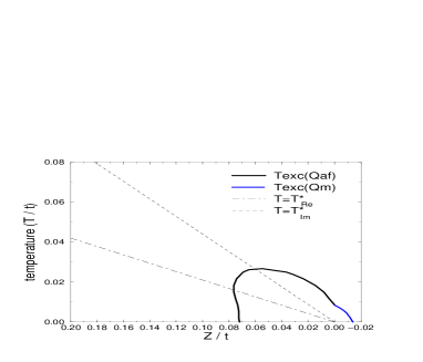
FIG. 17.: Phase diagram around QCP, $T=0$, $Z=0$. The solid line corresponds to the SDW ”excitonic” instability occuring at ${\bf q}={\bf Q}_{AF}$ in the regime, $Z>0$ and at the incommensurate wavevector ${\bf q}={\bf q}_{m}$ in the regime, $Z<0$. We show also the lines $T^{*}_{Re}(\delta)$ and $T^{*}_{Im}(\delta)$ discussed in the text. ($t/J=1.9$, $t^{\prime}/t=-0.3$)

The form of $T_{exc}(Z)$ reflects the fact that the SDW ”excitonic” ordered phase develops rather ”around” the line $T^{*}_{Re}(Z)$ than around the point $T=0,Z=0$.

On the contrary, the form of the critical line for the SC phase, $T_{sc}(Z)$, which develops around the considered QCP is very ordinary as it repeats the form of the lines in Fig.15.b Whatever is the nature of the interaction responsible for the existence of high $T_{c}$ superconductivity, the line $T_{sc}(Z)$ has the usual shape of ”bell” being symmetrical for the regimes $Z>0$ and $Z<0$ (or $\delta<\delta_{c}$ and $\delta>\delta_{c}$) which therefore we can call the underdoped and overdoped regimes, respectively. The ordinary form is related to the ordinary behaviour of $\Pi^{0}(0,0)$ and $\Pi_{d}^{0}(0,0)$ as a function of $Z$ and of $T$ as discussed in the Sec.II.E. We will not discuss details concerning the SC phase here (see [25] where the line of SC instability is discussed from below and [22] where it is discussed from above].

Anyway there are two possibilities : (i) the ordered SDW ”excitonic” phase leans out OF the SC phase as in Fig.18a, (ii) the ordered SDW ”excitonic” phase is completely hidden under the SC phase as in Fig.18b. It depends on the ratio $J/W$, where $W$ is a bandwidth of the electron band (detailed calculations for SC critical line are presented in [22]). [An interplay and a mutual influence of the two ordered phases, SDW ”excitonic” and SC, will be discusses elsewhere].

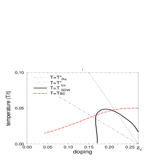
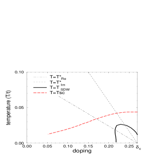
(a)                                            (b)

FIG. 18.: Phase diagram in coordinates $T-\delta$ with the lines of SDW ”excitonic” instability , SC instability and the lines $T^{*}_{Re}(\delta)$ and $T^{*}_{Im}(\delta)$ discussed in the text ($t^{\prime}/t=-0.3$, $t/J=1.8$ in (a) and $t/J=1.9$ in (b)). We show only the underdoped part of the phase diagram.

In both cases the lines $T^{*}_{Re}(\delta)$ and $T^{*}_{Im}(\delta)$ persist above $T_{sc}(\delta)$ in the underdoped regime and therefore it is worth to analyse properties of the normal state in the underdoped regime above and below these lines.

B Metallic state in the proximity of the ordered SDW ”excitonic” phase.

Below we consider some properties in the undistorted metallic state out of the ordered SDW ”excitonic” phase which are characterized by anomalous behaviour.

Taking into account the $\omega$ and $\bf q$-dependence of $Im\chi^{0}$ and $Re\chi^{0}$ given by (21)-(26) and the definition (32) one can present the electron-hole susceptibility describing fluctuations around ${\bf Q}_{AF}$ in a proximity of the SDW ”excitonic” phase in the form

$$\chi({\bf q},\omega)=\frac{1}{4J}(\frac{\alpha+iC\omega}{(1-\alpha)+A({\bf q-Q}_{AF})^{2}-iC\omega}),\hskip 28.45274pt\omega<\omega_{c}(T)$$ (34)

with $\alpha$ which is defined as

$$\alpha=4J\chi^{0}({\bf Q}_{AF},0)$$ (35)

and which is close to unity in THE proximity of the ordered phase. The form (34) is valid for $\bf q$ in the vicinity of ${\bf Q}_{AF}$ (${\bf Q}_{AF}-{\bf q}\ll 1$) and for $\omega<\omega_{c}(T)$ where the latter is defined by (28).

The term with $A$ appears only from the $\bf q$ dependence of the interaction since the $\bf q$ dependence of $Re\chi^{0}({\bf q},0)$ exhibits the plateau around ${\bf Q}_{AF}$ which size depends very slightly on $Z$ and $T$, see Fig.4a and Fig.5. Therefore the parameter $A$ is constant as a function of $T$ and $Z$ (or $\delta$) being proportional to the interaction :

$$A(\delta,T)\propto J/t.$$ (36)

THE absence in the denominator of (34) of a real term containing $\omega$ is a consequence of the plateau in the $\omega$ dependence of $Re\chi^{0}({\bf q},0)$ which survives until $\omega=\omega_{c}(T)$ (see Fig.14). It gives a restriction in $\omega$ for the form (34) : for $T=0$ it is valid for $\omega<\omega_{c}$ while for higher temperature, $T<T^{*}_{Re}(\delta)$, it is valid only for $\omega\ll\omega_{c}$. Moreover the variant of (34) with $C$ not depending on $\omega$ is correct only for $\omega\ll\omega_{c}$ even at low temperature. To enlarge the range of validity one can replace $C$ by $C(\omega)$ considering it as depending on $\omega$ (a quite untrivial point). This dependence at $T=0$ is given by

$$C(\omega)=\frac{4J}{2\pi t}\frac{F(\omega/\omega_{c})}{\omega},$$ (37)

where $F(x)$ is determined by (22). The explicit dependence of $C(\omega)$ on $\omega$ for the case $T=0$ and for finite $T$ is seen from Fig.14. One has to note also that at $T=0$

$$C(0)\rightarrow\infty\hskip 14.22636ptas\hskip 14.22636ptZ\rightarrow 0.$$ (38)

Conclusion : the form (34) is useful only for analysis of static and quasi static properties [27].

Let’s introduce the parameter

$$\kappa^{2}_{exc}=1-\alpha$$ (39)

which as seen from (34) is equal to zero on the line of the phase transition and determines a proximity to SDW ”excitonic” phase ordered phase for the disordered metallic phase. The behaviour of $\kappa^{2}_{exc}$ as a function of temperature- and doping- distances from the ordered phase is extremely unusual: (i) $\kappa^{2}_{exc}$ is minimum at the line $T^{*}_{Re}(\delta)$ not at $T=0$, (ii) it remains very low in the whole range of doping and temperature below $T^{*}_{Re}(\delta)$.

The effect that it is minimum at $T=T^{*}_{Re}$ stems from the behaviour of $\alpha$ which follows the behaviour of $\chi^{0}({\bf Q}_{AF},0)$, see Fig.9. To prove the second point let’s remind that $\chi^{0}({\bf Q}_{AF},0)$, and therefore $\alpha$, are practically constant for $T<T^{*}_{Re}$ so that for fixed doping one has $\kappa^{2}_{exc}(\delta,T)\approx\kappa^{2}_{exc}(\delta,0)$. On the other hand, the zero temperature value of $\alpha$ (and therefore the $\kappa^{2}_{exc}(\delta,0)$) also changes very little when $|\delta-\delta_{exc}(0)|$ changes. It is so in the case when $\delta_{exc}(0)$ is not too close to $\delta_{c}$ (or $Z_{exc}(0)$ is not too close to $Z=0$, see Fig.10). This condition should be fulfilled for cuprates where the interaction $J$ is extremely strong as discovered experimentally. It means that $J/W$ should not be small and therefore the critical value $\delta_{exc}(T=0)$ should be rather far from $\delta_{c}$.

Conclusion : The line $T=T^{*}_{Re}(\delta)$ is the line of almost phase transition. The state below is characterized (i) by a reentrant behaviour as its rigidity increases with increasing temperature, (ii) by small and almost unchanged with doping $\kappa^{2}_{exc}$, i.e. it is the reentrant in $T$ and almost frozen in $\delta$ rigid SDW liquid. This means namely that whatever is doping (even quite far from $\delta_{exc}(0)$) this state is effectively in a proximity of the ordered SDW ”excitonic” phase.

This has very important consequences when considering the situation in the presence of SC phase. Since the line $T=T^{*}_{Re}(\delta)$ is always leaning out of the SC phase, the normal state at $T_{sc}(\delta)<T<T^{*}_{Re}(\delta)$ is quite strange : Being adjacent to the SC phase in fact it corresponds to the proximity of the SDW ”excitonic” phase [31]. It is this feature which in our opinion is crucial for understanding the anomalous behaviour in the underdoped regime of high-$T_{c}$ cuprates.

On the other hand $\kappa_{exc}^{2}$ decreases more or less rapidly with increasing the temperature and doping distances from the line $T=T^{*}_{Re}(\delta)$ on the other side of it (see the behaviour of $\chi^{0}({\bf Q}_{AF},0)$ in Fig.9) so that the state above is a usual disordered metallic state.

Let’s analyze now the behaviour of the ”excitonic” correlation length in the underdoped regime of the metallic state

$$\xi_{exc}=\sqrt{A}/\kappa_{exc}.$$ (40)

As $A$ does not depend on $\delta$ and $T$, the behaviour of $\xi_{exc}$ is determined only by the behaviour of $\kappa^{2}_{exc}$. Therefore $\xi_{exc}$ is maximum at $T=T^{*}_{Re}(\delta)$ (not at $T=0$ as it usually happens in any quantum disordered state) that is natural in a view that the line $T=T^{*}_{Re}(\delta)$ is the line of almost phase transition. On the other hand, $A$ is unusually small with respect to normal metal where there are two contributions to $A$ : (i) a dominant one resulting from a $\bf q$ dependence of $Re\chi^{0}$, (ii) a contribution coming from the $\bf q$ dependence of the interaction. As the former is absent in our case due to the plateau in the $\bf q$ dependence of $Re\chi^{0}$, $A$ is small. As a result, $\xi_{exc}$ is not high although $\kappa^{2}_{exc}$ is small. This is very untrivial feature: our rigid SDW liquid is not characterized by high correlation length. Above the line $T^{*}_{Re}(\delta)$ the correlation length decreases more or less rapidly in the ordinary way.

To finish the discussion let’s analyze the behaviour of the relaxation energy $\omega_{0}=\kappa^{2}_{exc}/C$ corresponding to the imaginary pole of (34). Due to the rather strong increase with $T$ of $C(0)$ in the range $T<T^{*}_{Im}$ (see Fig.12), the reentrant behaviour of $\omega_{0}$ with $T$ is much more pronounced thaN for $\kappa^{2}_{exc}$ and $\xi_{exc}$ so that in a proximity of $T^{*}_{Re}$ the relaxation is very slow.

C Properties corresponding to those measured by NMR and inelastic neutron scattering

All physical properties in the metallic state are sensitive to the existence of the line of quasi phase transition and we will progressively consider them in following papers. Here we consider only two examples (for electronic properties see [10] and [11]).

Let’s firstly consider static and quasistatic properties corresponding to measured $1/T_{1}T$ and $1/T_{2G}$ on cooper. The physical characteristics corresponding to them are $\lim_{\omega\rightarrow 0}Im\chi({\bf q},\omega)/\omega$ and $Re\chi({\bf q},0)$ integrated on ${\bf q}$ with some function peaked in ${\bf Q}_{AF}$. Detailed calculations will be performed elsewhere. Here we would like to show already some crude estimations performed in a traditional way. Since our form (34) for the susceptibility in the limit $\omega\ll\omega_{c}$ coincides with the traditional form

$$\chi_{\bf k}=\frac{\chi_{\bf Q}}{1+k^{2}\xi^{2}}\frac{1}{1-i\omega/\Gamma_{\bf k}},\hskip 28.45274pt\Gamma_{\bf k}=\Gamma_{\bf Q}(1+k^{2}\xi^{2})$$ (41)

(where $k=|{\bf q}-{\bf Q}|$ and ${\bf Q}={\bf Q}_{AF}$) one has after integration

$$\frac{1}{T_{1}T}\propto\frac{\chi_{\bf Q}}{\Gamma_{\bf Q}}\frac{1}{\xi^{2}},\hskip 28.45274pt\frac{1}{T_{2G}}\propto\frac{\chi_{\bf Q}}{\xi}.$$ (42)

These are the same expressions which are used in most papers to analyze NMR. The important difference is that in our case the parameters (determined microscopically) are given by

$$\chi_{\bf Q}=\chi^{0}_{\bf Q}/\kappa_{exc}^{2},\hskip 28.45274pt\Gamma_{\bf Q}=\kappa_{exc}^{2}/C$$ (43)

and they behave in the anomalous way with changing $T$ due to the anomalous behaviour of $\kappa_{exc}^{2}$, $\chi^{0}_{\bf Q}$, $\xi_{exc}$ and $C$ as discussed above.

Since three parameters, $\chi^{0}_{\bf Q}$, $\kappa_{exc}^{2}$ and $\xi$ remain constant until $T=T^{*}_{Re}(\delta)$, $\frac{1}{T_{2G}}$ remains constant for $T<T^{*}_{Re}(\delta)$. As to $\frac{1}{T_{1}T}$ it is influenced by two different temperature dependences : $\frac{1}{\Gamma_{\bf Q}}$ increases with temperature as $C(0)$ for $T<T^{*}_{Im}(\delta)$ and has a maximum at $T=T^{*}_{Im}(\delta)$ while $\xi$ and $\chi_{\bf Q}$ remain constant until $T=T^{*}_{Re}(\delta)$. As a result we get a picture shown in Fig.19.

FIG. 19.: Calculated $\frac{1}{T_{1}T}$ (the dashed line) and $\frac{1}{T_{2G}}$ (the solid line) as functions of $T$ for the underdoped regime ($Z/t=0.19$, $t^{\prime}/t=-0.3$, $t/J=1.9$ (the existence of SC state is ignored).

The plateau in $\frac{1}{T_{2G}}$ exists until $T=T^{*}_{Re}$ while the maximum in $\frac{1}{T_{1}T}$ occurs at $T=T^{*}_{1/T_{1}T}$. The latter temperature occurs between $T=T^{*}_{Re}$ and $T=T^{*}_{Im}$ since $\frac{1}{T_{1}T}$ is sensitive to both $\xi_{exc}$ and $C$. In any case $T^{*}_{\frac{1}{T_{1}T}}>T^{*}_{\frac{1}{T_{2G}}}=T^{*}_{Re}$.

These results explain well the experimental data for $\frac{1}{T_{2G}}$ and $\frac{1}{T_{1}T}$ (quite surprising as underlined by experimentalists), compare for example Fig.19 with Fig.2 in [2]. When comparing one should keep in mind that we ignored the existence of the SC state when calculating, therefore the theoretical curves should be considered only above $T_{sc}$.

The existence of the strong AF fluctuations does not mean that it is only them which always govern the behaviour of the system. For example there is no reason to think that the behaviour of $1/T_{1}T$ on oxygen would be determined by the ”tail” of these fluctuations. It is determined rather by fluctuations corresponding to small $\bf q$ which are also critical in a proximity of the considered QCP being however not enhanced due to the sign of the interaction. The behaviour of the fluctuations around $\bf q=0$ is completely independent of the behaviour of AF fluctuations. We will analyse the former fluctuations carrefully elsewhere. Here we only present Fig.20 where we compare the behaviour of $\lim_{\omega\rightarrow 0}Im\chi/\omega$ for $\bf q$ around $\bf q=0$ and around ${\bf Q}_{AF}$ to emphasize their independence : one can see that $\lim_{\omega\rightarrow 0}Im\chi/\omega$ grows for $\bf q$ around $\bf q=0$ in the temperature range where it already decreases for ${\bf q}={\bf Q}_{AF}$. It is interesting that such a behaviour is very close to that observed by NMR for oxygen and cooper [21].

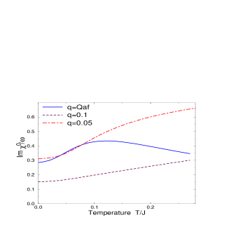
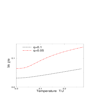
FIG. 20.: Results of numerical calculations of $\lim_{\omega\rightarrow 0}Im\chi^{0}({\bf Q},\omega)/\omega$ as a function of $T$ for ${\bf q}$ in the vicinity of ${\bf Q}_{AF}$ and in the vicinity of ${\bf q}=0$ (a) and of $\lim_{\omega\rightarrow 0}Im\chi({\bf Q},\omega)/\omega$ for ${\bf q}$ in the vicinity of ${\bf q}=0$ ($t^{\prime}/t=-0.3$, $t/J=1.9$, $Z/t=0.166$) (the existence of SC state is ignored). We can not present the latter function for both cases at the same graph due to the very different scale : it is enhanced very stronly in the case of ${\bf Q}_{AF}$.

Let’s analyze now an $\omega$ dependence of the imaginary part of the spin susceptibility, $Im\chi$, taken around ${\bf q}={\bf Q}_{AF}$ which corresponds to the characteristic measured by neutron scattering.

Results of numerical calculations of $Im\chi({\bf Q}_{AF},\omega)$ as a function of $\omega$ performed based on (32) and (11) for fixed doping and increasing temperature are shown in Fig.21. [To analyze the spin dynamics it is preferable to use the complete form (32), (11), (1) rather than the analytical form (34) valid only for $\omega<\omega_{c}(T)$.]

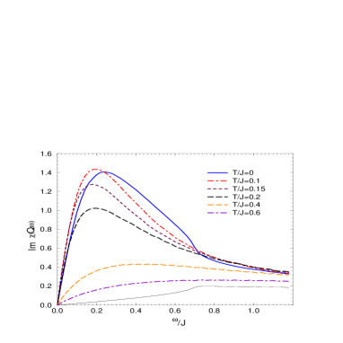
FIG. 21.: Energy dependences of $Im\chi({\bf Q}_{AF},\omega)$ for the underdoped regime for fixed doping and increasing temperature. For a comparison we show also the bare susceptibility $Im\chi^{0}({\bf Q}_{AF},\omega)$ for $T=0$ (the thin line). ($t^{\prime}/t=-0.3$, $t/J=1.83$, $Z/t=0.29$ For chosen doping $T^{*}_{Re}/J\approx 0.1$ and $T^{*}_{Im}/J\approx 0.2$ ($\delta=0.1$)

Due to the small value of $\kappa^{2}_{exc}=1-\alpha$ for $T<T^{*}_{Re}$ there is a strong enhancement at low $\omega$ in comparison with the bare $Im\chi^{0}$. The position of the low energy peak is given by

$$\omega=\omega_{0}=\frac{\kappa^{2}_{exc}}{C}$$ (44)

under the condition $\omega_{0}\ll\omega_{c}$. This condition is necessary in order $C$ to not depend on $\omega$. What is important : the condition $\omega_{0}\ll\omega_{c}$ is fulfilled for all dopings within the rigid SDW liquid state $T<T^{*}_{Re}(\delta)$ due to the specific behaviour of $\kappa^{2}_{exc}$ discussed in subsection IIIb.

We can distinguish three low temperature regimes for $Im\chi$. The first, for $T<T_{F}(\delta)$, is the regime where both $\kappa^{2}_{exc}$ and $C(\omega_{0})\approx C(0)$ do not depend on $T$. $T_{F}$ is very low (see Fig.12) so that this regime can hardly be detectable. The second regime, for $T_{F}(\delta)<T<T^{*}_{Re}(\delta)$, corresponding to the reentrant rigid SDW liquid state is the regime where $\kappa^{2}_{exc}$ slightly decreases with $T$ while $C(\omega_{0})\approx C(0)$ increases with $T$. As a result in this regime the energy of the peak, $\omega_{0}$, decreases with increasing $T$ (reentrant behaviour). The third regime, occuring for $T^{*}_{Re}<T<T^{*}_{Im}$ (i.e. within the zone of quasi phase transition) is the regime in which $\kappa^{2}_{exc}$ starts to increase with $T$ while $C(\omega_{0})$ continues to grow. As a result in this regime the energy of the peak, $\omega_{0}$, is unchanging with increasing $T$.

Both latter behaviours are anomalous. For an usual metal considered in a critical regime above a magnetic phase transition, $\kappa^{2}_{exc}$ decreases with increasing $T$ and $C$ is constant as $T$ increases that leads to the ordinary behaviour with the low energy peak moving towards high energies with increasing $T$. For the system under consideration such a behaviour occurs in the regime, $T>T^{*}_{Im}$, i.e. after passing the zone of quasi phase transition.

The value of $Im\chi$ at the peak position is equal to $4JIm\chi({\bf Q}_{AF},\omega_{0})=1/2\kappa^{2}_{exc}$. It practically does not change with $T$ in the first regime, even slightly increases with increasing $T$. For the second and third regimes, $T>T^{*}_{Re}$, $Im\chi({\bf Q}_{AF},\omega_{0})$ decreases with increasing $T$ in the ordinary way.

Is it possible to observe experimentally the discussed above anomalous regimes ? It is difficult because the low temperature regimes are hidden under the SC phase. Nevetheless it is possible for very underdoped materials. [Another possibility would be a neutron experiment in a pulsed magnetic fields]. Although INS data in the normal state are in general in a good agreement with our results (see for example [32] there is no data available concerning the behaviour of $Im\chi({\bf Q}_{AF},\omega)$ as a function of $\omega$ obtained in progressive changing $T$ for temperature range just above $T_{c}$. For example the recent data for the normal state in highly underdoped YBCO [33] correspond to $60K$ and to $200K$, i.e. there is an important jump in temperature, probably across different regimes. To verify the predicted anomalous behaviour it is desirable to perform such measurements in progressive changing $T$. In fact our proposal is a way to observe $T^{*}(\delta)$ by INS (as it is still one of a few experiments where $T^{*}(\delta)$ has not yet been observed).

IV Summary and discussion

The results obtained in the paper have two aspects : one fundamental and one concerning the high-$T_{c}$ cuprates.

The fundemental aspect is following. We have shown that a 2D system of noninteracting electrons on a square lattice with hoping between more than nearest neighbours undergoes a specific electronic topological transition (ETT) at some electron concentration $\delta=\delta_{c}$. The point of ETT is a $T=0$ quantum critical point with several characteristic aspects. The first aspect is related to the local change of topology of the FS near SP’s. This results in singularities in thermodynamic properties, in a ferromagnetic response function, in an additional divergence of the superconducting response function. From this point of view it is a QCP of a gaussian type. [The logarithmic singularity in a density of states at $\omega=0$ is a consequence of this aspect of ETT not a reason]. The other aspects are related to the topological change at $\delta=\delta_{c}$ in mutual properties of the FS in the vicinities of two different SP’s. As a result, the behaviour of the system is very asymmetrical on two sides of the ETT, the point $\delta=\delta_{c}$ appears as the end of the critical line of static Kohn singularities in the polarizability of noninteracting electrons which exists on one side of QCP, $\delta>\delta_{c}$. On the other side, $\delta<\delta_{c}$, Kohn singularity manifests itself as the line of the dynamic singularities. The dynamic singularities at $T=0$ are transforming into static anomalies at finite temperature. All this happens for the characteristic wavevector for this regime ${\bf q=Q}_{AF}$.

The specific behaviour of the system of noninteracting electrons related to ETT leads to the anomalous behaviour of the system in the presence of interaction. The anomalies exist whatever is a type of interaction : in a triplet or singlet channels, $\bf q$ dependent or $\bf q$ independent, since the motor for them is the ETT in the noninteracting system. We study some of the anomalies. For example we show that the line of instability of the initial metallic state against SDW or CDW order (depending on the type of interaction) has the anomalous form : it grows from the QCP with increasing the distance from QCP instead of having the ordinary form of the bell around QCP. We show that in the metallic state out of this phase there is a characteristic temperature for each electron concentration, $T^{*}_{Re}(\delta)$, which is the temperature of an almost phase transition : a rigidity of the metallic state and the correlation length are maximal at $T=T^{*}_{Re}(\delta)$ when approaching from above and from below. We show that the state below $T=T^{*}_{Re}(\delta)$ (and out of the ordered phase) is characterized by a very specific behaviour. It is almost frozen in distance from QCP and reentrant in temperature rigid SDW (or CDW) liquid. We study some properties of this state. [Some details of the anomalous behaviour depend on interaction. When analysing we have choosen to consider the $\bf q$ dependent interaction in a triplet channel in a view of the following applications to high-$T_{c}$ cuprates.]

All these anomalies happen on one side of QCP, $\delta<\delta_{c}$. On the other side, $\delta>\delta_{c}$, the behaviour is quite ordinary. For example, the correlation length decreases monotonically and quite rapidly with $T$ and with the distance from QCP, $|\delta-\delta_{c}|$, the line of of SDW or CDW ”excitonic” instability behaves in the ordinary way etc.

To finish with the fundamental aspect we would like to emphasize that the considered ETT is quite general and exists in all cases of hoping between more than nearest neighbours: $t^{\prime}\neq 0$ or/and $t^{\prime\prime}\neq 0$ etc. For any set of these parameters one can introduce an effective $\tilde{t}^{\prime}$ and map the situation into the considered in the paper generic model. The exceptions are some sets [20], including $t^{\prime}=t^{\prime\prime}=...=0$, for which the last aspect of the ETT disappears : the QCP is no more the end of the line of static Kohn singularities, the behaviour is absolutely symmetrical on two sides of $\delta=\delta_{c}$. This case corresponds to the nested FS. And although the first aspect of criticality still exists (with the ”famous” Van Hove singularity scenario) all discussed in the paper anomalies disappear. We emphasize this again to avoid a misunderstanding : the considered in the paper scenario has nothing to do with the Van Hove singularity.

The second aspect of the paper is an application of the theory to the hole-doped high-$T_{c}$ cuprates. These materials are quasi-2D systems, the electron FS observed experimentally has such a shape which implies the existence of hoping $t^{\prime}$ (or/and $t^{\prime\prime}$, etc.), the shape of FS changes continuously towards the form corresponding to the ETT when moving from the underdoped side towards the optimal for superconductivity doping. On the other hand, the observed experimentally (by INS and NMR) strong spin dependent response around ${\bf q}={\bf Q}_{AF}$ is a phenomenological argument in a favour of the strong momentum dependent interaction in a triplet channel.

All these features allow us to apply the theory to the high-$T_{c}$ cuprates and to consider the discussed scenario of the anomalous behaviour as a very probable origin of the anomalies observed in the underdoped regime of the hole-doped high-$T_{c}$ cuprates.

In the present paper we have considered some properties and have compared them with experiments. The most important result is of course the existence of the generic temperatures $T^{*}_{Re}(\delta)$ and $T^{*}_{Im}(\delta)$ which give rise to the existence in the metallic state out of the ordered phase of the characteristic temperatures $T^{*}$, different for different properties, but always proportional to $\delta_{c}-\delta$. This is in a good agreement with the general situation in the cuprates. We have considered some concrete examples. We analyse the behaviour of the physical characteristics corresponding to the nuclear spin lattice relaxation rate $1/T_{1}T$ and to the nuclear transverse relaxation rate $1/T_{2G}$ on copper. We have shown that the latter is almost constant as a function of $T$ until some temperature $T=T^{*}_{1/T_{2G}}$ and then decreases with $T$. On the other hand, the first function increases with increasing $T$ until $T^{*}_{1/T_{1}T}$ and then decreases. The characteristic temperatures are different and $T^{*}_{1/T_{1}T}>T^{*}_{1/T_{2G}}$. All these features explain quite well the experimentally observed behaviour, see for example [2]. We show that the behaviour of the spin responce function is quite different in the cases of $\bf q$ around ${\bf Q}_{AF}$ and $\bf q$ around $\bf q=0$ being completely independent. Fluctuations corresponding to small $\bf q$ are also critical in a proximity of the ETT being however not enhanced due to the sign of the interaction. This can explain the observed experimentally qualitatively different behaviout of $1/T_{1}T$ on oxygen and cooper [21]. We have analyzed briefly the behaviour of the characteristics corresponding to that measured by INS and we have demonstrated how $T^{*}$ can be seen in neutron scattering experiment. As to the correlation length there are at present two contradictory conclusions [34, 35] about its behaviour based on the same measurements (performed unfortunetely starting from quite high temperature). Since the method is indirect, an answer depends crucially on the model for the $\bf q$-dependence used to extract $\xi$. In both cases [34, 35] the used models are standard : the lorentzian and the gaussian. As we have seen, the $\bf q$ dependence can be quite nonstandard so that one should be very cautious when interpretating the experiment. As to INS data, they give only a $\bf q$ width of $Im\chi$ at finite $\omega$ not a $\bf q$ width of $Re\chi$ at $\omega=0$ which corresponds to the correlation length. And although the INS data show a $\bf q$ width not depending on $T$ (that indirectly can be considered as an argument in a favour of our theory) it can not be considered as a crucial experiment for $\xi$.

More detailed analysis of NMR and INS will be performed elsewhere. Electronic properties in the ordered SDW ”excitonic” phase and in the reentrant SDW liquid state are considered and compared with ARPES in [10, 11] respectively.

REFERENCES

- [1] H.Alloul,T.Ohno, P.Mendels, Bull.Am.Phys.Soc. 34, 633 (1989); Phys.Rev.Lett. 63, 1700 (1989); W.W.Warren et al, Phys.Rev.Lett. 62, 1193 (1989); G.V.M.Williams et al Phys.Rev.Lett. 78, 721 (1997);
- [2] M. Takigawa, Phys.Rev.B 49, 4158 (1994)
- [3] H.Ding, T. Yokoya, J.C. Campuzano et al, Nature (London), 382, 51 (1996); H.Ding, J.C. Campuzano, M.R. Norman, cond-mat/9712100
- [4] S.L. Cooper et al, Phys.Rev.B 40, 11358 (1989); Puchkov et al, Phys.Rev.Lett. 77, 3212 (1996)
- [5] H.Y.Hwang et al, Phys.Rev.Lett. 72, 2636 (1994)
- [6] J.L.Talon, J.R. Cooper, P.S.I.P.N. de Silva et al, Phys.Rev.Lett. 75, 4114 (1995)
- [7] J.W. Loram et al, Phys.Rev.Lett. 71, 1740 (1993)
- [8] D.C. Johnston, Phys.Rev.Lett. 62, 957 (1989)
- [9] R. Nemetschek et al, Phys.Rev.Lett. 78, 4837 (1997)
- [10] F.Onufrieva, M. Kisselev, P.Pfeuty, to be published
- [11] F.Onufrieva, P.Pfeuty, to be published
- [12] L. Van Hove, Phys.Rev. 9, 1189 (1953). The existence of the logarithmic singularity in the density of states for 2D case was first shown by E. Montroll [13] for the case of phonon density of states.
- [13] E. Montroll, J.Chem.Phys. 15, 575 (1947)
- [14] W.Kohn Phys.Rev.Lett. 2, 393 (1959)
- [15] L.Roth, H.J. Zeiger, T.A. Kaplan, Phys.Rev. 149, 519 (1966)
- [16] T.M. Rice, Phys.Rev.B 2, 3619 (1970)
- [17] More presisely, it exists in all cases or/and etc. except for the special set of the parameters (including the case ) corresponding to the perfect nesting of FS.
- [18] I.M. Lifshitz, Zh. Eskp. Teor. Fiz. 33, 1569 (1960)
- [19] A.A. Varlamov, V.S. Egorov, A. Pantsulaya, Adv. in Phys. 38 , 465 (1989)
- [20] F.Onufrieva, P.Pfeuty, to be published
- [21] R.E. Walstedt, B.S. Shastry, S.W.Cheong, Phys.Rev.Lett. 72, 3610 (1994)
- [22] F.Onufrieva, P.Pfeuty, to be published
- [23] B.I. Halperin, T.M. Rice, Solid State Phys., 21, 115 (1968); A.Kozlov, L.Maximov, Sov.Phys.JETP, 21, 790 (1965)
- [24] Scaling is the main property of a quantum critical point. In Sec.II.C we gave scaling forms for and . The functions and can also be shown to scale with the scaling variable and a very anomalous scaling function. This point will be discussed in another paper.
- [25] F.Onufrieva, S.Petit, Y.Sidis Phys.Rev.B 54, 12464 (1996)
- [26] No true finite ordered state is possible in 2D system in the case of continuous symmetry of the Hamiltonian and only a possible Kosterlitz-Thouless transition is expected. RPA finite transitions should be interpreted for pure 2D system as crossover signaling the appearence of large but finite correlation length. However a weak 3D coupling or small anisotropy of the Hamiltonian are sufficient to induce true LRO.
- [27] The form (34) is close to the phenomenological susceptibility introduced by A.Millis et al [28] if one considers . [This form has been used in many following papers by D.Pines et al (see for example [29]) and A.Chubukov et al (see for example [30])] As we have shown this form is valid only for very low , . For higher , there is an effect of the effective ”pseudogap”. We mean that is no more constant when is not extremely small, see Fig.8. Another important difference is that this form represents only fluctuations in the vicinity of . As we have shown in Sec.II there is also a singularity of in the vicinity of and the fluctuations related to that. Their behaviour is very different from the behaviour of fluctuations in the vicinity of that leads to an independent behaviour of and as functions of and . And finally and most important is that the parameters in the form (34) behave in a very untrivial way as functions of and as discussed in the text.
- [28] A. Millis, H. Monien, D. Pines, Phys.Rev.B 42, 167 (1990)
- [29] V. Barzykin, D.Pines, Phys.Rev.B 52, 13585 (1995)
- [30] A. Chubukov, D. Morr, cond-mat/9701196
- [31] Analysis of the behaviour of the parameter describing a proximity to SC phase is performed in details in [22]; however it is clear from the breaf analysis performed in the Subsec.IIE that it behaves in the ordinary way, i.e. increases quite rapidly when one goes away from the critical line . Therefore, except for an intime vicinity of , it is valid : .
- [32] L.P. Regnault, P. Bourges, P. Burlet et al, Physica C 235-240, 59 (1994)
- [33] P. Bourges, H.F. Fong, L.P. Regnault et al, Phys.Rev.B 56, R11439 (1997)
- [34] J. Bobroff, H. Alloul, Y. Yoshinari, Phys.Rev.Lett. 79, 2117 (1997)
- [35] D. Morr, J. Schmalian, R. Stern, C.P. Slichter, cond-mat/9801317